Calibration, Selection and Identifiability Analysis of a Mathematical Model of the in vitro Erythropoiesis in Normal and Perturbed Contexts
Abstract
The in vivo erythropoiesis, which is the generation of mature red blood cells in the bone marrow of whole organisms, has been described by a variety of mathematical models in the past decades. However, the in vitro erythropoiesis, which produces red blood cells in cultures, has received much less attention from the modelling community. In this paper, we propose the first mathematical model of in vitro erythropoiesis. We start by formulating different models and select the best one at fitting experimental data of in vitro erythropoietic differentiation obtained from chicken erythroid progenitor cells. It is based on a set of linear ODE, describing 3 hypothetical populations of cells at different stages of differentiation. We then compute confidence intervals for all of its parameters estimates, and conclude that our model is fully identifiable. Finally, we use this model to compute the effect of a chemical drug called Rapamycin, which affects all states of differentiation in the culture, and relate these effects to specific parameter variations. We provide the first model for the kinetics of in vitro cellular differentiation which is proven to be identifiable. It will serve as a basis for a model which will better account for the variability which is inherent to the experimental protocol used for the model calibration.
1Introduction
Erythropoiesis is the process by which red blood cells are produced. It occurs within the broader frame of haematopoiesis, the process which generates all blood cells. The dynamics of haematopoiesis has been extensively modelled mathematically in the past decades, with the first historical models published as early as fifty years ago [1, 2] (for a review of the history of haematopoiesis modelling in general, see [3]). Models of haematopoiesis have improved the understanding of both the processes they describe [4], and the mathematical tools they use. These models comprise non-exhaustively Differential Equations (DE, either ordinary [1, 2, 5], partial, which can be structured by age, maturity, or a combination of these [6], or even delay differential equations [7]) and agent-based models [8]. They can be fully deterministic [5] or can include a more or less prominent stochastic component [9– 11].
Recent works specifically focusing on erythropoiesis comprise DE-based models [12, 13] and multi-scale descriptions of these phenomena [14– 16].
All these works aim at modeling the in vivo physiological processes, i.e. the processes occurring in a whole organism. Those processes are related to numerous pathologies, for which clinical data are very sparse and must be acquired on experimentally prohibitive time-scales, which complicates their study. Modeling has therefore provided significant insights into these pathologies [4]. On the contrary, the in vitro context, i.e. the process that takes place in cells grown in culture, is much simpler to characterize experimentally. Yet, to our knowledge, no modeling study has focused on it so far. Since the in vitro differentiation is an experimental tool of choice for the study of cellular decision-making [17– 19], we propose to develop a model for the dynamics of the in vitro erythropoiesis.
Moreover, the current models of erythropoiesis suffer from one major drawback: the weakness of their parameterization, which can fall within three categories.
A vast majority of the existing models of erythropoiesis are based on experimental parameter values from the literature. In some cases these values are used in other contexts that those in which they were obtained (typically, in other species [12]).
In other cases, the parameter values of a model are chosen arbitrarily to reproduce a qualitative behaviour. Apart from this qualitative fit, such approaches do not provide any information regarding the validity of the values [16].
Finally, when the parameters of a model are estimated to reproduce a dataset, the precision of this estimation is seldom investigated [20]. By this, we mean that depending on the algorithmic details of the estimation, it is possible that several values of the parameters might render the same fit to the data. In this case the model is said to be unidentifiable.
A model is said to be identifiable if and only if it is possible to infer a unique value for each of its parameter by comparing its output to experimental data. Otherwise it is unidentifiable. A model can be non-identifiable for several reasons [21, 22].
Structural identifiability is related to the structure of the model, and the observed variables. A model is structurally unidentifiable when several of its parameters are redundant, meaning that they can vary in such a manner that the measured output of the model is not affected [21– 23]. A variety of methods, based on different approaches, can be used to assess the structural identifiability of a dynamic model. These include, non-exhaustively, the Taylor series method [24], the similarity transformation [25], the generating series method [26], and the profile likelihood approach [22, 27, 28]. A review of these methods is provided in [21] and their performance is assessed in [23].
Practical Identifiability is related to the quantity and quality of the data used for model calibration. If the data is too sparse or too noisy to estimate all parameters together, then the model is said to be practically unidentifiable [21, 22]. Essentially three kinds of frequentist methods can be used to assess the practical identifiability of a model: methods based on the Fisher Information Matrix (FIM) [29], which use a parabolic approximation of the likelihood function, profile-likelihood-based methods [22, 28], and bootstrapping, which is based on the resampling of the data [30]. FIM-based methods are less computationally demanding, because they require the fewest parameter estimation steps [31], but due to their parabolic approximation they are proven to render biased results [22]. On the other hand, the profile likelihood-based method is computationally cheaper than bootstrapping [31], and is proven to detect both structural and practical unidentifiabilities [22, 27].
Despite the growth of the interest in identifiability and related concepts among the biological systems modelling community [21, 32– 34] the identifiability of models remains seldom investigated [20]. With this in mind, the most rigorous way to design and calibrate a model of erythropoiesis seems to use dedicated experiments to determine its parameter values. Once these values have been determined, one should then test the identifiability of the model before using it for any prediction.
In this paper, we aim at developing an identifiable model for the dynamics of the in vitro erythroid differentiation. The data that we generated to calibrate it consists in counts of different cell sub-populations at regularly spaced time-points during the course of proliferation and differentiation of chicken erythroid progenitors. We start by formulating different possible structures for the dynamics of the system, and for the distribution of residuals. We select the best structure and distribution using classical information criteria. We then assess the identifiability of our model using an approach based on the profile likelihood concept. Finally, we test the adaptation of our model in a perturbed context, when cells are exposed to rapamycin, a drug which is known to affect the dynamics of differentiation, although its precise effect on proliferation and differentiation remains unclear. Since our model is identifiable, it is possible to quantify the effect of the drug on each of its parameters.
2Methods
2.1Experimental Data
2.1.1T2EC cell culture
The experimental setting from which all the data used in this study were obtained consists in a culture of chicken erythroid progenitors called T2EC that were extracted from the bone marrow of 19 days-old SPAFAS white leghorn chickens embryos (INRA, Tours, France). They may either be maintained in a proliferative state or induced to differentiate into mature erythrocytes depending on the medium in which they are grown [35].
2.1.2LM1 experiment
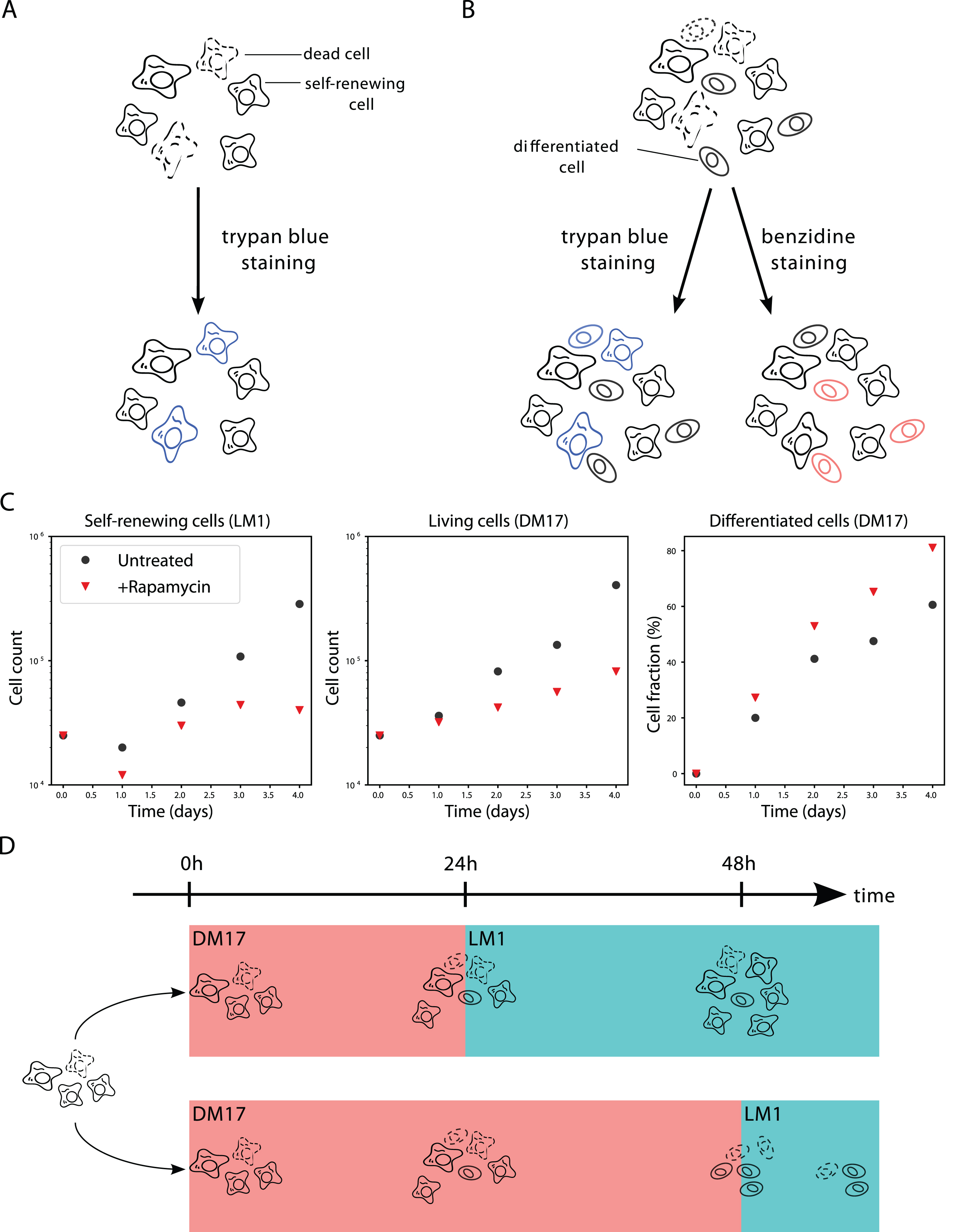
In the self-renewal medium (referred to as the LM1 medium) the progenitors self-renew, and undergo successive rounds of division. LM1 medium was composed of α-MEM medium supplemented with 10% Foetal bovine serum (FBS), 1 mM HEPES, 100 nM β-mercaptoethanol, 100 U/mL penicillin and streptomycin, 5 ng/mL TGF-α, 1 ng/mL TGF-β and 1 mM dexamethasone as previously described [35]. After 10 days in LM1, the culture is composed at >99% of erythroid progenitors cells [36, 37]. Cell population growth was evaluated by counting living cells in a 30 μL sample of the 1mL culture using a Malassez cell and Trypan blue staining (SIGMA), which specifically dyes dead cells (Fig. 1-A), each 24h after the beginning of the experiment.
Fig.1
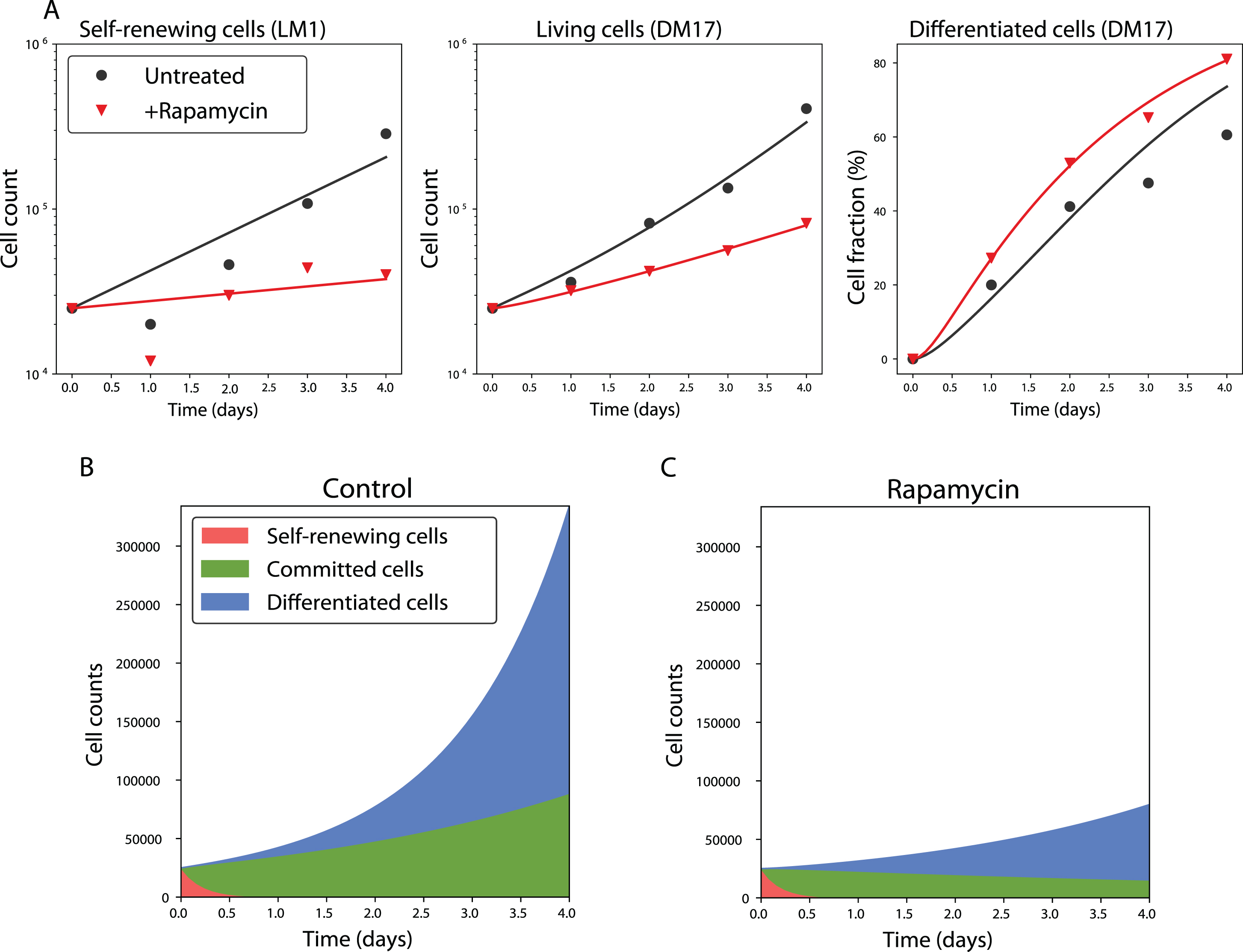
Experimental context. A: In LM1 medium the culture is only composed of living and dead cells in the self-renewal state. The amount of living cells can be measured by trypan blue staining. B: In DM17 medium, the culture is a mixture of living and dead, self-renewing and differentiating cells. The amount of living cells can be measured by trypan blue staining. The amount of differentiated cells can be measured by benzidine staining. C: Data used to calibrate the models. Black dots are the results of a single experiment in the control situation (no treatment). Red triangles are the results of the same experiment under rapamycin treatment. Both conditions were obtained with the same initial populations, so the black dot and red triangle are the same at t = 0. For readability, living cell counts are displayed in log-scale, and differentiated cell counts are displayed as a fraction of the total living cell count. D: Commitment experiment. If the differentiating cells are switched back to LM1 after 24h of differentiation the culture starts proliferating again (upper trajectory). If the cells are switched back to LM1 after 48h, the culture stagnates (lower trajectory).
2.1.3DM17 experiment
T2EC can be induced to differentiate by removing the LM1 medium and placing cells into 1mL of the differentiation medium, referred to as DM17 (α-MEM, 10% foetal bovine serum (FBS), 1 mM HEPES, 100 nM β-mercaptoethanol, 100 U/mL penicillin and streptomycin, 10 ng/mL insulin and 5% anaemic chicken serum (ACS)). Upon the switching of culture medium, a fraction of the progenitors undergoes differentiation and becomes erythrocytes. The culture thus becomes a mixture of differentiated and undifferentiated cells, with some keeping proliferating. Cell population differentiation was evaluated by counting differentiated cells in a 30 μL sample of the culture using a counting cell and benzidine (SIGMA) staining which stains haemoglobin in blue (Figure 1B). A parallel staining with trypan blue still gives access to the overall numbers of living cells (Figure 1B). Consequently, the data available from this experiment are the absolute numbers of differentiated cells, as well as the total number of living cells (which comprises both self-renewing and differentiated cells) at the same time points as in the LM1 experiment. The data presented on Figs 1C and 5A are the total number of living cells in the culture, and the fraction of differentiated cells, extrapolated from the counting.
2.1.4Rapamycin treatment
In the control condition, cells were grown in their regular medium with 0.1% DMSO (Figure 1C, black dots). In the treated condition, cells were grown in the presence of rapamycin (Calbiochem), a chemical drug known to affect both the number of living cells in culture, and the proportion of differentiated cells [36, 38], as displayed on Figure 1C. Cells were treated with Rapamycin at 50 nM just after switching them to the DM17 medium. It should be noticed that the very same original culture was used to initiate all the experiments presented on Figure 1C (in the LM1 and DM17 media, as well as in the treated and untreated conditions).
2.1.5Commitment experiment
Another piece of experimental data that will be of use for calibrating our models is the result of the commitment experiment. The full protocols and results of this experiment are described in Figure 10 of [17] and are summarized on Figure 1D. In this experiment, once a cell culture has been switched to the DM17 medium, it can be switched back to the LM1 medium. Switching back after 24 hours of differentiation does not cancel the self-renewing ability of the progenitors, but switching back after 48 hours does: instead of proliferating again, the culture stagnates. This means that there must remain some self-renewing cells in the culture after one day, but that they all have started differentiating after two days.
2.2Models
2.2.1Structural Model
We propose three alternative dynamic models of the erythroid differentiation, which are summarized on Figure 2.
Fig.2
Diagrams of three possible dynamic models for our data. A: The SB model has no intermediary compartment. B: The S2B model has no intermediary compartment, but the self-renewing cells change proliferation rate in DM17. C: The SCB model has an intermediary compartment.
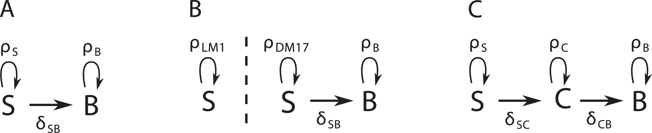
The SB model comprises only two compartments (Figure 2A), a self-renewing one (S) and a differentiated one (B, which stands for benzidine-positive), whose dynamics are given by the equations:
This model is characterized by a set θ = (ρS, δSB, ρB) of three parameters, where ρi is the net proliferation rate of compartment i. For estimation-related reasons, it incorporates the balance between cell proliferation and cell death. This means that ρi can be either positive (more proliferation than death) or negative (more death than proliferation). On the other hand δij is the differentiation rate of cell type i into cell type j, which is positive.
The S2B model comprises also the S and B compartments (Figure 2B), but allows the self-renewing cells to change their net proliferation rate upon culture medium switching. This formulation arose from the consideration that proliferation is faster in the DM17 than in the LM1 medium (Figure 1C). The dynamics of this model are given by the equations:
It is characterized by the set (ρLM1, ρDM17, δSB, ρB) of four parameters, following the same notation convention as in the SB model.
Finally, the SCB model (Figure 2C) also comprises the same self-renewing and differentiated compartments as the SB model, as well as a hypothetical committed cells compartment C. This compartment comprises intermediary cells that are committed to differentiation, yet not fully differentiated. The dynamics of these three compartments are given by the equations:
It is characterized by the set (ρS, δSC, ρC, δCB, ρB) of five parameters, following the same naming convention as the two other models.
Moreover, it should be noted that differential systems (1) to (3) are fully linear, and that their matrices are lower-triangular, which makes them easily solvable analytically. Their simulation is thus very fast. The detail of the analytical solutions to these systems is given as supplementary material.
Finally, not all variables in the models can be measured through the experiments that we presented in section 2.1, and we only have access to two observables of the system: the total amount of living cells T (t) through trypan blue staining, and the amount of differentiated cells B through benzidine staining. The number of living cells T can be measured in LM1 and in DM17, yet in LM1 there is no differentiation, so in the LM1 experiment T = S (or T = SLM1 in the S2B model). The number of differentiated cells B can be measured in DM17 (it is null in LM1).
2.2.2Error Model
In order to properly define the likelihood of our model, we need to define a statistical model for the prediction error of our dynamical model, y - f (t, y0, θ), where y is the data and f the prediction from the dynamical model (which depends on time t, the initial condition y0 and the parameters θ of the model). This prediction error is usually modelled by a gaussian distribution with a null mean [22, 39, 40]. Then, the standard deviation of the error remains to be characterized.
When dealing with small datasets, a reasonable option is to build an additional model layer for the standard deviation of the error [39]. This means finding a suitable function g, of the time t, the initial condition y0, the dynamical parameters θ and possibly other parameters ξ (which we will call the error parameters), to describe this variance. The error model is then completely described as:
With this representation, the log-likelihood of the model follows as:
(4)
where n is the number of variables of the dynamic model, and m the number of measurement points for each variable, and from which the log (2π) term is dropped. In the end, the best-fit parameters of the model are the values of θ and ξ which minimize the quantity defined in Equation (4). In this equation, the data yi,j and the prediction fi (tj, θ) are the total number of cells in each measured compartment of the model (without any transformation of the variables).
2.3Parameter Estimation
Considering the data at our disposal, we adopted the following procedure for parameter estimation:
1. Estimate ρS (or ρLM1 in the S2B model), and the corresponding error parameters ξ1 from the LM1 experiment. In LM1 there is no differentiation, so the S compartment just follows an exponential growth with rate ρS.
2.
(a) In the SB model, set δSB so that there are no more self-renewing cells after 2 days of differentiation (which we interpret as S (48h) ≤1, i.e.
(b) In the SCB model, set δSC so that there are no more self-renewing cells after 2 days of differentiation (which we interpret as S (48h) ≤1, i.e.
3. Estimate the remaining parameters, and the corresponding error parameters ξ2, using the data from the DM17 experiment. In the SB model, the only remaining parameter is ρB. In the S2B model, the remaining parameters are ρDM17, δSB and ρB. In the SCB model, these are ρC, δCB, ρB.
The second step of this estimation sets δSC (δSB in the SB model) to a value such that there are no more self-renewing cells after 2 days of differentiation. This observation does not come from the cellular kinetics experiment that we presented on Figure 1C. It rather uses the results of the commitment experiment (Section 2.1.5 & Figure 1D), which shows that some self-renewing cells remain in the culture after one day, but that they all are differentiated after two days [17].
In the SCB model, considering that the self-renewing compartment S is characterized by an exponential dynamic, and that there are no more self-renewing cells if and only if S ≤ 1, this provides an upper and a lower bound for δSC:
(5)
For the sake of simplicity, we will set
These considerations do not affect the S2B model, in which the switching of the culture medium only affects the proliferation rate of the S compartment.
In both estimation steps, the -log likelihood was minimized using the Truncated Newton’s algorithm [41, 42] implemented in the python package for scientific computing scipy [43]. Convergence to the global minimum was assured by a random sampling of the initial guesses for parameter values (Figure S1).
2.4Model Selection
In order to choose a proper error model, one needs to adopt a selection criterion, which allows to rank models and keep only the best ones, by balancing the quality of the fit of the models with their complexity.
We used a selection approach based on the corrected Akaike’s Information Criterion (AICc, [44]):
(6)
where k is the number of parameters of the model and n is the sample size. The corrective term in AICc has been developed for linear models and small samples. However, since there is no selection criterion derived from AIC for non-linear models, the literature recommends using AICc when in doubt [44].
From the AICc values of a set of models, we compute the corresponding Akaike’s weights [44]:
(7)
where wi is the Akaike’s weight of the i-th model, and R is the number of competing models. The Akaike’s weight of a given model in a given set of models can be seen as the probability that it is the best one among the set [44]. In this setting, selecting the best models of a set of models means computing their Akaike’s weights, sorting them, and keeping only the models whose weights add up to a significance probability (for example, 95%).
2.5Identifiability Analysis
We assessed the identifiability of our model using the method based on the statistical notion of profile likelihood [22, 45].
For a model with k parameters, a parameter space
(8)
Namely, the profile likelihood with respect to a parameter at a certain value is the likelihood of the model, maximized with respect to all the other parameters. Computing the profile likelihood at a certain value x of a parameter θi means to set θi = x and to estimate the values of the other parameters θj that minimize the error -2 log (L) in this setting. Consequently, -2 log (PL) is minimal at the optimal parameter values set, and increases in both directions.
It is possible to define a confidence interval CIθi at a level of confidence α ∈]0, 1 [ for a parameter θi, derived from the evaluation of the profile likelihood [22]:
(9)
where
Namely, all the parameter sets that render a profile likelihood closer to its minimal value than a threshold χ2 (α, k) belong to the confidence interval.
A model is then practically identifiable at the level of confidence α if and only if the confidence intervals at level α of all of its parameters are bounded [22]. In this study, we used α = 0.95.
The profile likelihood approach is a good way of addressing the identifiability of a model, because it allows to detect both structural and practical unidentifiabilities. This feature makes the approach more efficient in practice than most of the other methods in the field [21, 23, 27, 46].
3Results & discussion
3.1Measurement error
The data that we used for the calibration of our models are displayed on Figure 1C. For readability, it displays the total cell counts in log scale, and the differentiated cell counts as a fraction of the total count. This representation emphasises the fact that the measured cell population in LM1 decreases between 0h and 24h, in both conditions (control, and rapamycin-treated).
Every time-point displayed on figure 1C was obtained by a single measurement, which increases the measurement error compared to a replicated experiment. We conclude that the observed decrease in the total living cell number in the LM1 medium (in both conditions) is due to the experimental error that the protocol suffers rather than to a hypothetical biological feature of the cells under study.
3.2Fitting the model with no treatment: Model design and validation
3.2.1Choosing a structural and an error model: selection approach
By combining the three error models presented in Table 1 with the three dynamic models presented in Figure 2, it is possible to define 9 different models of our system. In order to choose the best one at reproducing the in vitro dynamics of erythropoiesis, we computed the maximum-likelihood estimates of the parameters of these nine models, (which are displayed in Table S1).
Table 1
Definition of three different error models [40]
| Error model | Definition of g | Error parameters |
| Constant error | ∀ j gi (tj) = a | ξ = (a) |
| Proportional error | ∀ j gi (tj, y0, θ) = b . fi (tj, y0, θ) | ξ = (b) |
| Combined error | ∀ j gi (tj, y0, θ) = a + b . fi (tj, y0, θ) | ξ = (a, b) |
For each of these nine models, we computed the likelihood-based selection criteria that are displayed on Table 2. The S2B and SCB dynamic models with a proportional error appear as the best ones and offer very similar fits. All other models are far worse (their Akaike’s weights add up to around 4 × 10⁻⁴) but it remains impossible, based on this criterion, to decipher which of the two remaining models should be used to best describe the in vitro erythropoiesis.
Table 2
Selection criteria evaluated for the nine possible pairs of error model and dynamic model
| Dynamic model | Error model | -2logL1 | -2logL2 | k | AIC | AICc | ΔAICc | wAICc |
| SB | constant | 107 | 228 | 4 | 343 | 347 | 45 | 8.9 × 10⁻¹¹ |
| SB | proportional | 106 | 199 | 4 | 313 | 317 | 15 | 2.5 × 10⁻⁴ |
| SB | combined | 106 | 199 | 6 | 317 | 328 | 26 | 1.3 × 10⁻⁶ |
| S2B | constant | 107 | 195 | 6 | 314 | 324 | 22 | 7.6 × 10⁻⁶ |
| S2B | proportional | 106 | 174 | 6 | 291 | 302 | 0 | 0.55 |
| S2B | combined | 106 | 174 | 8 | 295 | 319 | 18 | 8.7 × 10⁻⁵ |
| SCB | constant | 107 | 195 | 6 | 314 | 325 | 23 | 6.7 × 10⁻⁶ |
| SCB | proportional | 106 | 174 | 6 | 292 | 302 | 0.40 | 0.45 |
| SCB | combined | 106 | 174 | 8 | 296 | 320 | 18 | 7.1 × 10⁻⁵ |
L1 is the log-likelihood of the model for the LM1 data. L2 is the log-likelihood of the model for the DM17 data. k is the number of estimated parameters in each of the models, according to the procedure described in section 2.3. For each model, the sample size is n = 15. AIC = -2 log L1 - 2 log L2 + 2k is the Akaike’s Information Criterion [44]. AICc is the corrected AIC (Equation (6)). ΔAICc = AICc - min(AICc) is the AICc difference. wAICc is the Akaike’s weight (Equation (7)).
However, the S2B model does not describe the results of the commitment experiment (Figure 1D). In this model indeed, self-renewing cells switch between different self-renewing rates upon medium switching. As a consequence, switching the cells back and forth between the two media should just switch their proliferation rate, without affecting their proliferation ability. So the cells would never lose their proliferation ability, as opposed to the result of the commitment experiment.
On the other hand, the SCB model predicts that upon switching to the differentiation medium, the cells from the S compartment start differentiating. Once they are all differentiated, cells from the C and B compartments can still proliferate, but this proliferation might be cancelled by a switch back to the LM1 medium. It is thus impossible to describe the process of commitment with the S2B model, while it is possible with the SCB model.
As a conclusion, the SCB model with a proportional error is the best-fitting model which also accounts for the results of the commitment experiment, making it our dynamic model of choice for the rest of this study.
3.2.2Identifiability analysis
In order to use a model for predictive purposes, one needs to assess its identifiability. The profile likelihood curves of all estimated parameters are displayed on Figure 3, for the SCB model with proportional error. For ρS and b1, which are estimated together, the identifiability threshold at confidence α = 0.95 is χ2 (0.95, 2) =5.99. For ρC, δCB, ρB and b2, which are also estimated together, the threshold is χ2 (0.95, 4) =9.49.
Fig.3
The SCB model with proportional error is fully identifiable. Solid curves are the profile likelihood curves of each estimated parameter of the model. Dashed lines give the identifiability threshold of each parameter at confidence level α = 0.95.
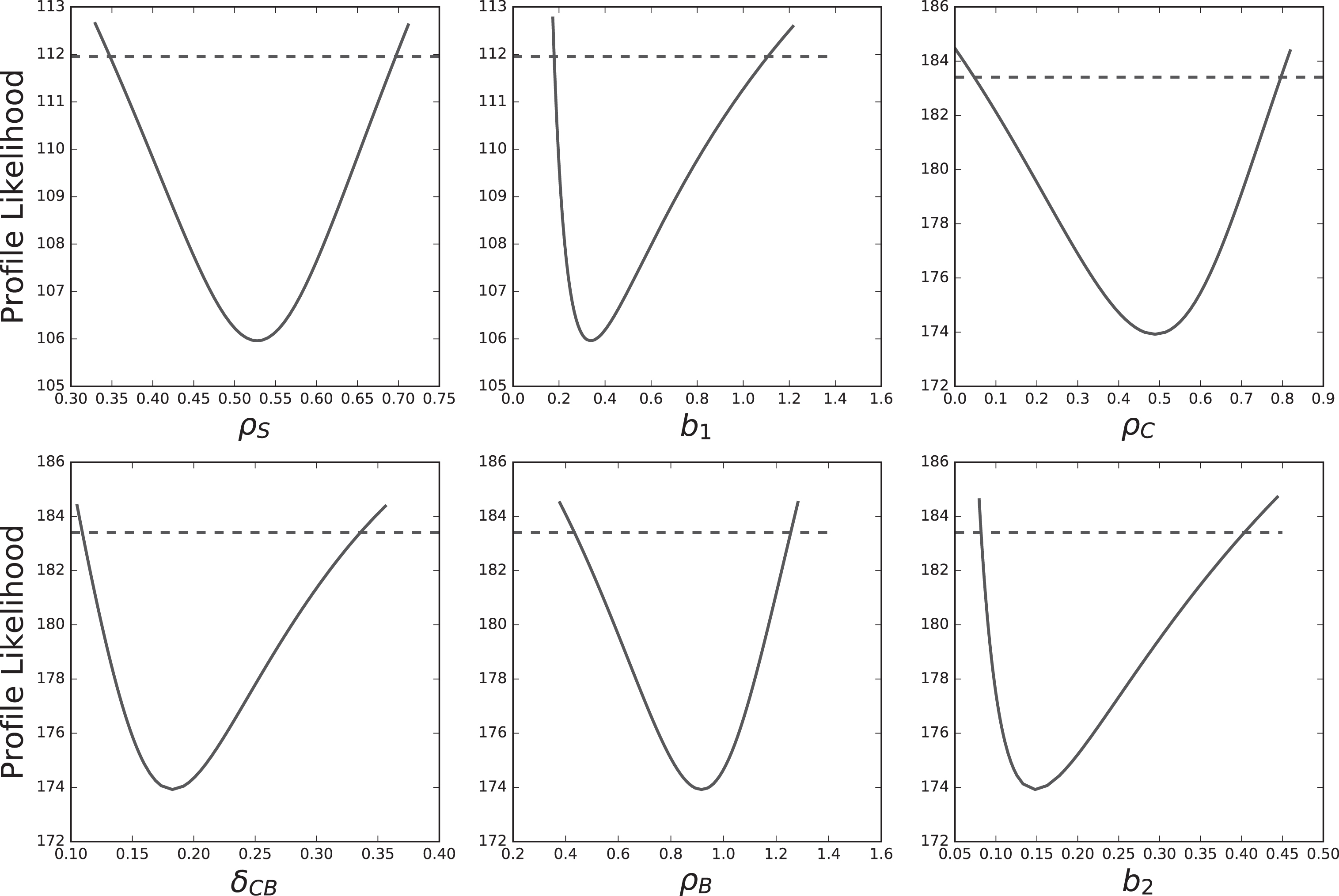
For every parameter of the model, the profile likelihood curve crosses the threshold on both sides of the optimum, which means that every parameter of the model is identifiable, at the level of confidence α = 0.95. The confidence intervals of the parameters [22], extracted from these profiles (Equation (9)) are displayed in Table 3.
Table 3
Confidence Intervals of the parameters of the SCB model with proportional error.
| Parameter | Lower bound | Optimal value | Upper bound |
| ρS | 0.35 | 0.53 | 0.70 |
| (doubling time) | 24 | 31 | 48 |
| b1 | 0.18 | 0.34 | 1.1 |
| δSC | 5.6 | - | 11 |
| (half-life) | 2 | - | 3 |
| ρC | 0.049 | 0.49 | 0.80 |
| (doubling time) | 21 | 31 | 340 |
| δCB | 0.11 | 0.18 | 0.34 |
| (half-life) | 49 | 92 | 150 |
| ρB | 0.44 | 0.92 | 1.3 |
| (doubling-time) | 13 | 18 | 38 |
| b2 | 0.081 | 0.15 | 0.41 |
Highlighted in gray are the confidence interval boundaries at level α = 0.95, extracted from Fig. 3, and the best-fit estimate of all the parameters of the model (expressed in d-1). For δSC, which is not estimated, no optimal value can be computed, but absolute bounds on its values can be computed with Equation (5). Parameters are grouped by their estimation step in our procedure: ρS and b1 are estimated together in the first step, then δSC is set, and finally the four other parameters are estimated together. For the proliferation rates ρS, ρC and ρB, we also give the corresponding doubling times of the populations in hours (i.e. how long would it take to double the population in the absence of differentiation?). For the differentiation rates δSC and δCB, we also give the half-life of the corresponding populations in hours (i.e. how long would it take to differentiate half the cells from the undifferentiated population, in the absence of proliferation?)
For a given parameter, the size of the confidence interval depends on the number of parameters that are estimated together, the required level of confidence, and the likelihood function used for the computation. By definition (Equation (8)), the profile likelihood renders as large of a confidence interval as possible, because it increases as slowly as possible on each side of the optimal parameter value. This means that identifiability is harder to satisfy with the profile likelihood approach than with other definitions, for example based on a linearization of the likelihood surface at the optimal parameter set [22].
As a consequence, the fact that the parameter confidence intervals presented in Table 3 may appear as quite large is not a sign that the parameters are poorly estimated. It is rather the evidence that they remain identifiable even with a very stringent definition of identifiability, and at a high level of confidence.
It is not possible to study the identifiability of δSC, since it is not estimated from the data. However, the commitment experiment (Figure 1D) give us access to a lower and an upper bounds for its value (Equation (5)). We determined the optimal likelihood of the model, and its optimal parameters in this range of value (figures S1 and S2), showing that the choice of δSC does not influence the dynamics of our model.
3.3Modelling differentiation in the control case
A simulation of the model with the identified values of its parameters is reproduced, with the corresponding experimental data, on Figure 5A. The overall quality of the fit is good, especially for the DM17 populations.
The precise values of each parameter of the model are reported in Table 3. The proliferation rate of the committed cells is slightly lower than the one of the self-renewing cells (the net doubling-time of the committed compartment is about 34h, whereas the doubling-time of the self-renewing compartment is around 31h). The differentiated cells proliferate with a higher rate (their doubling time is about 18h). Taken together, these doubling times explain the faster proliferation of cells in the DM17 medium than in the LM1, in agreement with previous data [35]. Finally, the self-renewing cell differentiation is very fast: the lowest possible value of δSC gives them a half-life of 3h in DM17. This means that half of the S compartment would differentiate every 3h in the absence of proliferation. On the contrary, the differentiation of the committed cells is much slower (if they stopped proliferating, they would have a half-life of 90h).
The timescales at which these processes occur are pictured on Figure 5B, which displays the number of cells in each state during a simulation of the model. As specified by the setting of the value of δSC, the population of self-renewing cells quickly collapses, and the culture becomes a mixture of committed and differentiated cells. Both of these compartments then grow at their own rate.
At this stage, we have developed a very simple model of erythroid differentiation, that accounts well for the data used to calibrate it. Plus, it is fully identifiable (at confidence level 95%). We thus use it to study the effect of rapamycin, a drug known to affect the in vitro erythroid differentiation [36, 38].
3.4Modelling differentiation under Rapamycin treatment
Rapamycin is known to increase the proportion of differentiated cells in cultures of chicken erythroid progenitors [36, 38] (Figure 1C). Yet this effect might have several origins: a decreased mortality of the differentiated cells, or an increased differentiation rate for example. To decipher between these different possible effects of the rapamycin treatment, we estimated the values of the parameters of our model in the rapamycin treated case.
To avoid an overparameterization of the rapamycin effect, we considered that for each estimated parameter of the model, the value under rapamycin treatment could be either equal to the value in the untreated case, or equal to another value yet to be estimated. The first option would not introduce a new parameter in the model, but the latter would. Our model has seven parameters (5 dynamical parameters and 2 error parameters), of which 6 only are estimated (since δSC is entirely determined by the value of ρS). This means that we can define 26 = 64 models of rapamycin treatment, by keeping some of the parameters unchanged compared to the untreated case, and re-estimating the others with the data presented on Figure 1C.
Fig.4
Modelling erythropoiesis under rapamycin treatment. A. Akaike’s weights of the three best models of the rapamycin treatment. The 61 other models are not displayed for readability. B. Parameter values in the best model of rapamycin treatment. Red dots are the ratio of the parameter values under rapamycin treatment with their values in the untreated case. Black straight lines represent the confidence intervals of the values in the untreated case, computed from Figure 3. Red straight lines represent the confidence intervals at α = 95% of the values in the treated case, computed with the Profile Likelihood as well (Figure S4). The dashed line indicates the parameter values in the untreated case, by which all parameters are scaled for readability.
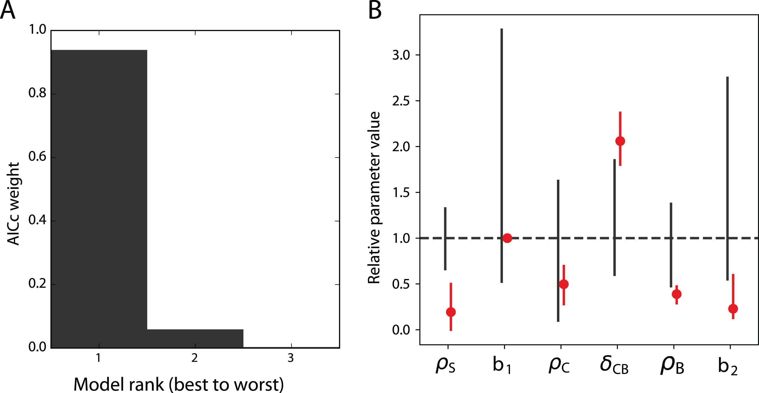
Fig.5
The model reproduces the cellular kinetics observed in vitro. A: Simulation of the SCB model with proportional error in the untreated (black) and rapamycin-treated cases (red). Solid lines represent a simulation of the SCB model with proportional error, with its best-fit parameters. Dots are the experimental data in the untreated condition. Triangles are the experimental data under rapamycin treatment. Displayed are the total number of living cells in LM1 and DM17 media (in log-scale), and the fraction of differentiated cells in DM17, although the fit was performed on the raw cell numbers. B-C: Numbers of cells in each compartment as a function of time in the untreated (B) and treated (C) cases.
We thus estimated the parameters of these 64 possible models of the treatment, and computed their likelihood-based selection criteria, the same way as we did for the dynamic model and the error model (see section 3.2). The Akaike’s weights of the best three of these models are shown on Figure 4A. The best model of the treatment is responsible for 94 % of the weight of the 64 models, making it by far the best model for the rapamycin treatment. A simulation of this model is displayed on Figure 5, which indeed shows the quality of its fit to the data obtained under rapamycin treatment.
This model is obtained by varying all the parameter values except b1, compared to the control case, as displayed on Figure 4B. Moreover, we computed confidence intervals for the parameters that vary under the treatment, showing that all these parameters are identifiable at α = 0.95 (Figure S4). The confidence intervals of ρS, δCB, ρB and b2 show very little overlap with their confidence intervals in the control case, showing the strength of the treatment effects. The three proliferation rates ρS, ρC and ρB are reduced under the treatment, while the differentiation rate δCB is increased.
Finally, the effect of rapamycin on the distribution of cells between the different compartments is displayed on Figure 5C. Under rapamycin, the C compartment decays, when it proliferated in the control case. Moreover the B compartment has a longer doubling time under rapamycin treatment (48h instead of 18h in the untreated case). These two effects explain why the drug treatment reduces the overall amount of cells and increases the proportion of differentiated cells in the culture.
4Conclusion
We proposed a model for the in vitro erythroid differentiation, which comprises two components. First, the dynamic component is the set of ODE written in Equation (3), which describes the dynamics of three cell populations. Second, we added an error component which describes the distribution of the residuals of the dynamic model.
The three populations of our dynamical model are related to three different stages of differentiation of the progenitors. The first one is in a self-renewal state S where differentiation has not started, and the third one has finished differentiating. The second population lies in the middle, in a state of commitment C where cells are not fully differentiated yet, but cannot go back to self-renewal.
Similar 3-states models have already been used to describe differentiation [19]. Their success probably stems from the fact that it would be difficult to describe differentiation as the transition between only 2 states, as we highlighted in the context of in vitro erythropoiesis with our SB model. Actually, differentiation from one cell type to another is a continuous process, so its best description would probably be a continuum of states, which would punctuate the transition between the two cell types [19, 47].
However, explicitly accounting for this continuum would require an infinity of intermediary states. For example, the levels of differentiation factors inside the cell could be used as a measure of its differentiation state [48, 49]. Such kind of a model should be able to describe differentiation more faithfully than ours. Yet our model, though simplistic, reproduces our experimental data quite well, and is identifiable. Moreover, since it is fully linear and thus analytically integrable, its simulation and calibration are very quick.
Such simplicity and identifiability of our model would probably make it valuable to describe differentiation in other contexts.
Once the model was chosen, we verified the accuracy of its parameter estimates. We showed that among the seven parameters of our model, the six that are estimated by the maximum-likelihood approach are identifiable, and that the choice of the seventh one does not alter the behaviour of the others. Using the Profile Likelihood approach, we computed confidence intervals for our parameters. Even though their relatively large size might be interpreted as a lack of accuracy in the estimates of the parameters, it is not the case since the identifiability of a parameter is harder to satisfy by the Profile-Likelihood approach than using other methods. We thus showed that our model is fully identifiable, even using a very stringent criterion.
After demonstrating the validity of our model in the control case, we used it to study the effect of rapamycin, a chemical drug which is known to impact the differentiation of erythroid progenitors [36, 38]. We designed 64 different models of the rapamycin treatment, which differ by the combinations of parameters that are affected by the treatment. Evaluating the quality of their fit to the data allowed us to retain only the best model of rapamycin treatment. The parameter values in this model reveal that rapamycin increases the differentiation rate of the intermediary cell compartment, and reduces the net growth rates of the three other compartments. This means that rapamycin increases the differentiation of the cells in culture, and also affects the balance between their proliferation and mortality. The reduced net proliferation rates might be caused by a reduced proliferation, an increased mortality or any joint variation of the two processes equivalent to one of these effects (e.g. reduced mortality, and an even more reduced proliferation).
In the context of other perturbations of differentiation (for instance, treating cultures with a different drug than rapamycin), should the drug influence be less strong, we might need a more subtle means of parameter evaluation, such as the fused lasso penalized regression [50].
At the moment, our approach suffers one major drawback that is the size of our dataset. Indeed, the precision of our prediction of cell numbers at one time-point relies on the precision of our measures of these numbers. And this measurement precision is directly related to the number of repetitions of the measurements.
Repeating the same experiment several times would thus increase measurement precision and average out measurement noise. This would allow a more precise estimation of the error model parameters, and in turn would increase the precision of the dynamic model. What we call repeating the same experiment here does not simply consist in counting cells from the same time point several times to average out sampling biases. It rather involves putting new cells in culture and following their populations over time, as two full replicates of the experiment.
In this setting, the measurement error would not just be limited to technical noise due to the sampling of cells from the culture for counting. It would rather be related to differences between the kinetic features of the cells in culture, i.e. to actual biological heterogeneity. This heterogeneity would be averaged by the estimation of one parameter set to fit all the data.
One way of accounting for this heterogeneity in a model, without averaging it out during parameter estimation, is through the use of a mixed effect model, that is a mathematical model (e.g. a set of deterministic ODE, like ours) whose parameters are modeled by distributions of random variables [40]. We are presently assessing the ability of such mixed effect models to characterize both the behaviour of the cells in culture on average, as well as their variability.
Authors contributions
AG generated the experimental data used in this study. FC, RD and OG designed the alternative models of differentiation. RD estimated their parameter values, carried out all the subsequent analyses of identifiability and of the effect of rapamycin, and was a major contributor to the manuscript. All authors read and approved the final manuscript.
Supplementary material
[1] The supplementary material is available in the electronic version of this article: http://dx.doi.org/10.3233/ISB-190471.
Acknowledgments
We thank La Ligue Nationale Contre le Cancer (Comité de la Loire) for funding.
The original design of the progenitor cell in Figure 1 was made available by Muharrem Fevzi Çelik, from the Noun Project.
We thank members of the SBDM and Dracula teams, as well as Dr. Boudaoud (ENS Lyon), Dr. Leclercq Samson (Laboratoire Jean Kuntzmann, Grenoble, France) and Dr. Raue (Merrimack Pharmaceuticals, Cambridge, Massachussetts) for enlightening discussions.
We also thank Pr. Saccomani (University of Padova, Italy) for providing the manuscript for reference [20].
Finally, we want to thank the BioSyL Federation and the LabEx Ecofect (ANR-11-LABX-0048) of the University of Lyon for inspiring scientific events.
References
[1] | Sharney L. , Wasserman L.R. , Schwartz L. and Tendler D. , Multiple pool analysis as applied to erythro-kinetics, Annals of the New York Academy of Sciences 108: ((1923) ), 230–249. |
[2] | Nooney G.C. , Iron kinetics and erythron development, Biophysical Journal 5: (6) ((1965) ), 755–765. |
[3] | Pujo-Menjouet L. , Blood Cell Dynamics: Half of a Century of Modelling, Mathematical Modelling of Natural Phenomena 11: (1) ((2016) ), 92–115. |
[4] | Foley C. and Mackey M. , Dynamic hematological disease: A review, Journal of Mathematical Biology 58: (1-2) ((2009) ), 285–322. |
[5] | Loeffler M. , Pantel K. , Wulff H. and Wichmann H.E. , A mathematical model of erythropoiesis in mice and rats. Part 1: Structure of the model, Cell and Tissue Kinetics 22: (1) ((1989) ), 13–30. |
[6] | Mackey M.C. and Dörmer P. , Continuous maturation of proliferating erythroid precursors, Cell and Tissue Kinetics 15: (4) ((1982) ), 381–392. |
[7] | Crauste F. , Pujo-Menjouet L. , Génieys S. , Molina C. and Gandrillon O. , Adding self-renewal in committed erythroid progenitors improves the biological relevance of a mathematical model of erythropoiesis, Journal of Theoretical Biology 250: (2) ((2008) ), 322–338. |
[8] | Krinner A. , Roeder I. , Loeffler M. and Scholz M. , Merging concepts - coupling an agent-based model of hematopoietic stem cells with an ODE model of granulopoiesis, BMC Systems Biology 7: ((2013) ), 117. |
[9] | Roeder I. , Kamminga L. , Braesel K. , Dontje B. , Haan G. and Loeffler M. , Competitive clonal hematopoiesis in mouse chimeras explained by a stochastic model of stem cell organization, Blood 105: (2) ((2005) ), 609–616. |
[10] | Dingli D. and Pacheco J. , Modeling the architecture and dynamics of hematopoiesis. Wiley Interdisciplinary Reviews, Systems Biology and Medicine 2: (2) ((2010) ), 235–244. |
[11] | Kimmel M. , Stochasticity and determinism in models of hematopoiesis, Advances in Experimental Medicine and Biology 844: ((2014) ), 119–152. |
[12] | Schirm S. , Engel C. , Loeffler M. and Scholz M. , A Biomathematical Model of Human Erythropoiesis under Erythropoietin and Chemotherapy Administration, PLOS ONE 8: (6) ((2013) ), e65630. |
[13] | Angulo O. , Gandrillon O. and Crauste F. , Investigating the role of the experimental protocol in phenylhydrazine-induced anemia on mice recovery, Journal of Theoretical Biology 437: ((2018) ), 286–298. |
[14] | Crauste F. , Demin I. , Gandrillon O. and Volpert V. , Mathematical study of feedback control roles and relevance in stress erythropoiesis, Journal of Theoretical Biology 263: (3) ((2010) ), 303–316. |
[15] | Fischer S. , Kurbatova P. , Bessonov N. , Gandrillon O. , Volpert V. and Crauste F. , Modeling erythroblastic islands: Using a hybrid model to assess the function of central macrophage, Journal of Theoretical Biology 298: ((2012) ), 92–106. |
[16] | Eymard N. , Bessonov N. , Gandrillon O. , Koury M.J. and Volpert V. , The role of spatial organization of cells in erythropoiesis, J Math Biol 70: (1-2) ((2015) ), 71–97. |
[17] | Richard A. , Boullu L. , Herbach U. , Bonnafoux A. , Morin V. , Vallin E. , Guillemin A. , Papili Gao N. , Gunawan R. , Cosette J. , Arnaud O. , Kupiec J.J. , Espinasse T. , Gonin-Giraud S. and Gandrillon O. , Single-Cell-Based Analysis Highlights a Surge in Cell-to-Cell Molecular Variability Preceding Irreversible Commitment in a Differentiation Process, PLoS Biology 14: (12) ((2016) ), e1002585. |
[18] | Semrau S. , Goldmann J. , Soumillon M. , Mikkelsen T. , Jaenisch R. and Oudenaarden A. , Dynamics of lineage commitment revealed by single-cell transcriptomics of differentiating embryonic stem cells, Nature Communications 8: (1) ((2017) ), 1096. |
[19] | Stumpf P. , Smith R. , Lenz M. , Schuppert A. , Müller F.J. , Babtie A. , Chan T. , Stumpf M. , Please C. , Howison S. , Arai F. and MacArthur B. , Stem Cell Differentiation as a Non-Markov Stochastic Process, Cell Systems 5: (3) ((2017) ), 268–282.e7. |
[20] | Cobelli C. and Saccomani M.P. , Unappreciation of a priori identifiability in software packages causes ambiguities in numerical estimates, American Journal of Physiology-Endocrinology and Metabolism 258: (6) ((1058) ), E1058–E1059. |
[21] | Villaverde A. and Barreiro A. , Identifiability of Large Nonlinear Biochemical Networks, MATCH Commun Math Comput Chem (76) ((2016) ), 259–296. |
[22] | Raue A. , Kreutz C. , Maiwald T. , Bachmann J. , Schilling M. , Klingmüller U. and Timmer J. , Structural and practical identifiability analysis of partially observed dynamical models by exploiting the profile likelihood, Bioinformatics 25: (15) ((2009) ), 1923–1929. |
[23] | Chis O.T. , Banga J. and Balsa-Canto E. , Structural Identifiability of Systems Biology Models: A Critical Comparison of Methods, PLOS ONE 6: (11) ((2011) ), e27755. |
[24] | Pohjanpalo H. , System identifiability based on the power series expansion of the solution – ScienceDirect, Mathematical Biosciences 41: (1-2) ((1978) ), 21–33. |
[25] | Vajda S. , Godfrey K.R. and Rabitz H. , Similarity transformation approach to identifiability analysis of nonlinear compartmental models, Mathematical Biosciences 93: (2) ((1989) ), 217–248. |
[26] | Walter E. and Lecourtier Y. , Global approaches to identifiability testing for linear and nonlinear state space models – ScienceDirect, Mathematics and Computers in Simulation 24: ((1982) ), 472–482. |
[27] | Fröhlich F. , Theis F. and Hasenauer J. , Uncertainty Analysis for Non-identifiable Dynamical Systems: Profile Likelihoods, Bootstrapping and More. In Mendes P. , Dada J. , and Smallbone K. , editors, CMSB, pp. 61–72, Cham, (2014) , Springer International Publishing. |
[28] | Venzon D.J. and Moolgavkar S.H. , A Method for Computing Profile-Likelihood-Based Confidence Intervals, Journal of the Royal Statistical Society. Series C (Applied Statistics) 37: (1) ((1988) ), 87–94. |
[29] | Bard Y. , Nonlinear parameter estimation. Academic Press, San Diego, Calif., (1974) . |
[30] | Efron B. and Tibshirani R. , Bootstrap Methods for Standard Errors, Confidence Intervals, and Other Measures of Statistical Accuracy, Statistical Science 1: (1) ((1986) ), 54–75. |
[31] | Luzyanina T. , Mrusek S. , Edwards J. , Roose D. , Ehl S. and Bocharov G. , Computational analysis of CFSE proliferation assay, Journal of Mathematical Biology 54: (1) ((2007) ), 57–89. |
[32] | Transtrum M. , Machta B. , Brown K. , Daniels B. , Myers C. and Sethna J. , Perspective: Sloppiness and emergent theories in physics, biology, and beyond, The Journal of Chemical Physics 143: (1) ((2015) ), 010901. |
[33] | Karin O. , Swisa A. , Glaser B. , Dor Y. and Alon U. , Dynamical compensation in physiological circuits, Molecular Systems Biology 12: (11) ((2016) ), 886. |
[34] | Villaverde A. and Banga J. , Dynamical compensation and structural identifiability of biological models: Analysis, implications, and reconciliation, PLOS Computational Biology 13: (11) ((2017) ), e1005878. |
[35] | Gandrillon O. , Schmidt U. , Beug H. and Samarut J. , TGF-beta cooperates with TGF alpha to induce the self-renewal of normal erythrocytic progenitors: Evidence for an autocrine mechanism, The EMBO Journal 18: (10) ((1999) ), 2764–2781. |
[36] | Dazy S. , Damiola F. , Parisey N. , Beug H. and Gandrillon O. , The MEK-1/ERKs signalling pathway is differentially involved in the self-renewal of early and late avian erythroid progenitor cells, Oncogene 22: (58) ((2003) ), 9205–9216. |
[37] | Dolznig H. , Bartunek P. , Nasmyth K. , Müllner E.W. and Beug H. , Terminal differentiation of normal erythroid progenitors: Shortening of g1 correlates with loss of d-cyclin/cdk4 expression and altered cell size control, Cell Growth Differ 6: ((1995) ), 1341–1352, pp. 23. |
[38] | Gonin-Giraud S. , Bresson-Mazet C. and Gandrillon O. , Involvement of the TGF-_and mTOR/p70s6kinase pathways in the transformation process induced by v-ErbA, Leukemia Research 32: (12) ((2008) ), 1878–1888. |
[39] | Raue A. , Schilling M. , Bachmann J. , Matteson A. , Schelke M. , Kaschek D. , Hug S. , Kreutz C. , Harms B. , Theis F. , Klingmüller U. and Timmer J. , Lessons learned from quantitative dynamical modeling in systems biology, PloS One 8: (9) ((2013) ), e74335. |
[40] | Lavielle M. and Bleakley K. , Mixed Effects Models for the Population Approach: Models, Tasks, Methods and Tools. Chapman & Hall/CRC Biostatistics Series. CRC Press/Taylor & Francis Group, Boca Raton, Florida, (2014) . |
[41] | Nocedal J. and Wright S. , Numerical Optimization. Springer series in operations research. Springer, New York, 2nd ed edition, (2006) . |
[42] | Nash S. , Newton-Type Minimization Via the Lanczos Method, SIAM Journal on Numerical Analysis 21: (4) ((1984) ), 770–788. |
[43] | Jones E. , Oliphant T. , Peterson P. , et al., SciPy: Open source scientific tools for Python, 2001–. [Online; accessed f]. |
[44] | Burnham K. and Anderson D. , Model selection and multimodel inference: A practical information-theoretic approach. Springer, New York, (2010) . |
[45] | Murphy S.A. and Van Der Vaart A.W. , On Profile Likelihood, Journal of the American Statistical Association 95: (450) ((2000) ), 449–465. |
[46] | Raue A. , Kreutz C. , Theis F. and Timmer J. , Joining forces of Bayesian and frequentist methodology: A study for inference in the presence of non-identifiability, Phil Trans R Soc A 371: ((1984) ), 20110544, 2013. |
[47] | MacLean A. , Hong T. and Nie Q. , Exploring intermediate cell states through the lens of single cells, Current Opinion in Systems Biology 9: ((2018) ), 32–41. |
[48] | Barbarroux L. , Michel P. , Adimy M. and Crauste F. , Multi-scale modeling of the CD8 immune response. In ICNAAM (2015) , pp. 320002. AIP publishing, (2016) . |
[49] | Friedman A. , Kao C.Y. and Shih C.W. , Asymptotic phases in a cell differentiation model, Journal of Differential Equations 247: (3) ((2009) ), 736–769. |
[50] | Tibshirani R. , Saunders M. , Rosset S. , Zhu J. and Knight K. , Sparsity and smoothness via the fused lasso, Journal of The Royal Statistical Society: Series B (Methodological) 67: (1) ((2005) ), 91–108. |