A computational model of bidirectional axonal growth in micro-tissue engineered neuronal networks (micro-TENNs)
Abstract
Micro-Tissue Engineered Neural Networks (Micro-TENNs) are living three-dimensional constructs designed to replicate the neuroanatomy of white matter pathways in the brain and are being developed as implantable micro-tissue for axon tract reconstruction, or as anatomically-relevant in vitro experimental platforms. Micro-TENNs are composed of discrete neuronal aggregates connected by bundles of long-projecting axonal tracts within miniature tubular hydrogels. In order to help design and optimize micro-TENN performance, we have created a new computational model including geometric and functional properties. The model is built upon the three-dimensional diffusion equation and incorporates large-scale uni- and bi-directional growth that simulates realistic neuron morphologies. The model captures unique features of 3D axonal tract development that are not apparent in planar outgrowth and may be insightful for how white matter pathways form during brain development. The processes of axonal outgrowth, branching, turning and aggregation/bundling from each neuron are described through functions built on concentration equations and growth time distributed across the growth segments. Once developed we conducted multiple parametric studies to explore the applicability of the method and conducted preliminary validation via comparisons to experimentally grown micro-TENNs for a range of growth conditions. Using this framework, the model can be applied to study micro-TENN growth processes and functional characteristics using spiking network or compartmental network modeling. This model may be applied to improve our understanding of axonal tract development and functionality, as well as to optimize the fabrication of implantable tissue engineered brain pathways for nervous system reconstruction and/or modulation.
1Introduction
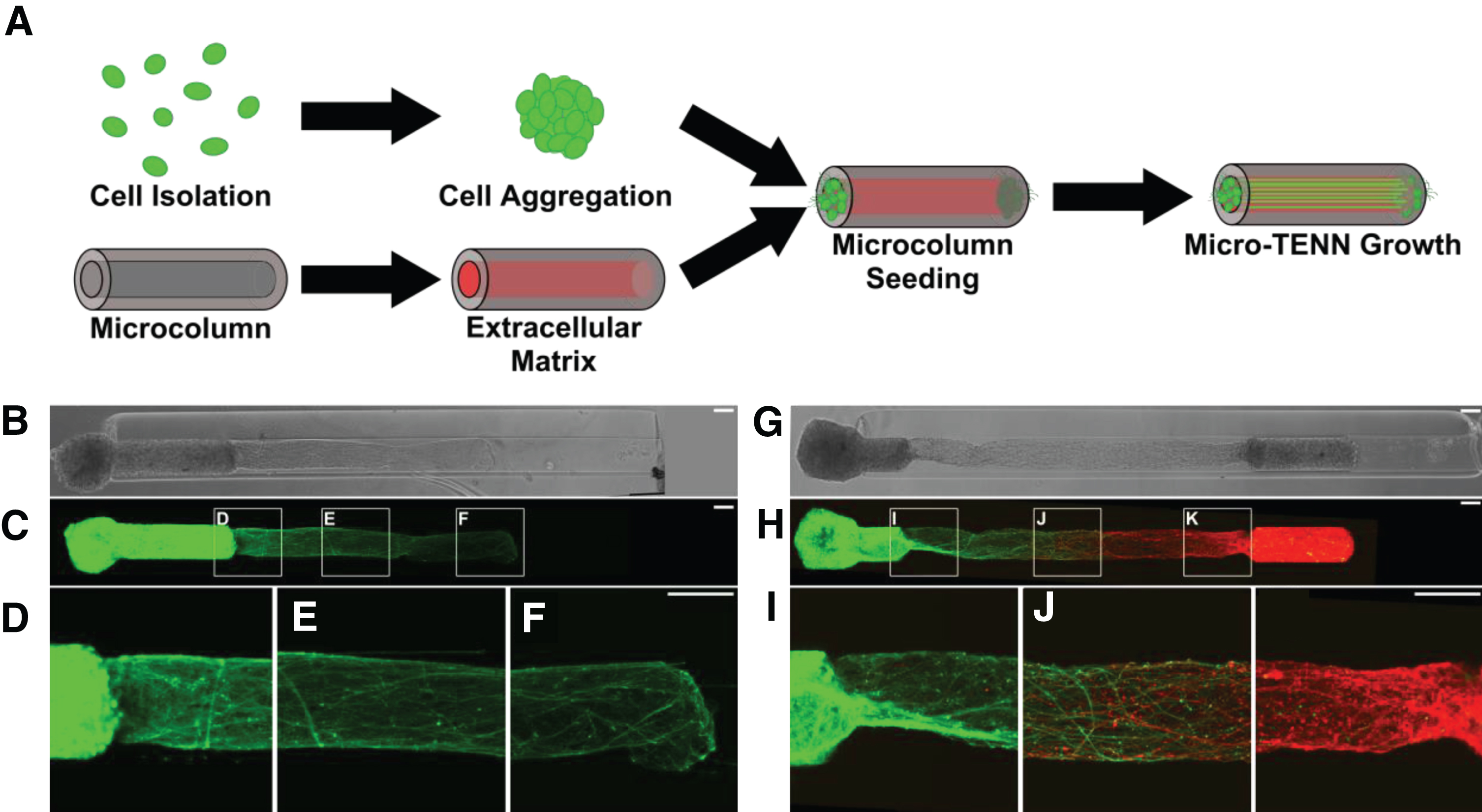
Various neural tissue-engineering tools have been created to model and study the development of neuronal networks in vitro. Among them are micro-tissue engineered neural networks (micro-TENNs), which are three-dimensional (3D) living constructs comprised of long-projecting axonal tracts and discrete neuronal populations within a microscopic, hollow hydrogel cylinder (microcolumn) filled with an extracellular matrix (ECM) [1]. Preformed clusters of neuronal cell bodies (aggregates) are housed at one or both ends of the microcolumn, with axons growing longitudinally through the hydrogel lumen (Fig. 1). This segregation of long axonal tracts and neuronal cell bodies approximates the network architecture of the central nervous system by replicating the anatomy of gray matter and white matter pathways referred to as the “connectome”. Micro-TENNs can be fabricated with a range of neuronal subtypes and physical properties, yielding a controllable yet biofidelic microenvironment for studying 3D neural networks in vitro. As such, micro-TENNs are being developed in parallel as (1) self-contained, bioengineered implants to reconstruct compromised pathways in the brain, and (2) biofidelic test-beds for studying various neuronal phenomena (e.g. growth, synaptic integration, circuit development, pathological responses) [1–5]. Towards the former, prior work has shown that micro-TENNs are capable of survival, maintenance of architecture, neurite outgrowth, and host/implant synaptic integration out to at least 1 month following implant in adult rats [3–6].
Fig.1
Micro-TENNs as living, 3D neuronal-axonal constructs. (A) Micro-TENNs are fabricated in a three-step process. Neurons are isolated and forced into spherical aggregates via gentle centrifugation (top). Simultaneously, single-channel microcolumns are cast from hydrogel to a predetermined inner and outer diameter and filled with an extracellular matrix (ECM) comprised of collagen and laminin (bottom). Next, ECM-filled microcolumns are seeded with either 1 aggregate or 2 aggregates to form either unidirectional or bidirectional micro-TENNs, respectively. Micro-TENNs are then grown in vitro. (B) Phase microscopy image of a unidirectional, GFP-positive micro-TENN at 5 days in vitro (DIV). (C-F) Confocal micrograph of same micro-TENN from (B). Axons can be seen projecting from the neuronal aggregate (D) and extending through the ECM-filled microcolumn (E, F). (G) Phase micrograph of a bidirectional micro-TENN at 5 DIV. The two aggregates have been individually transduced to express GFP (left) and mCherry (right), allowing for identification and monitoring of aggregate-specific processes. (H-K) Confocal micrograph of the micro-TENN from (G), showing axons projecting from each aggregate (I, K) and growing along each other (J). Scale bars: 100 μm.
To advance micro-TENNs’ capabilities as an in vitro testbed and/or to rebuild the damaged connectome, one of our design goals is to develop a computational platform that can be used to design and optimize micro-TENNs for specific performance goals. To be able to investigate neuronal growth, neurite extension, and the formation of synaptic connectivity at the distal ends, we need a simulation framework capable of generating large-scale unidirectional and bidirectional axonal outgrowth with realistic morphologies. The applications of this computational framework for micro-TENNs include: (i) the ability to study processes involved in outgrowth and structural integration in 3D microenvironments; (ii) aid in the design and optimization of functional characteristics and predict performance (e.g., output for a given input); (iii) simulate detailed neuron morphologies and anatomically-relevant neuronal-axonal networks to study connectome-level functional connectivity via spiking or compartmental network modeling. Combining the anatomical simulation results and the study of functional connectivity will increase our ability to understand and predict the neurophysiological characteristics and network-level activity in micro-TENNs.
There are two major approaches to simulate neuronal development: construction algorithms and biologically-inspired growth processes [7]. Construction algorithms aim to reproduce the shape of real dendritic trees from distributions of shape parameters [8, 9]; however, this approach lacks the insight into any underlying biophysical mechanisms, such as the influences on morphological development caused by different neuronal types [10], a neuron’s intracellular environment and interaction with other neurons. Stochastic growth models, which provide a description of the growth process based on probabilistic growing events [11–14], are a popular approach under construction algorithms. On the other hand, biologically-inspired growth processes are based on a description of the underlying biophysical mechanisms of the dendritic development [10,15]; studies have been conducted with various aspects of development, such as cell migration [16], neurite extension [17], growth cone steering [18, 19] and synapse formation [20].
In this paper we present an ad-hoc, phenomenological growth model built upon the diffusion principle, which incorporates the stochastic process to reproduce the shape of micro-TENN tissue. In that sense it belongs to the construction algorithms, however it does not rely on experimentally determined shape parameters. Our approach uses the 3D diffusion equation imposed with various rules for individual neuronal growth, such as the actions of neurite extension, branching, turning and aggregation/bundling.
2Methods
2.1Micro-TENN fabrication and experimental measurements
Micro-TENNs were generated as previously described [4]. Briefly, agarose (3% w/v) was cast in a custom-designed acrylic mold to yield microcolumns with an outer diameter of 345 or 398 μm and inner diameter of 180 μm. Microcolumns were UV-sterilized and cut to a specified length before the lumen was filled with an ECM comprised of rat tail collagen 1 (1 mg/mL) and mouse laminin (1 mg/mL) adjusted to a pH of 7.2–7.4 (Reagent Proteins, San Diego, CA). To create the neuronal aggregates, embryonic day 18 (E18) cortical neurons were isolated from rodents and dissociated. The resultant single-cell suspensions were added to custom PDMS pyramidal wells and centrifuged at 200 x g for 5 minutes to force the cells into spheroidal aggregates. Following 24 h incubation at 37°C/5% CO2, aggregates were seeded within the microcolumns to generate unidirectional (with one aggregate) and bidirectional (with one aggregate at each end) micro-TENNs. Micro-TENNs were then grown at 37°C/5% CO2 with half-media changes every 48 hours. To fluorescently label aggregates, adeno-associated virus 1 (AAV1) was sourced from the Penn Vector Core (Philadelphia, PA), packaged with the human synapsin 1 promoter and either green fluorescent protein (GFP) or the red fluorescent protein mCherry, and added to the pyramidal wells containing the aggregates (final titer: ∼3 ×10¹⁰). Aggregates were kept at 37°C, 5% CO2 overnight before being seeded in micro-columns as described.
During the design and early development of the model, unidirectional and bidirectional micro-TENNs were generated with approximately 15-30E3 neurons per aggregate and lengths ranging from 2.0-9.0 mm (n = 39), with growth rates analyzed as described [5]. To identify aggregate-specific axons over time, a set of 3.0mm-long, bidirectional “dual-color” micro-TENNs were simultaneously generated such that one aggregate expressed green fluorescent protein (GFP) while the opposing aggregate expressed mCherry (n = 6). Finally, for quantitative validation of the growth model, 2.0mm-long, unidirectional micro-TENNs were transduced to express GFP and generated with approximately 20E3 neurons per aggregate (n = 6) or 8.0E3 neurons per aggregate (n = 6) for characterization as described below. Micro-TENNs were imaged under phase contrast microscopy (magnification: 10x) at 1, 3, 5, 8, and 10 days in vitro (DIV) using a Nikon Eclipse Ti-S microscope paired with a QIClick camera and NIS Elements BR 4.13.00 (National Instruments). In addition to phase contrast microscopy, the bidirectional dual-color micro-TENNs were imaged at 1, 2, 3, 5, and 7 DIV using a Nikon A1RSI Laser Scanning confocal microscope paired with NIS Elements AR 4.50.00.
To quantify micro-TENN growth rates over time, the longest identifiable axons were measured from phase images at each DIV using ImageJ (National Institutes of Health, MD). Lengths were measured from the leading edge of the source aggregate (identified at 1 DIV) to the neurite tip, and growth was measured until axons from the aggregate either spanned the micro-TENN length (unidirectional) or began to grow along axons from the opposing aggregate (bidirectional). Growth rates were averaged at each timepoint to obtain a growth profile for unidirectional micro-TENNs with 20E3 and 8.0E3 neurons/aggregate. The peak growth rates for each group were compared using an unpaired t-test, with p < 0.05 set as the baseline for statistical significance.
To characterize axonal density with respect to cell count, phase images of unidirectional micro-TENNs with either 20E3 (n = 6) or 8.0E3 (n = 6) neurons/aggregate at 5 DIV were imported into ImageJ. 10-μm long rectangular regions of interest (ROIs) spanning the inner diameter (final ROI dimensions: 180 μm x 10 μm) were taken at 50% and 75% of the micro-TENN lengths. The axon density at these two locations was quantified as the percentage of the ROI populated by axons. Densities were averaged for the 20E3 and 8.0E3 groups and compared at each location via unpaired t-test with p < 0.05 as the baseline for significance. All data presented as mean±s.e.m.
To characterize axon distribution, unidirectional micro-TENNs were fabricated and labeled with GFP (n = 5). At 10 DIV, micro-TENNs were gently drawn into a 22-gauge needle and vertically injected into a block of “brain phantom” agarose (0.6% w/v). Micro-TENNs were injected such that the aggregate was ventral with axon tracts projecting downward. Post-injection, micro-TENNs were imaged on a Nikon A1RMP+multiphoton confocal microscope paired with NIS Elements AR 4.60.00 and a 16x immersion objective. Micro-TENNs were imaged with a 960-nm laser, with sequential 1.2 μm-thick slices taken along the longitudinal axis (i.e. X-Y projections along the micro-TENN length). Post-imaging, the X-Y projections were used to generate a 3D reconstruction of the micro-TENN; cell bodies, axon bundles, and single axons were then manually identified via co-registration of the X-Y projections and 3D structure.
2.2Computational model development
This framework aims to emulate the growth and bifurcation of micro-TENN neurons by using simple diffusion principles. It avoids most of the underlying biological complexity (due to the lack of external guiding molecular cues) by considering only a few key parameters. Each tip of each neuron is considered as a diffusion source in free space. The elongation and the growth direction of each of the neurites in the model are guided by the contribution of the concentration gradients generated by of the rest of the neurite tips. The motivation for using a concentration gradient to mimic the growth behavior of neurons comes from our experimental observations and from various approaches in the literature. Mathematically, the concentration gradients help drive bundling, and from our experiments we see that axons bundle together as shown in Fig. 1. In addition, in the real brain, bundling of axonal fiber tracts is shown by diffusion tensor imaging [22]. The goal of micro-TENNs is to eventually be considered “replacement” fiber tracts that could be implanted. In both cases of real fiber tracts and micro-TENNs, bundling is observed suggesting an attractive mechanism that we can capture using a concentration gradient approach. Furthermore, it is known that axons have growth cones which are sensitive to various stimuli [23] that create attractive forces. Our model is a phenomenological construct of these ideas that run in a fast fashion ignoring the detailed molecular aspects but focusing on capturing the desired morphology. The bifurcation of the neurites is assumed to be a stochastic process, i.e., branching is associated with a time dependent probability function at each node. All of the tips of the neurite tree are assumed to participate in the extension and branching process; furthermore, extension and branching of each node are modeled as independent processes. This has computational advantages such as improved speed and ability to parallelize on a large scale.
The model uses a continuous space/discrete time approach to allow freedom in the outgrowth direction and elongation. Space is bounded by the inner diameter of the hydrogel micro-column, the diameter and length of the tubular hydrogels, 180 μm and 2 mm respectively, are based on experiments previously performed by the Cullen Lab [1, 3]. In the micro-TENNs, axonal extension is measured approximately every two days; as such, the size of the fixed time interval of the model is 1% of this two-day interval (i.e., 28.8 minutes). In each time step, each individual axonal tip may: (i) extend, (ii) bifurcate into two daughter branches and (iii) change growth direction. In the present implementation, the model uses fixed time steps with functions built upon the diffusion equation and concentration gradients for extension, turning, and branching. The model is developed with the following conditions: the extension rate and turning direction depend on the concentration gradients at the terminal segment of each axon, the extension rate decreases exponentially to zero value [12] as the neurites stop growing due to the limitation of space and essential biochemical factors [14], and branching probabilities grow as a function of the simulation time.
3Extension, tuning and branching
3.1Modeling setup: Diffusion equation and concentration gradient
Many stochastic models of neuronal activity are based on the theory of diffusion processes [24]. In our growth model, the tips of the neurons are modeled as diffusion sources in free space, assuming a constant isotropic diffusion coefficient:
(1)
(2)
The sum of all concentration gradients at each neurite tip is used to help guide the direction of growth for the next time step.
3.2Growth tip position
The coordinates at any given next step of a growth tip (P2) are determined from the coordinates in the previous step (P1), the outgrowth direction (D2), and the extension rate (L); the new position in each time interval is given by:
(3)
3.3Direction of neurite outgrowth
The outgrowth of neurites is a complex process that is far from being fully understood. In actual biological processes, the outgrowth direction of neurites depends on many intracellular and extracellular cues, which may cause large fluctuations in outgrowth directions [22, 23]. Our model assumes that the new outgrowth direction depends on the previous outgrowth direction and on the concentration gradients of the growth tips. For each growth tip, the concentration gradients are normalized, and the new outgrowth direction is given by:
(4)
Fig.2
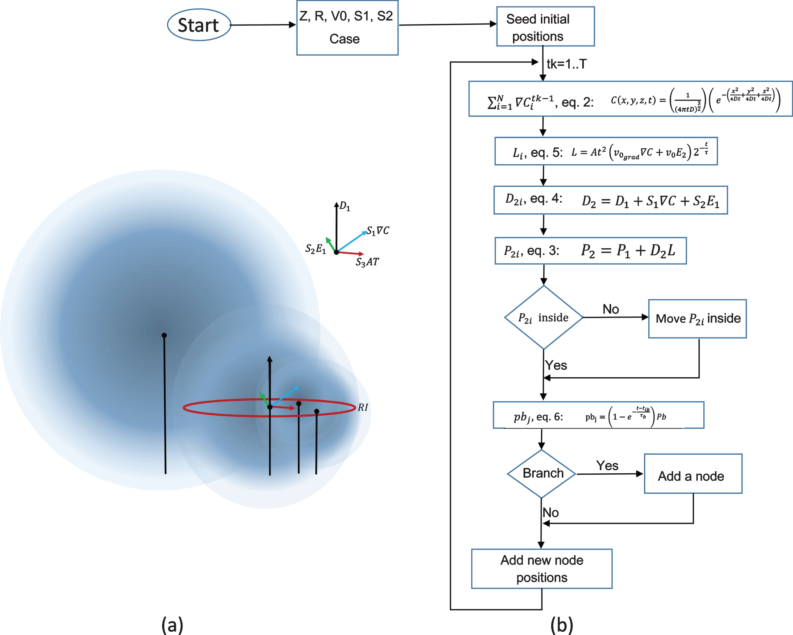
a) Visualization of Equation 4 which shows how the outgrowth of neurites is implemented. The variables are defined in the text. This controlling this term allows change in the magnitude of deviation of the growth direction. b) Pseudocode and schematic of the code implementation requires an initial parameter specification; parameters as sensitivities (S1, Sd1), base growth rate (v0), growth rate based on gradient strength (v0grad), time constant for growth rate (tau), time constant for branching rate (taub), branching probability, bundling (RI), helix formation (chi), total steps, number of cells, inner radius of micro-column among others; these are specified based on experimental/known values. The algorithm then selects among four cases based on chi and bundle values, these cases are used to determine positions after the initial positions. Once calculated, the positions are plotted for its visual inspection and files with coordinates are saved for posterior visualization in Paraview.
3.4Rate of neurite extension
The rate of extension of a neurite (L) may vary considerably and is determined both by the external environment and by the internal state of the neurite in the micro-TENNs [24–31]. In general, the extension rate decreases gradually with increasing distance from the soma [15]; in our model, the description of neurite extension rate follows the trend of experimental growth rate measured in unidirectional micro-TENNs. In each time step, the elongation of a single neurite is represented by the function:
(5)
3.5Branching probability, rate of branching, and growth rate after branching
Neurite branching patterns are complex and show a large degree of variation in their shapes, random branching on the segment indeed results in large and characteristic variations in the structures of the tree; as previous research has highlighted [12, 32], branching is assumed to occur exclusively at terminal nodes. Our model describes branching as a stochastic process: for each time step, for each of the terminal nodes in the growing tree, a branching probability pbj to form two new daughter nodes in a given time interval is assigned. The probability of a branching event at each given terminal node j is given by:
(6)
The time-dependent branching probability pbj of a given terminal node j is dependent on several terms: the steady state branching probability (Pb|t = ∞), simulation time t, the branching time step tib, and a branching time constant τb.
The latter equation assumes that the branching probability of terminal nodes at each time step remains constant for all tips but branching probabilities are growing with the total simulation time; such function was necessary to match the shape of increasing number of dendritic terminal nodes during outgrowth of the micro-TENNs. Whenever a branching event takes place, two daughter terminal nodes are instantaneously added to the end of the existing terminal segment [33], which then becomes an intermediate segment. The stochastic process of branching is also restricted by another random value E3; branching could only occur when both pbj and E3 are greater than a certain value B, the value of B can be determined by the branching probability from experimental data.
The growth rate of the generated trees is closely related with segment outgrowth direction and extension and we only consider the extension distance in the axis direction as the growth distance; therefore, the growth rate is determined by the difference between the z components of the nodes. In the model, we force the growth cones to extend preferentially in the axis direction and the turning is relatively small, in this way the segment extension rate is the strongest factor to determine the growth rate. Estimates of v0, and τ were obtained from the experimental growth rate and the experimental tuning of the elongation parameters which involves a comparison of the experimental and model segment extension rate.
As stated above, with the current implementation the branching probability increases with simulation time and the steady-state branching probability Pb and time constant τb are supposed to be extracted from experimental images. By controlling the values of Pb and τb, we have control over the morphology of the simulated neurites, since Pb controls the branching density and τb controls how early in the process branching begins, e.g., in the extreme case of Pb = 0 we can generate a morphology with no branching.
4Additional functions, parameters and features
4.1Radial constraint
Micro-TENNs are grown within miniature tubular hydrogels experimentally, in the simulations the outgrowth process is also restricted within the tubular space (in this particular case, 180 μm in diameter [1, 3]); however, the model allows different simulation radii to be employed. At each time step, the radial components of all the terminal nodes are tracked, if a radial component of a given node does not satisfy the tubular constraint, the node will be re-oriented to stick on the tubular wall.
4.2Overlap avoidance
The branches and extensions of neighboring neurites often target a shared or adjacent position, i.e., many of the neurites are competing for space and avoiding overlap. Space competing is achieved as a result of the growth based on the concentration gradients explained above. At the same time, overlapping is avoided by checking the distance from the new positions to the surrounding existing segment tips; the model re-orients the growth direction whenever the extended position is sufficiently close to others.
4.3Bundling and helicity
One more feature included in the model is the capacity to accommodate fiber bundling. This is achieved by including an attraction term, i.e., the new position in each time interval becomes:
(7)
Helicity is another feature that was introduced to the model aiming to reproduce observed experimental micro-TENN morphologies. Very often, single axons and axonal bundles once reaching the inner wall of the micro-column, form a helix (Fig. 1); our model allows control over both the slope of the helix formed by an axon (or axonal bundle), as well as its helicity (handedness).
4.4Parameter tuning
Finding a best fit of the model-generated neuronal morphologies for an experimental data set requires an iterative comparison of experimental and model shape properties. When tuning the parameters of the model, some can be directly related to properties of the experimental data or images and can be obtained from them, e.g., the time step is selected to be 0.02 days, based on actual experimental extension measurements (see Results section). Similarly, parameters as v0grad, v0, and τ, which predict the growth rate in axis direction, are susceptible to the same strategy. Noticeably, since v0 can be/is extracted from the experimental data, the selection of the value of the diffusion coefficient (D) is guided by the restriction:
(8)
Other parameters as τb, Pb and S3, govern the branching and fully determine the topological structure of the generated trees, they are directly related to segment branching rate which can also be inferred/estimated from the experimental observations.
Axon growth and bundling along the tube
Slices of the model-generated morphologies were analyzed with ImageJ using the analyze tool after contrast filter/tuning to count to axons and measure the occupied areas. Individual axon areas were divided by the total area in each slice and the resulting ratios for each RI were analyzed as frequency distributions.
Implementation, scaling and computational performance
The code was implemented in Python 2.7-3, even though Python is not recognized as a fast computing language the runtimes are not excessive and the simulations can be performed on standard/modern computers. The algorithm (Fig. 2b) employed by our model is scalable; simulations were performed for 100, 1000 and 10000 cells for the unidirectional micro-TENN with diameter 180 μm and length 2 mm with runtimes were 1.99, 28.93 and 1500.45 seconds, respectively. The simulations were carried out on a laptop (Windows 10 Enterprise 64, Intel i7-7700HQ CPU @ 2.80 GHz, 2801 Mhz, 4 Cores, 16GB DDR3 RAM), all code with is freely available at: https://github.com/PSUCompBio/GrowthModel.
5Results
5.1Examples of micro-TENNs morphologies
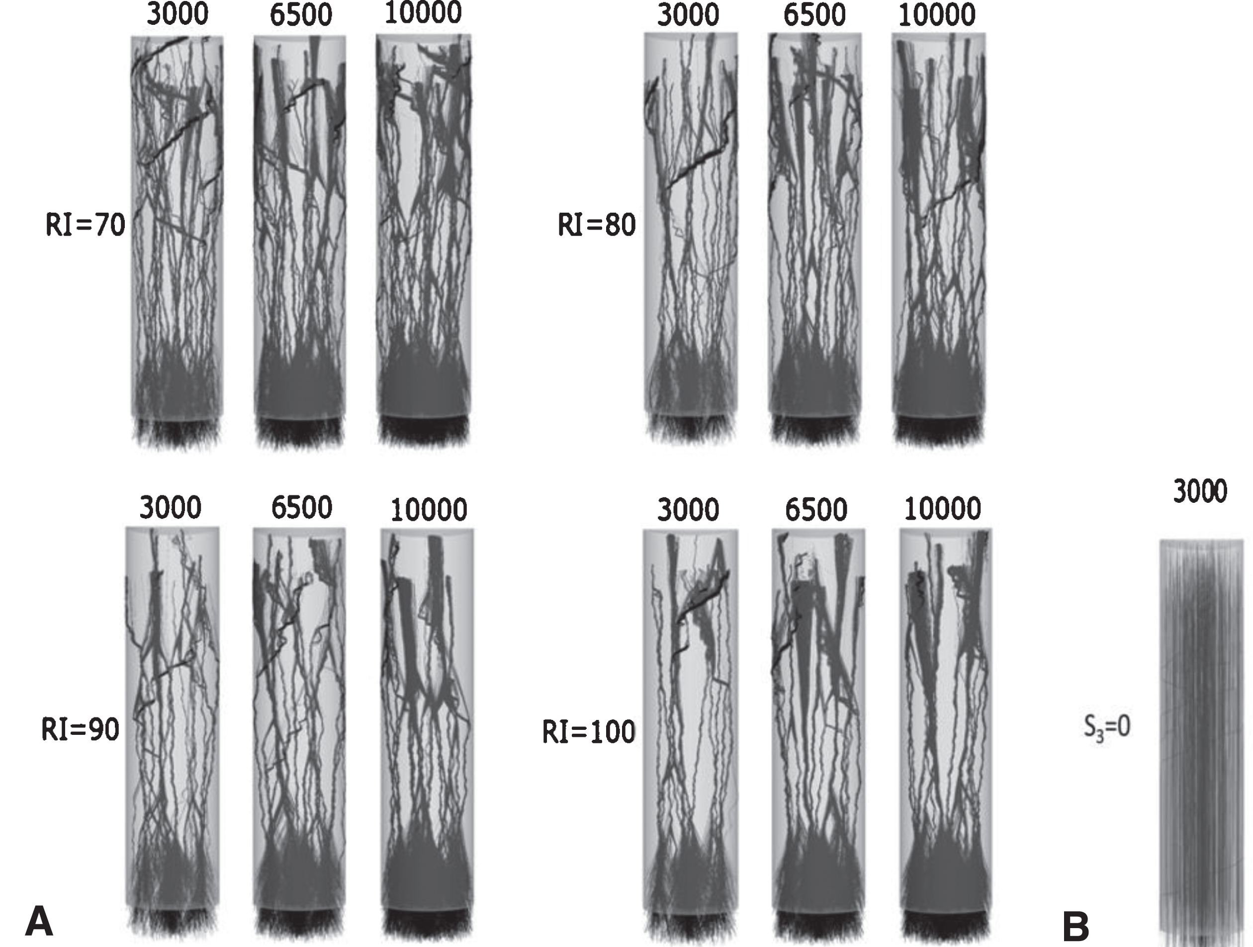
The model simulates satisfactorily the growth processes for unidirectional and bidirectional micro-TENNs when grown to 2000 μm. Variation of model parameters like sensitivity to attraction (S3) and radius of influence (RI) allows us to generate/reproduce different morphologies seen in experimental setups. Figure 3a shows various unidirectional morphologies modelled for micro-TENNs seeded with 3000, 6500 and 10000 cells; it demonstrates how different values of these parameters control the morphologies, e.g., S3 takes continuous values between zero and one, with S3 = 0 corresponding to no bundle formation and S3 = 1 corresponding to tight bundle formation (Fig. 3b and 3a respectively). Higher RIs show fewer bundles for each cell density (Fig. 3a).
Fig.3
Example of unidirectional model-generated micro-TENN morphologies: (A) Twelve morphologies for micro-TENNs of length L=2000 μm and radius R=180 μm, number of seeded cells 3000, 6500 and 10000, and RI=70, 80, 90 and 100 μm, respectively. S3 = 1 causes tight bundle formation. (B) S3 = 0 guarantees no bundle formation.
The case of bidirectional morphologies is presented in Fig. 5, S3 = 0 ensures no bundle formation in spite of the denser setup (Fig. 5) while intermediate values of S3 show not so compact bundles (Fig. 4).
Fig.4
Example of unidirectional model-generated micro-TENNs: Micro-TENNs of length = 2000 μm and radius R = 180 μm, number of seeded cells 3000, 6500 and 10000, and RI = 90 μm. Here S3 = 0.75, bundles are not compact.
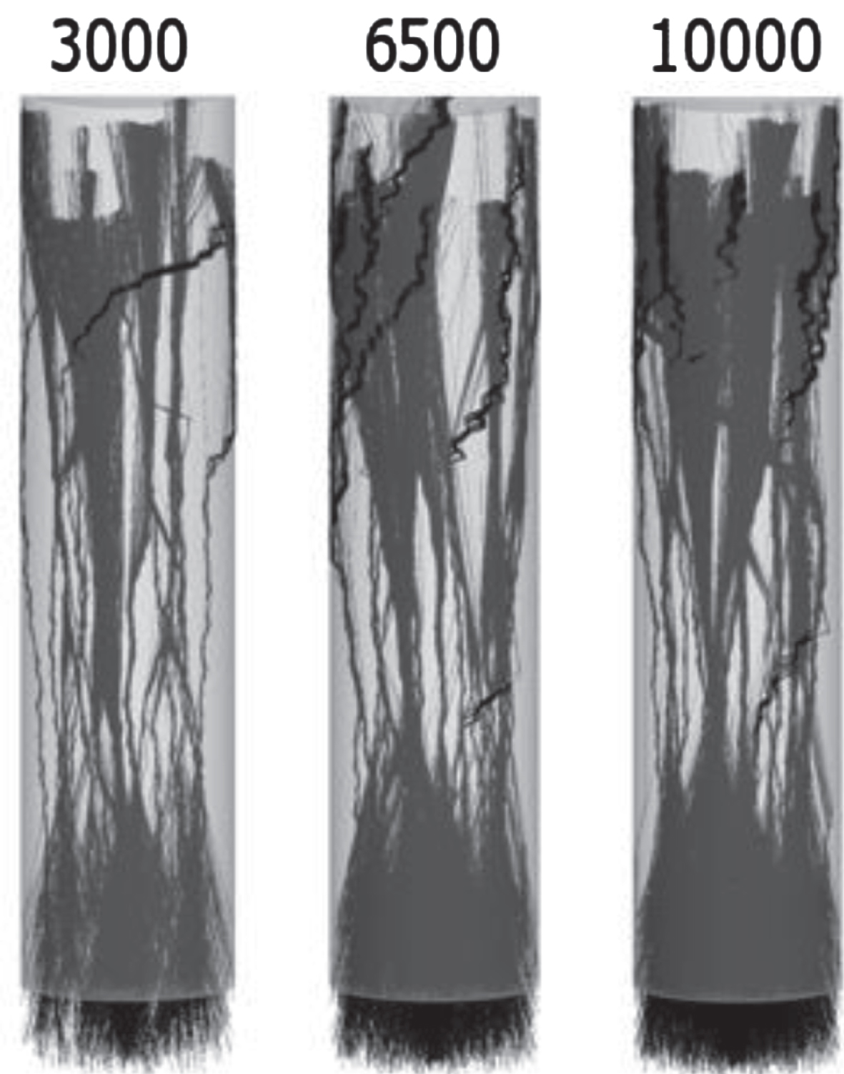
Fig.5
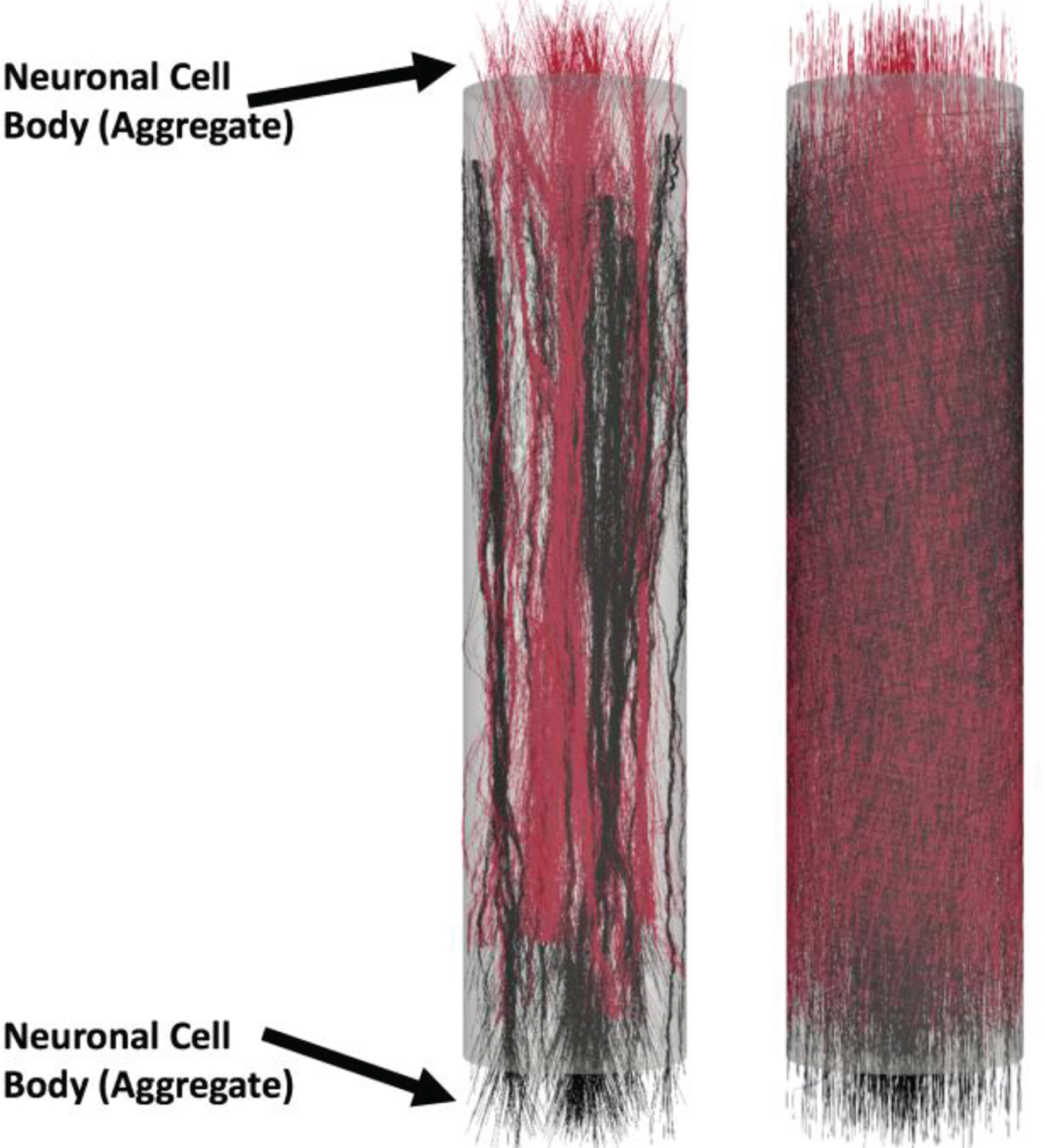
Example of bidirectional model-generated micro-TENNs: Analogously to the unidirectional case, the model can generate bidirectional morphologies. The micro-TENNs have length L=2000 μm and radius R=180 μm, the number of seeded cells is 3000. Here S3 = 1 and RI= 90 μm shows bidirectional axonal bundle formation (left), in the case S3 = 0 no bundles are formed (right). Neuronal cell bodies (aggregate) are labeled on each end but are hidden for clarity.
5.2Experimental calibration of axonal growth rate
Growth rates were computed from the model and compared to those measured from experimental images (Fig. 6a,b) of unidirectional micro-TENNs of approximately 8000 and 20000 neurons; rates are not statistically different (Fig. 6c,d). The optimized parameters, v0 = 15, v0grad = 0.008 and E2 (a random uniform value between 0.8 and 1) provided an excellent fit with the experimental data. The results show that extension rates increase up to three DIV and then decrease as the distance from the soma augments, the same trend can be seen for both the unidirectional and bidirectional growth rates (Fig. 6e,f).
Fig.6
Calibration of simulated growth rates in vitro. (A) Phase images of a unidirectional micro-TENN with approximately 8,000 neurons at 1, 3, and 5 DIV. (B) Phase images of a unidirectional micro-TENN with approximately 20,000 neurons at 1, 3, and 5 DIV. Both micro-TENN groups exhibited rapid axonal growth over the first few DIV. Scale bars: 100 μm. (C) Growth rates from both micro-TENN groups at 1, 3, and 5 DIV. Micro-TENNs with ∼20,000 neurons/aggregate exhibited qualitatively faster growth rates than those with ∼8,000 neurons/aggregate, although there were no statistically significant differences in growth rates. (D) Axon density at 5 DIV across the two groups at 50% and 75% along the micro-TENN length (as illustrated in (B)), quantified as the percentage of the microcolumn channel occupied by axons. Micro-TENNs with ∼20,000 neurons/aggregate showed higher axon densities than those with ∼8,000 neurons/aggregate, although this was only significant at 50% along the micro-TENN length (*** = p < 0.001). (E) Experimental versus model growth rate for unidirectional micro-TENN with 8,000 neurons. (F) Experimental versus model growth rate for unidirectional micro-TENN with 20,000 neurons.
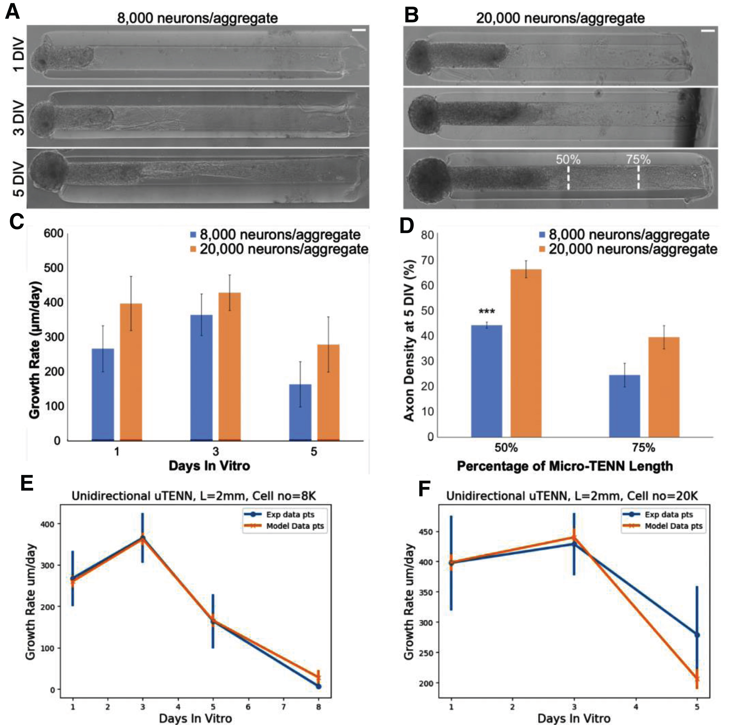
Figure 7a shows a 3D-reconstruction of a unidirectional micro-TENN at 10 DIV. Four corresponding slices were extracted for cross-sectional comparison to the computed results. Figure 7b–e show each slice marked with arrows to distinguish between neuronal cell bodies, axon bundles, and single axons. In order to compare morphologies, we use two model-generated X-Y projections along the Z-axis (Fig. 8) that resulted from a micro-TENN simulation (inner radius 180 μm, length of 2 mm, number of seeded cells 20,000). The model generates realistic morphology with single axons and axon bundles along the inner wall comparable to the experimentally reconstructed morphology in Fig. 7.
Fig.7
(A) 3D reconstruction of a unidirectional, GFP-positive micro-TENN at 10 DIV. (B–E) X–Y projections of the micro-TENN from (A) at the sections outlined in red. Orientation of the z-axis (positive) is into the page. Neuronal cell bodies (arrows) can be seen near the aggregate region in (B), from which axonal bundles (triangles) project and split into individual axons (caret). Scale bars: 200 μm (A); 50 μm (B).
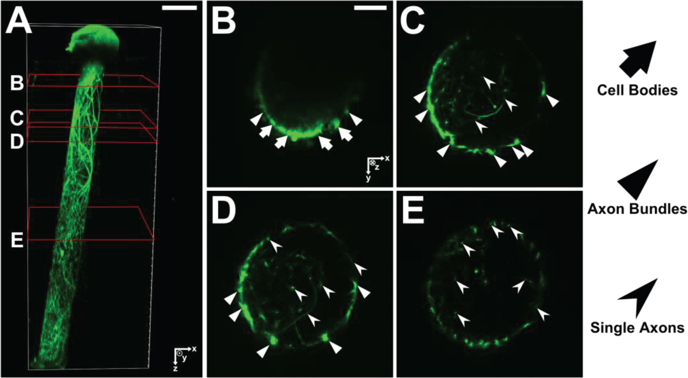
Fig.8
Model generated morphology of a unidirectional micro-TENN. (A) X–Y projection at Z = 910 μm; (B) X–Y projection at Z = 1380 μm. Inner diameter 180 μm, length 2 mm and approximately 20,000 neurons.
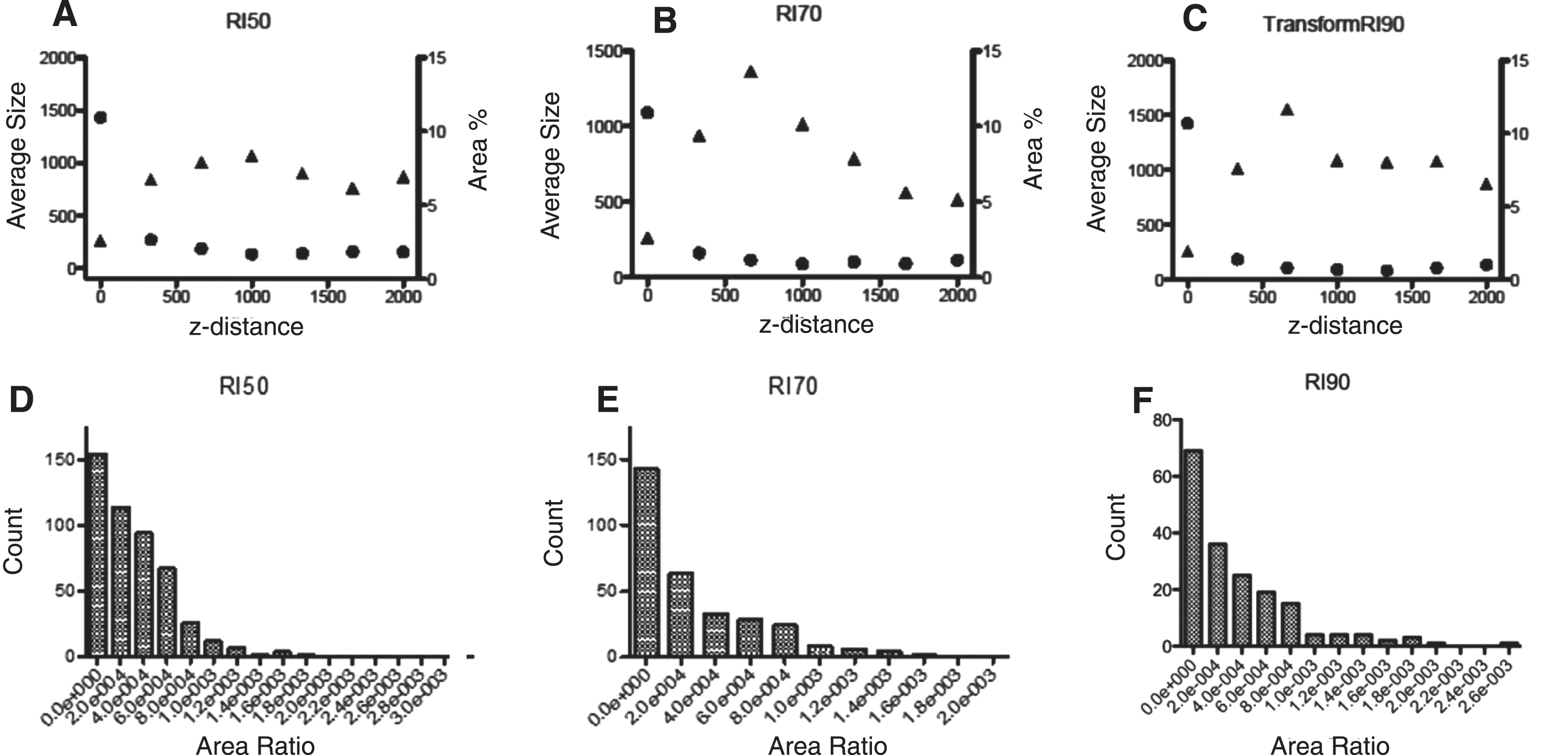
From different slices along the z-axis in our simulations we analyzed the percentage of area covered in the slice which serves as descriptor of the axon bundling along the tube. It should be noted that according to the models, the highest average size for the axons is reached between 660 μm and 990 μm in z-direction, i.e., where the bundles are bigger along the tube. Experimental confirmation is needed to test our observations. Different combinations of simulation parameters create particular micro-TENN morphologies, in an attempt to qualitatively characterize them we measured the area ratio of the bundle/micro-TENN cross sections at 5 equidistant z-values along the micro-TENN for 3 different RI (Fig. 9d,e,f). The resultant distribution for each RI is distinct and allows qualitative comparison between simulation morphology data and experimental microscopy micro-TENN data when it becomes available. The most abundant type are the smaller ratio areas (individual axons), both RI 50 and 70 have bigger counts of this type than RI 90; on the other hand, RI 90 presents the bigger area ratios (bundles). These results reflect the effect of RI in bundle formation using our model.
Fig.9
Bundle % area coverage (circles) and average bundle size (triangles) as a function of length in the micro-TENN. (A) RI = 50; (B) RI = 70; (C) RI = 90. Combined area ratio distributions from five z-cross sections from simulated microTENNs with (D) RI = 50, € RI = 70 and (F) RI = 90, respectively. The distinct distribution correspond to distinct microTENN morphologies.
6Discussion
As a neural network model, micro-TENNs allow systematic interrogation of different contributors to neuronal growth and development in a three-dimensional, anatomically-relevant environment. By providing precise control of the neuronal subtypes within the engineered aggregates, the extracellular matrix and milieu, as well as the potential presence of supporting glial cells, the micro-TENNs provide an ideal platform for the evaluation of interplay between intrinsic and extrinsic mechanisms of neuronal growth and neurite extension. For instance, the 3D biomaterial columnar encasement provides an unprecedented engineered environment to study the multi-faceted and often synergistic contributions of haptotactic [mediated by ECM (e.g., laminin, collagen) and cell-surface ligands (e.g., cadherins, L1)], chemotactic [mediated by growth factor gradients (e.g., nerve growth factor, glial derived neurotrophic factor) that can be attractive or repulsive], and mechanotactic [dictated by substrate geometry (e.g., curvature) and mechanical properties (e.g., stiffness)] on axonal outgrowth and pathfinding [34, 35]. To date, micro-TENNs have been generated with lengths ranging from 1–30 mm, and inner diameters as small as 160 μm [4]. Moreover, the introduction of “actuator proteins” such as channelrhodopsin-2 (a light-sensitive ion channel for optically-induced neuronal stimulation) and/or activity markers such as the fluorescent calcium reporter GCaMP also provide a range of techniques to both modulate and monitor neuronal activity within the micro-TENN over time [5]. This controllability makes micro-TENNs an ideal test bed for eliciting and studying different neuronal phenomena under a range of experimental conditions, all within a three-dimensional architecture more similar to the native brain than traditional 2D cultures or randomly organized 3D cultures.
Existing models have been applied to study neuronal development in vivo, generally in the presence of molecular cues and under no specific geometric restrictions]. Those conditions differ from the experimental growth conditions of micro-TENNs, in which some gradients of external molecular cues are missing e.g., the matrix is not neural tissue, and the growth space is a narrow tubular environment. Moreover, most of the existing models include complex growth mechanisms, leading to large computational cost. To compliment these previous efforts, there is a need for computationally inexpensive models (due to the large populations of neurons) capable of capturing the morphology of axonal growth within geometrical restrictions, including important behaviors/features as neurite branching and axonal bundle formation/fasciculation as the one described here.
The presented model is designed to capture some of these important basic biological principles of neuronal development and axonal outgrowth in vitro: the competition for space and resources between growing tips, the formation of bundles, chirality, the dependence of branching probability on the growth time, and the deceleration of the growth rate over time. The growth rate values in our model successfully reproduce those in experimental data and the implementation is a fast/computationally-inexpensive ad-hoc stochastic process-based simulation framework for the generation of large-scale unidirectional and bidirectional neuronal networks with realistic neuronal-axonal morphologies. Micro-TENN design and optimization can be assessed prior any experiment with this tool. After fine-tuning of the parameters described in the methods section, the simulations can help in the decision making for the different experimental setups under study.
The main advantage of the model is its conceptual simplicity. It is built on basic principles, yet it can generate various complex morphologies observed experimentally (Figs. 3–7) with only a few parameters from de novo conditions. Another major advantage is the computational speed; the solution of the diffusion equation for each tip is explicit and analytic, thus removing the necessity for a numerical solution for the concentration and the concentration gradients. This makes the model fast and computationally cheap, particularly for a large number of growing neurons. Furthermore, each growth tip represents a separate process, allowing for parallelization and additional speed up of computational.
On the other hand, a limitation to the model is the introduction of parameters that cannot be extracted directly from experimental data, sometimes due to the data resolution or simply to an inability of reliably quantifying certain experimental aspects. The parameter space they form has to be scanned for values that allow realistic neuronal morphologies. The actual implementation lacks of chemical cues in the unidirectional case, such cues are imperative to reproduce completely the experimental models; while the model/implementation allows for additional attraction/repulsion and guidance terms to be introduced, employing direct extrapolation from in vivo growth models is challenging due to its chemically complex nature and the potential pitfalls derived form chemical kinetic/gradient theory.
6.1Future work
One major objective of further building/developing the Bidirectional Growth Model is to generate simulations of detailed neuron growth patterns to ultimately enable the study of functional connectivity that our research group has begun [36]. For instance, these neuronal growth patterns could be used as the input of a spiking model to study the firing patterns within micro-TENNs. The framework could also be used to extract detailed connectivity information in scenarios following implantation; patterns at the distal ends of micro-TENNs upon integration with the host brain neurons could be modeled/described/anticipated.
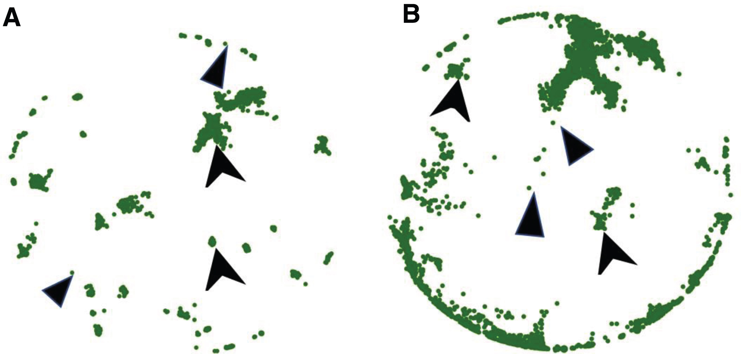
The neuronal growth patterns provide the information for searching locations of synaptic connections and help to establish the spiking network simulation. In biological neuronal networks, synapses form in regions where tissues are in sufficiently close proximity and synaptic connectivity is estimated (proximity criterion of 0.5 μm). According to experimental design, synapses occur close to the cells aggregates, which are in the 100 μm range from each end of the micro-TENNs. Figures 10A/2B give examples of the locations of these synaptic sites where high connectivity is presented. Further development of the model could introduce additional guidance and attraction/repulsion molecular cues, once such experimental information is available, thereby systematically adding complexity and the ability to capture synergistic and/or competing features of intrinsic and extrinsic growth parameters.
Fig.10
Growth pattern and synapses examples. Illustration of synaptic formation close to the cells aggregate. The spheres indicate the synapses location. We consider that a synapse is formed when 2 fibers are closer than a threshold distance of 0.5 μm. Synapses occur close to the aggregate (within 100 μm). The connectivity information is extracted for the spiking network simulation. (A) The output image of the model: synaptic formation in bidirectional micro-TENNs without axonal bundles. (B) The output image of the model: synaptic formation in bidirectional micro-TENNs with axonal bundles.

7Conclusion
The neuronal and axonal growth structures obtained through this model provide a complete growth and connectivity pattern within a custom micro-tissue neural network. The model reproduces both the micro-TENN architecture and the axonal growth rate and distribution. This framework will enable further assessment of structural and functional connectivity, for instance an analysis of synaptic integration that happens close to the aggregate or even outside the micro-column. The extracted information of synaptic connectivity close to the aggregate and the synapse at distal end of micro-TENNs will be the topic of a future functional connectivity study. We intend to build on this model in order to better understand the spiking network properties of micro-TENNs as so-called “living electrodes” for neuromodulation as well as anatomically inspired constructs for white matter pathway reconstruction.
Acknowledgments
Research reported in this publication was supported by the National Institutes of Health through the Brain Initiative [U01-NS094340 (Cullen & Kraft)], the National Science Foundation through a Graduate Research Fellowship [DGE-1321851 (Adewole)], and National Science Foundation CAREER award [1846059 (PI: Kraft)]. Computations for this research were performed on the Pennsylvania State University’s Institute for Computational and Data Sciences Advanced CyberInfrastructure (ICS-ACI).
References
[1] | Cullen D.K. , et al., Microtissue engineered constructs with living axons for targeted nervous system reconstruction, Tissue Eng. Part A 18: ((2012) ), 120817094501006. doi: 10.1089/ten.tea.2011.0534 |
[2] | Harris J.P. , Struzyna L.A. , Murphy P.L. , Adewole D.O. , Kuo E. , Cullen D.K. , Advanced biomaterial strategies to transplant preformed micro-tissue engineered neural networks into the brain, J. Neural Eng. 13: (1) ((2016) ), doi: 10.1088/1741-2560/13/1/016019. |
[3] | Struzyna L.A. , et al., Rebuilding brain circuitry with living micro-tissue engineered neural networks, Tissue Eng. Part A 21: (21–22) ((2015) ), 2744–2756, doi: 10.1089/ten.tea.2014.0557. |
[4] | Struzyna L.A. , et al., Anatomically inspired three-dimensional micro-tissue engineered neural networks for nervous system reconstruction, modulation, and modeling, J. Vis. Exp. JoVE 123: ((2017) ), doi: 10.3791/55609. |
[5] | Adewole D.O. , et al., “Optically-Controlled ‘Living Electrodes’ with Long-Projecting Axon Tracts for a Synaptic Brain-Machine Interface,” bioRxiv, Jan. (2018) . |
[6] | Struzyna L.A. , et al., Tissue engineered nigrostriatal pathway for treatment of Parkinson’s disease, J. Tissue Eng. Regen. Med. 12: (7), 1702–1716, doi: 10.1002/term.2698. |
[7] | Zubler F. , Douglas R. , A framework for modeling the growth and development of neurons and networks, Front. Comput. Neurosci. 3: ((2009) ), doi: 10.3389/neuro.10.025.2009. |
[8] | Ascoli G.A. , Krichmar J.L. , Scorcioni R. , Nasuto S.J. , Senft S.L. , Krichmar G.L. , Computer generation and quantitative morphometric analysis of virtual neurons, Anat. Embryol. (Berl.) 204: (4) ((2001) ), 283–301, doi: 10.1007/s004290100201. |
[9] | Hamilton P. , A language to describe the growth of neurites, Biol. Cybern. 68: (6) ((1993) ), 559–565, doi: 10.1007/BF00200816. |
[10] | Graham B.P. , van A. , Ooyen, Transport limited effects in a model of dendritic branching, J. Theor. Biol. 230: (3) ((2004) ), 421–432, doi: 10.1016/j.jtbi.2004.06.007. |
[11] | Kliemann W. , A stochastic dynamical model for the characterization of the geometrical structure of dendritic processes, Bull. Math. Biol. 49: (2) ((1987) ), 135, doi: 10.1007/BF02459695. |
[12] | Van Pelt J. , DityatevA.E. and UylingsH.B.M., Natural variability in the number of dendritic segments: model-based inferences about branching during neurite outgrowth, J. Comp. Neurol. 387: (3) ((1997) ), 325–340, doi: 10.1002/(SICI)1096-9861(19971027)387:3 < 325::AID-CNE1 > 3.0.CO;2-2. |
[13] | Carriquiry A.L. , Ireland W.P. , Kliemann W. , Uemura E. , Statistical evaluation of dendritic growth models, Bull. Math. Biol. 53: (4) ((1991) ), 579–589. doi: 10.1007/BF02458630. |
[14] | Villacorta J.A. , Castro J. , Negredo P. , Avendaño C. , Mathematical foundations of the dendritic growth models, J. Math. Biol. 55: (5–6) ((2007) ), 817–859, doi: 10.1007/s00285-007-0113-7. |
[15] | Norton K.-A. , Wininger M. , Bhanot G. , Ganesan S. , Barnard N. , Shinbrot T. , A 2d mechanistic model of breast ductal carcinoma in situ (dcis) morphology and progression, J. Theor. Biol. 263: (4) ((2010) ), 393–406. doi: 10.1016/j.jtbi.2009.11.024. |
[16] | Hely T.A. , Graham B. , Van Ooyen A. , A computational model of dendrite elongation and branching based on MAP2 phosphorylation, J. Theor. Biol. 210: (3) ((2001) ), 375–384, doi: 10.1006/jtbi.2001.2314. |
[17] | Cai A.Q. , Landman K.A. , Hughes B.D. , Modelling directional guidance and motility regulation in cell migration, Bull. Math. Biol. 68: (1) ((2006) ), 25, doi: 10.1007/s11538-005-9028-x. |
[18] | Kiddie D. , McLean D. , Van Ooyen A. and GrahamB., Biologically plausible models of neurite outgrowth, in Development, Dynamics and Pathology of Neuronal Networks: From Molecules to Functional Circuits, 1st ed., vol. 147: . |
[19] | Goodhill G.J. , Gu M. , Urbach J.S. , Predicting axonal response to molecular gradients with a computational model of filopodial dynamics, Neural Comput 16: (11) ((2004) ), 2221–2243, doi: 10.1162/0899766041941934. |
[20] | Maskery S. , Shinbrot T. , Deterministic and stochastic elements of axonal guidance, Annu. Rev. Biomed. Eng. 7: ((2005) ), 187–221, doi: 10.1146/annurev.bioeng.7.060804.100446. |
[21] | Stepanyants A. , Hirsch J.A. , Martinez L.M. , Kisvárday Z.F. , Ferecskó A.S. , Chklovskii D.B. , Local potential connectivity in cat primary visual cortex, Cereb. Cortex 18: (1) ((2008) ), 13–28, doi: 10.1093/cercor/bhm027. |
[22] | Stieltjes B. , et al., Diffusion tensor imaging and axonal tracking in the human brainstem, Neuroimage 14: (3) ((2001) ), 723–735. |
[23] | Goodman C.S. , Mechanisms and molecules that control growth cone guidance, Annu. Rev. Neurosci. 19: (1) ((1996) ), 341–377. |
[24] | Lansky P. , Smith C. , One-dimensional stochastic diffusion models of neuronal activity and related first passage time problems, Trends Biol. Cybemetics 1: ((1990) ), 153–162. |
[25] | Karube F. , Kubota Y. , Kawaguchi Y. , Axon branching and synaptic bouton phenotypes in GABAergic nonpyramidal cell subtypes, J. Neurosci. 24: (12) ((2004) ), 2853–2865. doi: 10.1523/JNEUROSCI.4814-03.2004. |
[26] | Kalil K. , Dent E.W. , Branch management: mechanisms of axon branching in the developing vertebrate Cns,” Nat. Rev. Neurosci. 15: (1) ((2014) ), 7–18, doi: 10.1038/nrn3650. |
[27] | Hjorth J.J.J. , van Pelt J. , MansvelderH.D. and van OoyenA., Competitive dynamics during resource-driven neurite outgrowth, PLoS ONE 9: (2) ((2014) ), doi: 10.1371/journal.pone.0086741. |
[28] | Li G.-H. , Qin C.-D. , A model for neurite growth and neuronal morphogenesis, Math. Biosci. 132: (1) ((1996) ), 97–110. doi: 10.1016/0025-5564(95)00052-6. |
[29] | Suter D.M. , Miller K.E. , The emerging role of forces in axonal elongation, Prog. Neurobiol 94: (2) ((2011) ), 91–101, doi: 10.1016/j.pneurobio.2011.04.002. |
[30] | O’Toole M. , Latham R. , Baqri R.M. , Miller K.E. , Modeling mitochondrial dynamics during in vivo axonal elongation, J. Theor. Biol 255: (4) ((2008) ), 369–377. doi: 10.1016/j.jtbi.2008.09.009. |
[31] | Van Veen M.P. and Van PeltJ., Neuritic growth rate described by modeling microtubule dynamics, Bull. Math. Biol. 56: (2) ((1994) ), 249–273. |
[32] | O’Toole M. , Lamoureux P. , Miller K.E. , A physical model of axonal elongation: Force, viscosity, and adhesions govern the mode of outgrowth, Biophys. J 94: (7) ((2008) ), 2610–2620, doi: 10.1529/biophysj.107.117424. |
[33] | Graham B.P. , Lauchlan K. , Mclean D.R. , Dynamics of outgrowth in a continuum model of neurite elongation,” J. Comput. Neurosci. 20: (1) ((2006) ), 43, doi: 10.1007/s10827-006-5330-3. |
[34] | Gibson D.A. , Ma L. , Developmental regulation of axon branching in the vertebrate nervous system, Development 138: (2) ((2011) ), 183–195. doi: 10.1242/dev.046441. |
[35] | van Ooyen A. , van PeltJ. , and UylingsH., “Modeling Dendritic Geometry and the Development of Nerve Connections,” in Computational Neuroscience, CRC Press, (2000) . |
[36] | Cullen D.K. , Wolf J.A. , Vernekar V.N. , Vukasinovic J. , LaPlaca M.C. , Neural tissue engineering and biohybridized microsystems for neurobiological investigation(Part 1), Crit. Rev. Biomed. Eng. 39: (3) ((2011) ). |
[37] | Cullen D.K. , et al., Microtissue engineered constructs with living axons for targeted nervous system reconstruction, Tissue Eng. Part A 18: (21–22) ((2012) ), 2280–2289. |
[38] | Dhobale A.V. , et al., Assessing functional connectivity across 3D tissue engineered axonal tracts using calcium fluorescence imaging, J. Neural Eng. 15: (5) ((2018) ), 056008. doi: 10.1088/1741-2552/aac96d. |