Towards time-evolving analytics: Online learning for time-dependent evolving data streams
Abstract
Traditional historical data analytics is at risk in a world where volatility, uncertainty, complexity, and ambiguity are the new normal. While Streaming Machine Learning (SML) and Time-series Analytics (TSA) attack some aspects of the problem, we still need a comprehensive solution. SML trains models using fewer data and in a continuous/adaptive way relaxing the assumption that data points are identically distributed. TSA considers temporal dependence among data points, but it assumes identical distribution. Every Data Scientist fights this battle with ad-hoc solutions. In this paper, we claim that, due to the temporal dependence on the data, the existing solutions do not represent robust solutions to efficiently and automatically keep models relevant even when changes occur, and real-time processing is a must. We propose a novel and solid scientific foundation for Time-Evolving Analytics from this perspective. Such a framework aims to develop the logical, methodological, and algorithmic foundations for fast, scalable, and resilient analytics.
1.Introduction
From drilling in an oil ring to managing traffic, from how doctors diagnose a disease to performing financial operations, the growing ability to collect, integrate, store, and analyze massive data fuels scientific breakthroughs and technological innovations. Recently, Machine Learning (ML) models exhibited or even surpassed human-level performance on individual tasks, e.g., Atari games [41] or object recognition [38]. Although these results are impressive, they are obtained from static models incapable of adapting their behaviour over time. As such, this requires restarting the training process each time new data becomes available (a.k.a. stateless retraining). In our dynamic world, this practice quickly becomes intractable for data streams or data, more generally, that may only be available temporarily due to storage constraints or privacy issues. Data streams call for novel stateful systems that adapt continuously and keep learning over time. The urgency of this capacity is all the more remarkable if we consider that, despite the continuous advances in storage technology, already in 2025, the demand for storage will outstrip storage production by one order of magnitude. Seagate predicts that this exponential inflation will require analyzing almost 30% of global data in real-time [37].
Moreover, in a growing number of markets where the demand for products was stable or even linear, the period in which the products are saleable is now short and seasonal. Finally, when changes hit, organizations that employ traditional stateless analytics techniques that rely heavily on historical data discover that their models are no longer relevant, resulting in a performance decrease. COVID-19 is one of those changes. As a consequence of the pandemic, many datasets became useless, causing several Pre-COVID-19 models to be no longer valid (src. Gartner [33] and MIT Tech Review [22]). Indeed, the typical assumption that data points are independent and identically distributed (i.i.d.) holds no longer. Historical data analytics, which counts on i.i.d., is at high risk. This particular non-stationary phenomenon is called concept drift [44].
Streaming Machine Learning (SML) [6] is the most popular stateful system. It incorporates one sample at a time, incrementally updating the model instead of retraining it anew. To cope with the stream’s unboundedness, each instance, once used, is discarded. Moreover, in the SML framework, we can find models that only learn the underlying concept incrementally, without tackling concept drifts (Incremental Learning) and models that use a concept drift detector to adapt their already acquired knowledge to new concepts (SML).
A shared need is emerging for a novel type of Time-Evolving Analytics that:
R1. is not limited to a specific setting, i.e., it does not focus on a specific problem (e.g., only classification), but includes supervised, semi-supervised and unsupervised problems;
R2. makes high-order predictions,11 i.e., exploiting dependence in the sequences that spans multiple time steps and multiple scales from seconds/minutes to months/years;
R3. predicts multiple possible future outcomes., i.e., in a complex and uncertain world, the most probable outcome may be insufficient, and the ability to predict and evaluate the likelihood of each prediction becomes crucial;
R4. continuously adapts to changes, i.e., in a volatile world where data often have statistics that evolve, forgetting or ignoring past data becomes crucial;
R5. learns statefully, i.e., the ability to detect patterns on the fly without the need to store all the data and pass through them multiple times is crucial; ideally, algorithms should learn from one data point at a time before discarding it; and
R6. does not structure the model a priori but allows the number and nature of the parameters to evolve.
As Table 1 shows, there are clear distinctions about each existing model’s type of data. The difference between time series and data streams may be questioned. Indeed, time series may commonly arrive in the form of online data and thus can be treated as a data stream. Another way of seeing it is that data streams may often involve temporal dependence and thus be considered time series. Undoubtedly, the most general scenario is to handle not i.i.d. data stream. Offline Machine Learning deals only with independent and identically distributed data, not addressing neither R4 nor R5. Incremental Learning does not adapt to changes (R4), despite addressing R5. Moreover, while Streaming Machine Learning (SML) and Time-series Analytics (TSA) attack some of these challenges, we are far from a comprehensive solution. SML trains models stateful way [6] (R5) also adapting to concept drift occurrences (R4), i.e., relaxing the assumption that data points are identically distributed but still assuming that there is no temporal dependence. Hence, it does not address R2. In this specific case, the stream takes the name of evolving data stream, containing concept drifts but no (assumed) temporal dependence. On the contrary, TSA considers temporal dependence among data points [10] (R2), but it assumes identical distribution. Thus, it does not address R4. Indeed, every Data Scientist fights these challenges with ad-hoc solutions.
Table 1
Difference between offline machine learning, incremental learning, streaming machine learning, time series analysis, and time-evolving analytics framework
| i.i.d. dataset | i.i.d. data stream | Time-dependent time series | Evolving data stream | Not i.i.d. data stream | |
| Offline Machine Learning | ✔ | ✘ | ✘ | ✘ | ✘ |
| Incremental Learning | ✔ | ✔ | ✘ | ✘ | ✘ |
| Streaming Machine Learning | ✔ | ✔ | ✘ | ✔ | ✘ |
| Time Series Analysis | ✔ | ✘ | ✔ | ✘ | ✘ |
| Time-Evolving Analytics | ✔ | ✔ | ✔ | ✔ | ✔ |
In particular, the contributions of this paper are the following:
We provide empirical evidence using the well-known Electricity dataset [21] that the contemporaneous presence of changes in the data distribution and temporal dependences puts ML, SML, and TSA at risk of being ineffective. In particular, we introduce a new experimental methodology that extends previous analysis [4,50] adding ML, analyzing models’ accuracy over time, and tracking their resource usage.
We envision a new framework (namely, Time-Evolving Analytics) that keeps models (R1) relevant even when changes occur (R4), and real-time processing is a must (R5).
We explain why such a framework has the potential to pave the way for the development of a new generation of sequential models that embed high-order temporal dependence (R2) and predict multiple possible futures (R3) without a fixed model structure (R6).
We indicate the characteristics of a unifying model for Time-Evolving Analytics that does not assume i.i.d. and a unifying methodology that can guide practitioners in systematically addressing the requirements listed above.
The remainder of this paper is organized as follows. Section 2 discusses the need for Time-Evolving Analytics, overcoming the currently existing limitations. In Section 3 we give an overview of the main works about the temporal dependence in time series and data streams. In Section 4, we detail the experiments that support the thesis about the need for a new analytic. Section 5 presents the main challenges and benefits that may arise with Time-Evolving Analytics. Section 6 outlines the desiderata of the envisioned model and methodology. Finally, Section 7 discusses the main takeaways regarding research opportunities and challenges explored throughout the paper.
2.Time for a principled solution
For Computer Science, the 2000s have seen the Big Data industry’s come-of-age and the corresponding scientific field at the intersection of High-Performance-Computing, Databases, and Machine Learning. New technology concepts are formulated and quickly transferred into products. The scientific community struggles to keep the industry’s pace, lingering considerably.
For instance, take the case of nowcasting. The term is a contraction of “now” and “forecasting.” It originates in meteorology, referring to the need for weather forecasts that are time and space specific for periods less than a few hours [47]. However, it is an active research field also in economics [19], epidemiology [24,48], and energy [49], just to cite a few. These forecasts are particularly hard because the i.i.d. assumption hardly holds, multiple temporal dependencies are present, and changes (both in data distribution and the order of the temporal dependency) are frequent. As a result, past data are often of little practical interest (i.e., forgetting them is valid). However, a method can be effective only by selectively remembering recurring patterns and seasonal effects. Moreover, even if the ideal forecast should be crisp, the uncertainty is so high that the only viable solution is to generate alternative predictions with an associated confidence level. Last but not least, nowcasting also means massive flows of observations that we had better process incrementally than in large batches.
We claim that the rapid and ad-hoc solutions appearing on the market22 cannot provide long-term foundations and will fail to adapt models fast enough in the volatile, complex, and uncertain future that awaits us [37]. We argue that academia has a crucial role in setting and developing the new course, even more than for Big Data. Even if designed by phenomenal data engineers and data scientists, Industrial Solutions are prone to fail due to the complexity of the problem and the lack of basic principles. We, therefore, propose to develop the foundations of Time-Evolving Analytics.
Time-Evolving Analytics relies on formalizing a unifying framework that pivots from TSA and SML to a class of analytics operating with time-dependent data streams and online adaptive techniques. There is a need to reassess the theoretical framework to ensure learning conditions in these online scenarios. The Empirical Risk Minimization Principle (ERMP) [45] represents one of ML’s most critical formal steps to ensures its learning conditions. Given the Law of Large Numbers [13], a set of assumptions must hold to guarantee learning; otherwise, the ERMP becomes inconsistent. Notably, the underlying distribution is fixed, so it does not change with the data sampling; otherwise, convergence could not be ensured, given that samples would follow a different probability distribution. Second, all data points must be independent and identically distributed. Both assumptions limit learning in online scenarios, where the joint probability distribution can change over time, and data observations will most certainly present some degree of dependence. It is thus crucial to formalize a time-centered framework to make the ERMP consistent so that learning can be theoretically ensured.
3.Related work
Learning in a non-stationary environment is a big challenge for current ML methods. Algorithms that learn to optimize sequentially predictive models over a stream of data have been extensively investigated in the online learning setting [40]. Nevertheless, online learning assumes an i.i.d data sampling procedure and considers a single task domain, which sets it apart from what is necessary for these scenarios. Indeed, the above requirements call for stateful systems that continually learn over time [12]. Notably, the evolving nature of data streams in many real-world applications, such as transportation, smart home, computer security, and finance [51] motivates the relaxing of the assumption of identically distributed data, defining the concept drift [44]. Most existing SML works focused on drift detection and adaptation, proposing several drift detectors and stateful adaptive algorithms [28]. Despite their efficiency in detecting changes in data streams, the underlying assumption of the above methods is that data points are generated independently from other data points in the same stream.
Empirical experiments [4,50] have shown significant temporal dependencies among data points in a data stream. The main issue resulting from such time dependence is that supervised learning has no guarantee according to the Statistical Learning Theory [45]. This means that any supervised model trained on top of those dependent data produces some inconclusive model since data are not sampled in an i.i.d. fashion. Only a few works directly addressed the problem of temporal dependence under these circumstances. Some works suggested handling temporal dependence by using adaptive estimation with a so-called forgetting factor, i.e., the importance of a data point in a stream is inversely proportional to its age [9]. However, these approaches are partial solutions that do not adequately consider how data points relate to each other over time. The effects of time upon streams are thus relatively unexplored in this scenario. At the time of this writing, there are very few investigations in assessing temporal dependence in SML literature, as Change Point Detection [4,15,36,42,50]. Finally, to ensure data independence, dynamical system tools can reconstruct the input space to represent all dependencies in terms of a new set of dimensions [11]. Notably, the Takens’ embedding theorem [43] guarantees to obtain a multidimensional space of the data stream where the i.i.d. assumption holds so learning can be theoretically ensured.
TSA provides a fundamental background to support developments in these scenarios. Indeed, it deals with sequences of data points having a temporal order, where previous signal values present the primary, sometimes the only, source of predictive information. Effectively, according to auto-regressive models, the observations of a time series are regressed on their past lags. Another way TSA approaches incorporate past information is by using moving average models, which use past forecast errors as predictors in a multiple regression model. Auto-correlation functions assess the presence or the absence of temporal dependence. The preprocessing of the time series is usually done through transformations such as the Box-Cox method [39] for stabilizing the variance or differencing operations to remove trend or seasonality to turn data i.i.d., or, in TSA terms, to make the time series stationary.
At the same time, TSA models assume that data are stationary. The analysis is assumed to be offline with batch data without any requirement (inherent to streams) for low memory and low processing time per data point. For instance, existing algorithms for estimating ARIMA parameters, such as least squares and maximum likelihood-based methods, require access to the entire dataset in advance, violating a data stream principle and making it impossible to deal with concept drifts. So far, only a few investigations adapted the original algorithm to learn incrementally [1,27]. Nevertheless, more than simple incremental learning is typically required in a streaming context; it does not satisfy real-time analytics’ time and memory requirements nor implement any technique to tackle data streams’ evolving nature.
4.Experiments
We performed several experiments comparing traditional ML, TSA, and SML techniques to support our thesis.33 We looked for a popular benchmark that resembles a nowcasting problem and selected the Electricity dataset [16,21]. The dataset comes from the Australian New South Wales Electricity Market. It contains
Fig. 1.
The figure illustrates our method to collect experimental evidence to support our claims. The graph at the top shows the distribution of the label over time in the original Electricity dataset: the denser the bars, the more often the label changes. We used the ADWIN drift detector [5] to identify 131 concept drifts then sliced the dataset at each concept drift. We train and test models using a landmark window that starts with the first slice and grows broader a slice at a time.
![The figure illustrates our method to collect experimental evidence to support our claims. The graph at the top shows the distribution of the label over time in the original Electricity dataset: the denser the bars, the more often the label changes. We used the ADWIN drift detector [5] to identify 131 concept drifts then sliced the dataset at each concept drift. We train and test models using a landmark window that starts with the first slice and grows broader a slice at a time.](https://ip.ios.semcs.net:443/media/ds/2023/6-1-2/ds-6-1-2-ds220057/ds-6-ds220057-g001.jpg)
In our tests, as Fig. 1 shows, we use the ADWIN drift detector [5] to detect the concept drifts and divide the stream into segments referring to the same concept. In the case of the ML and TSA methods, we simulate the practice to monitor the performance of the deployed models and retrain them as soon as a concept drift occurs. For this reason, we use a landmark window incorporating a new stream segment after every drift. At the first iteration, the window contains the first segment. We hold out as testing set the last 48 samples (i.e., 24 hours) and use the remaining part as the training set. In this way, we preserve the temporal correlation among data. Then, we add the second segment to the window, we retrain the model from scratch using the entire window (two segments) except the last 48 samples of the new segment added, and we test it using the 48 samples kept apart. We repeat this process for every segment.
Instead, for the SML models, we use the 5-fold distributed prequential cross-validation [7] to incrementally update them with the new segment instead of retraining the models from scratch. However, we reset the metrics for each new segment to make the comparison fair. We applied this approach to simulate a common practice among the practitioners, i.e., trying to understand how a model performs only on new data, possibly representing a new concept, without considering the older data. For all the models, we used the standard hyperparameter values proposed by the libraries used (Scikit-learn44 for ML models and River55 for the SML and TSA ones).
We use the No Change classifier (NC), a.k.a. naive or persistent method in the TSA terminology, as a baseline. As ML methods, we test the K-Nearest Neighbours (KNN), Naïve Bayes (NB), Decision Tree (DT), Random Forest (RF), Gradient Boosting, Bagging, and AdaBoost classifiers. As TSA methods, we test the Simple Exponential Smoothing with
Fig. 2.
Box plot of the Kappa statistics results grouped by types of algorithms (Baseline, ML, TSA, SML, SML Temporally Augmented, and SML Predicted Temporally Augmented).
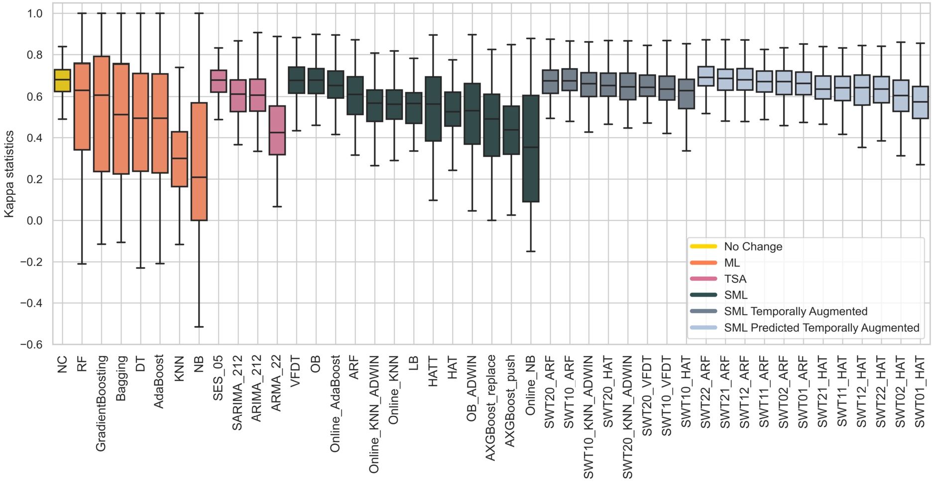
As SML methods, we test the Online Naïve Bayes, Online K-Nearest Neighbours, Online K-Nearest Neighbours with ADWIN, Very Fast Decision Tree (VFDT), Hoeffding Adaptive Tree (HAT), Extremely Fast Decision Tree (HATT), Adaptive Random Forest (ARF), Online Bagging (OB), Online Bagging with ADWIN (OBADWIN), Leveraging Bagging (LB), Online AdaBoost, and Adaptive XGBoost with both the push (AXGBoostpush) and the replace (AXGBoostreplace) strategy classifiers.
Lastly, we also apply two different temporal augmentations. In the first one, we add 1 or 2 past labels to the Online K-Nearest Neighbours with ADWIN (SWT10KNNADWIN, SWT20KNNADWIN), Very Fast Decision Tree (SWT10VFDT, SWT20VFDT), Hoeffding Adaptive Tree (SWT10HAT, SWT20HAT), and Adaptive Random Forest (SWT10ARF, SWT20ARF) classifiers. In the second one, we also add 1 or 2 past predicted label as recommended in [14], e.g. algorithms starting with SWT12 means that use 1 past label and 2 past predicted labels. We applied it to the Hoeffding Adaptive Tree (SWT01HAT, SWT11HAT, SWT21HAT, SWT02HAT, SWT12HAT, SWT22HAT), and Adaptive Random Forest (SWT01ARF, SWT11ARF, SWT21ARF, SWT02ARF, SWT12ARF, SWT22ARF) algorithms.
Figure 2 shows the box plot of the Kappa statistics results achieved by all the evaluated methods, grouped by types of algorithms (Baseline, ML, TSA, SML, SML Temporally Augmented, and SML Predicted Temporally Augmented). It is noteworthy that the No Change classifier, here used as the baseline, is one of the best approaches. Nevertheless, some methods have whiskers larger than the baseline, resulting in a high variability. This behaviour is highly evident for ML methods that obtain the best maxima and worst minima. It is also interesting that the Augmented SML algorithms outperform their respective base classifier. Notably, the methods augmented with the past predictions showed the best improvements, resulting in high mean and small interquartile ranges.
For this reason, for each group, in Fig. 3, we compared the value over time of the Kappa statistics of the best and worst algorithm w.r.t. the No Change classifier. Comparing the baseline with the TSA models, we notice that the Simple Exponential Smoothing algorithm (best TSA) performs similarly to the baseline, while the ARMA model (worst TSA) is much worse.
Fig. 3.
Kappa statistics results achieved over all the segments. The first column compares the best TSA, ML, SML, SML Temporally Augmented, and SML Predicted Temporally Augmented models w.r.t. the Baseline (No Change classifier), while the second column compares the worst TSA, ML, SML, SML Temporally Augmented, and SML Predicted Temporally Augmented models w.r.t. the Baseline.
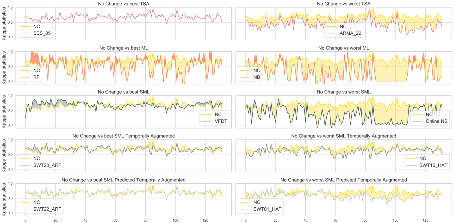
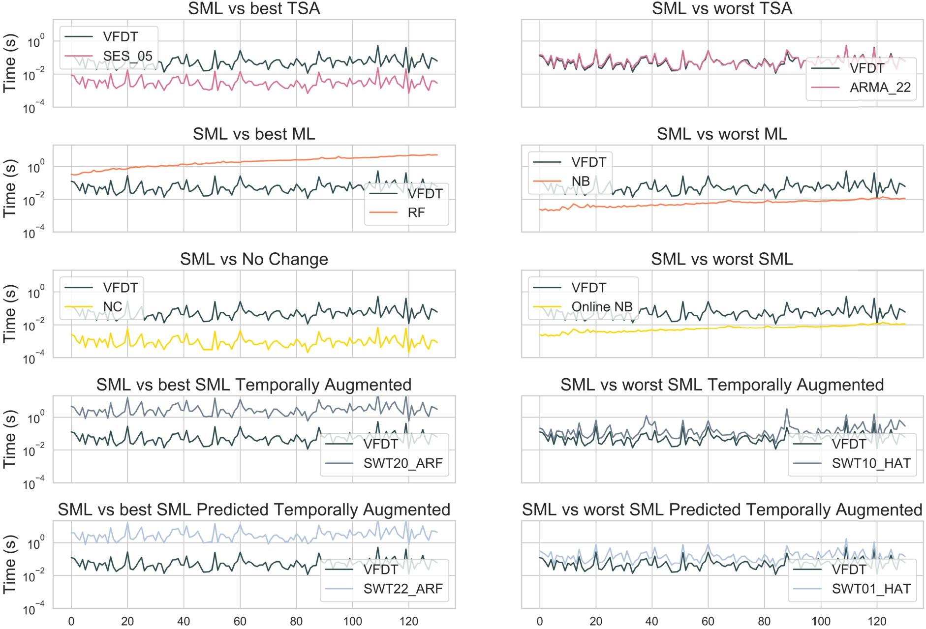
Fig. 4.
Time results achieved over all the segments. The first column compares the best TSA, ML, No Change, SML Temporally Augmented, and SML Predicted Temporally Augmented models w.r.t. the best SML model (VFDT classifier), while the second column compares the worst TSA, ML, SML, SML Temporally Augmented, and SML Predicted Temporally Augmented models w.r.t. the best SML model.
Undoubtedly, the label is insufficient for TSA methods, and it is necessary to consider the exogenous part of the data. For this purpose, there are the ML methods. In some segments, the Random Forest (best ML) model is better than the baseline, while the Naïve Bayes (worst ML) is almost always worse. Moreover, both models show high and low peaks, indicating a lack of stability. In fact, with datasets affected by continuous changes over time, as the one tested, there is the need to monitor the performance and, when they decrease, to retrain the model from scratch using more data.
We used SML models to avoid this problem, both with and without temporal augmentation. We can observe that, in some segments, the VFDT (best SML), SWT20ARF (best SML Temporally Augmented), and SWT22ARF (best SML Predicted Temporally Augmented) classifiers achieve better results than the baseline. They are more stable than ML models, as they can adapt independently to concept drifts. However, they are not still the best for the entire experiment. In conclusion, it is not enough to detect a concept drift, as SML does; there is a need to detect the changes in the temporal dependence over time, too. SML cannot do so since, once fixed, the number of temporal augmentations cannot be changed over time.
An essential requirement when analyzing algorithms for data streams is the execution time, which discriminates the models that use resources most efficiently. Figure 4 shows the execution time over the segments. It is worth noticing that as ML models accumulate data (the landmark window widens), the time and resources consumed increase. Instead, SML and TSA online models, being incremental approaches, consume constant time and resources, except for sporadic peaks due to “model adjustments” for adapting to changes. This analysis indicates that the right way to manage incoming data flows is one of the incremental models.
Fig. 5.
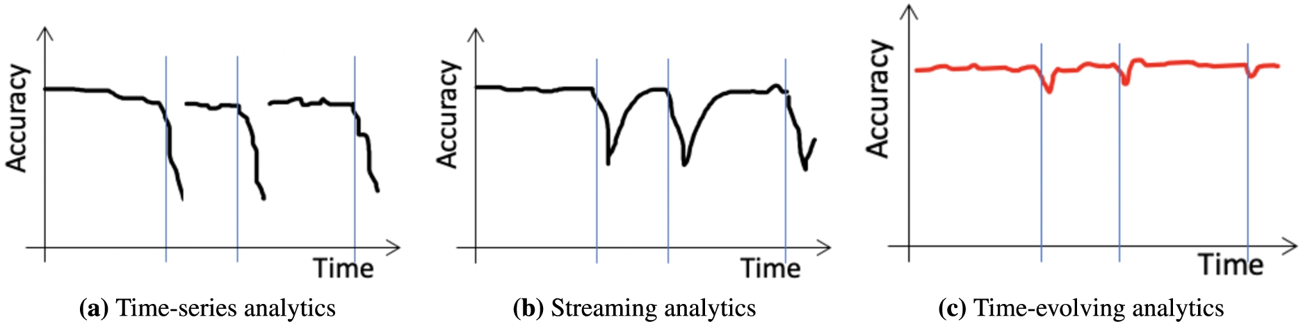
Type of analytics. Each vertical line represents a concept drift occurrence.
5.Challenges and benefits
We must address unique conceptual and technical challenges to succeed in this considerable potential. The first challenge is to identify a method to ignore past data when a change occurs while retaining the temporal dependence that still holds. TSA techniques offer solutions to measure auto-correlation [20]. Still, they assume that data points are identically distributed. Thus, practitioners periodically look for changes and refresh models accordingly (Fig. 5a). On the other way round, although SML offers a comprehensive collection of drift detectors [18,28] to adapt to new data when changes occur (Fig. 5b), a more sophisticated detector is required to monitor temporal dependence and selectively remember past data.
This leads to the following intriguing questions: given a data stream in which data points present temporal dependence and changes can occur at any time, can we continuously learn and adapt a model to keep it relevant? Would different types of changes (abrupt, gradual, and recurrent) make the problem harder or simpler? What would be the Markov-order impact on the model (i.e., the number of the past points to consider [34])? To what extent can we harness existing SML and TSA techniques for the task? What new methods are required? A second complementary challenge is incremental learning with novel stateful algorithms that process data points as they arrive and then discard them [2]. This challenge stems from the unbounded nature of data streams and the impossibility of storing them. We need to design single-pass [25] and low-time-complexity [31] algorithms analogously to what is done today in stream processing, where constant-time and polylog-space-complexity algorithms find a vast application [32]. Moreover, those models will need to explain why the predictions are correct and how much the users trust them. This is especially true for ambiguous situations where multiple possible future sequence outcomes are predicted.
A significant benefit of Time-Evolving Analytics would be continuously and fast adapting models to changes. The availability of predictive models in situations where historical data analytics fails to keep models relevant increases the potential for identifying new insights, taking the right decision, and acting in time. An added reason is the sequential nature of the models Time-Evolving Analytics would adaptively learn mining the short and long-lasting temporal dependence in the data streams (Fig. 5c). Practitioners would get a tool to explain fluctuations and predict the likelihood of possible alternative futures. Time-Evolving Analytics has the potential to simplify what-if analyses in selecting among complex alternatives in a volatile world. Last, developing stateful incremental algorithms that learn one sample at a time is very important. The smaller the data to process, the less sophisticated and the more scalable the tools are [31].
6.The envisioned framework
In time-series and data stream abstractions, the temporal aspect carries meaningful information; it thus requires a novel solution that redefines the theoretical guarantees to make learning from time-dependent data streams and evolving time series consistent.
6.1.Framework’s desiderata
Starting from TSA and SML’s cornerstones, our envisioned framework formalizes Time-Evolving Analytics’s foundations. Desiderata of the ideal framework include:
Problem agnostic (R1). This framework is not limited to a specific setting (e.g., only classification). Instead, it includes unsupervised and semi-supervised methodologies. These two domains are particularly favourable since many real-world data streams do not necessarily provide class labels, or when they do, labels may be late enough to jeopardize the model update.
No task boundaries (R6). Learning from the input data without requiring clear task divisions makes this framework applicable to never-ending data streams. Moreover, this large sample size enables determining the model from data with non-parametric approaches where the number and nature of the parameters can evolve.
Stateful learning (R5). Acknowledging data’s dynamic nature with its volume, variety, and velocity is at the framework’s core. In such a fast time-changing scenario, it is crucial to stateful detect patterns on the fly without storing all the data and passing through them multiple times. Ideally, models should efficiently handle a possible unlimited stream of high-dimensional ever-changing data (i.i.d., evolving, and not i.i.d. data streams) within bounded computational and memory resources while stateful learning from one data point at a time before discarding it.
Graceful forgetting (R4). Given the unbounded nature of data streams (i.i.d., evolving, and not i.i.d. data streams), graceful forgetting of trivial information is an important mechanism to balance stability and plasticity. Furthermore, it will be possible to revisit previously seen tasks to enhance the corresponding task knowledge by discarding useless information.
Selective remembering (R4). A further challenge is integrating new knowledge while preserving past information and retaining the temporal dependence that still holds (not i.i.d. data streams), aiming for a greater generalization over time. Forward transfer or zero-shot learning are essential concepts here, highlighting previously acquired knowledge to aid the learning of new tasks by increased data efficiency. The retained knowledge will also benefit from backward transfer, i.e., continue improving while learning future related tasks.
Adaptive learning (R4). The framework targets dynamic environments that may change unexpectedly. Methodologies must continuously adapt to the data distribution over time (evolving and not i.i.d. data streams). Adjusting to such concept drift represents a natural extension for their learning systems.
Learning sequences (R2). Real-world data streams (time-dependent time series, evolving and not i.i.d.) often contain dependence that spans multiple time steps and scales from seconds/minutes to months/years. Recognizing and predicting this dependence in the temporal sequences becomes essential to the model’s capability to make high-order predictions.66 Models should learn variable-order temporal sequences to correlate important patterns that happened many time steps in the past. Finally, an ideal algorithm should learn the order automatically and efficiently.
Forecasting alternatives (R3). The best prediction may not be sufficient in several situations. Indeed, there may be multiple possible future outcomes for a given temporal scenario. Therefore, algorithms should output a distribution of possible simultaneous future predictions and the associated confidence levels. The model can then evaluate the likelihood of each prediction online. In case of substantial uncertainty, the ability to simultaneously predict and assess each prediction’s probability becomes crucial.
6.2.A unifying model
No consensus exists on which statistical properties hold in a real-time scenario. Practitioners apply algorithms to data streams with unwarranted assumptions that could invalidate the results obtained. It is thus necessary to converge on a comprehensive Time-Evolving Analytics model. The framework must reassess the theoretical setting, formalize strategies for concept drift and temporal dependence, and conceive a unifying model incorporating temporal dependence.
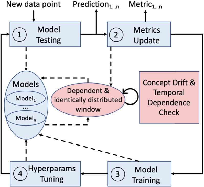
In literature, most drift detection methods use statistical tests that assume independent data. Temporal dependence often violates the assumptions of the statistical tests, incorrectly applying them and making irrelevant the detected changes [4,50]. There is a need to reassess the concept drift detection phase and the design decisions for change detectors. As for the former, it would be interesting to analyze the relationships between seasonality, trend, residual error, and concept drift. We should explore the relationship between concept drift detectors and anomaly detectors, which find rare points inconsistent with the distribution. Similarities between these areas are evident, and concepts such as zero-positive learning [26] can be crucial in the presence of rare events for both concept drift and temporal dependence. As for the latter, Fig. 6 shows a proposal for a new generation of change detectors that, in parallel to the concept drift detection, discover (i) if there is temporal dependence, (ii) how long this dependence is, and (iii) in case of temporal dependence changes when one stops, and another starts. Determining the number of lags in which a temporal dependence exists is crucial to adapt the model as in Change Point Detection methods [15]. An idea to explore is how to apply the Granger causality test [20] or the (Partial) AutoCorrelation functions incrementally – for example, using a window containing identically distributed and dependant data to train a model. When a new drift occurs or data into the window stops being temporal dependent, the window should slide, and the model should adapt consequently to it.
Fig. 6.
Proposed architecture to manage concept drift and temporal dependence.
6.3.A unifying methodology
More methodologies must be proposed to consider temporal dependence in the data stream while learning sequences to predict multiple alternative outcomes. The envisioned model alone is useless without the methodology necessary to use its algorithms. Such a methodology must include the capabilities for training and testing models (but without distinguishing the two tasks), choosing the best hyperparameter values and model components, and selecting the most appropriate metrics.
Prequential [17] and cross-validated prequential [7] evaluation approaches include a fading factor or a windowed evaluation to “forget” old predictions performance. This practice works well to handle the concept drift occurrences, but it is at risk with temporal dependence. Indeed, they consider short-term dependence but fail to consider long-term ones. The same type of window proposed in Fig. 6 may solve temporal dependence training and testing problems. Moreover, a new framework for evaluating analytics solutions for data streams is necessary [25]. In particular, new benchmark streams with several drifts of various types would ease the parallel training, testing, and comparison of different models. The starting point for the synthetic data generator is a set of Polya’s Urns [30]. Each urn contains a different number of black and white balls, depending on the colour. At each timestamp, the generator extracts a ball from one of the urns without replacing them. An empty urn gets refilled in the initial status unless a concept drift occurs. In this way, the generator creates sequences for which the exchangeability assumption holds, but the i.i.d. does not.
AutoML [23] is gaining popularity in the hyperparameter tuning scenario, but only a few autoML solutions are online in the literature [3,29,46]; none of them considers temporal dependence. A starting point might be autoML Lifelong ML challenge,77 to define a theoretical formalization that, taking into account i.i.d. and not i.i.d. data, allows to find the best model for a given scenario. The exploration shall not be limited to hyperparameters but should include choosing the continuous analysis pipeline’s best components. If successful, these methodologies will train in parallel and resource-wise efficient ways different versions of various models and use the window envisioned in Fig. 6 to continuously adapt the hyperparameter values to stay consistent with the concept drifts and temporal dependence.
The last point is about metrics selection. During the training phase, model validation is the only way to monitor the learning progress. Therefore, the correct selection of performance metrics is fundamental. On the one hand, it would be worth exploring the combination of the K-Temporal statistic [50] with the (cross-validated) prequential evaluation approach since the combination could give a valuable baseline metric to address not i.i.d. data. On the other hand, the window proposed in Fig. 6 may represent a suitable option for the (cross-validated) prequential evaluation approach combined with any chosen stand-alone metric. This combination could also give a valuable way to evaluate the model when the i.i.d. assumption does not hold. Moreover, we intend to identify new stand-alone metrics for monitoring if the model correctly considers temporal dependence during the learning phase. They are missing, and it is of fundamental importance to develop them.
7.Conclusions
We discussed several challenges that pertain online learning for time-evolving data streams, stressing the need for a unifying theory between Time-series Analytics and Streaming Machine Learning. These novel theoretical foundations will be a solid basis for forecasting multiple possible outcomes of a high-order sequence. Models learned with Time-Evolving Analytics will remain relevant even when changes like COVID-19 hit, allowing them to compete in volatile and uncertain markets.
We also discussed that the No Change detector can outperform the state-of-the-art ML/TSA/SML methods used in a classification streaming evaluation. Moreover, SML approaches with temporal augmentation represent only the first reasonable solution to incorporate the temporal aspect into the learning process. All these results strengthen our claim that when combined with concept drifts, the temporal dependence might significantly impact the learning process and evaluation. Thus temporal dependence should be considered during the learning process of the models. We hope that this paper will open several directions for future research. The lack of such a theory is the root cause of the current inability to adapt predictive models fast, continuously, and incrementally.
Notes
1 The term order refers to Markov order.
2 For instance, DeepMind claims to be able to forecast the next hour of rain using a deep generative model [35].
6 The term order refers to Markov order.
References
[1] | O. Anava, E. Hazan, S. Mannor and O. Shamir, Online learning for time series prediction, in: COLT, JMLR Workshop and Conference Proceedings, Vol. 30: , JMLR.org, (2013) , pp. 172–184, available at http://proceedings.mlr.press/v30/Anava13.html. |
[2] | B. Babcock, M. Datar, R. Motwani et al., Load shedding techniques for data stream systems, in: Proceedings of the 2003 Workshop on Management and Processing of Data Streams, Vol. 577: , Citeseer, (2003) , available at http://www-cs-students.stanford.edu/~datar/papers/mpds03.pdf. |
[3] | M. Bahri, B. Veloso, A. Bifet and J. Gama, AutoML for stream k-nearest neighbors classification, in: IEEE BigData, IEEE, (2020) , pp. 597–602. doi:10.1109/BigData50022.2020.9378396. |
[4] | A. Bifet, Classifier concept drift detection and the illusion of progress, in: ICAISC (2), LNCS, Vol. 10246: , Springer, (2017) , pp. 715–725. doi:10.1007/978-3-319-59060-8_64. |
[5] | A. Bifet and R. Gavaldà, Learning from time-changing data with adaptive windowing, in: Proceedings of the 2007 SIAM International Conference on Data Mining, SIAM, (2007) , pp. 443–448. doi:10.1137/1.9781611972771.42. |
[6] | A. Bifet, R. Gavaldà, G. Holmes and B. Pfahringer, Machine Learning for Data Streams with Practical Examples in MOA, MIT Press, (2018) . doi:10.7551/mitpress/10654.001.0001. |
[7] | A. Bifet, G.D.F. Morales, J. Read, G. Holmes and B. Pfahringer, Efficient online evaluation of big data stream classifiers, in: KDD, ACM, (2015) , pp. 59–68. doi:10.1145/2783258.2783372. |
[8] | A. Bifet, J. Read, I. Zliobaite, B. Pfahringer and G. Holmes, Pitfalls in benchmarking data stream classification and how to avoid them, in: ECML/PKDD (1), LNCS, Vol. 8188: , Springer, (2013) , pp. 465–479. doi:10.1007/978-3-642-40988-2_30. |
[9] | D.A. Bodenham and N.M. Adams, Continuous monitoring for changepoints in data streams using adaptive estimation, Stat. Comput. 27: (5) ((2017) ), 1257–1270. doi:10.1007/s11222-016-9684-8. |
[10] | G.E.P. Box and G.M. Jenkins, Time Series Analysis: Forecasting and Control, John Wiley & Sons, (2015) . ISBN 978-1-118-67502-1. |
[11] | L. de Carvalho Pagliosa and R.F. de Mello, Applying a kernel function on time-dependent data to provide supervised-learning guarantees, Expert Syst. Appl. 71: ((2017) ), 216–229. doi:10.1016/j.eswa.2016.11.028. |
[12] | M. De Lange, R. Aljundi, M. Masana, S. Parisot, X. Jia, A. Leonardis, G. Slabaugh and T. Tuytelaars, A continual learning survey: Defying forgetting in classification tasks, IEEE Transactions on Pattern Analysis and Machine Intelligence (2021). doi:10.1109/TPAMI.2021.3057446. |
[13] | L. Devroye, L. Györfi and G. Lugosi, A Probabilistic Theory of Pattern Recognition, Vol. 31: , Springer Science & Business Media, (1996) . doi:10.1007/978-1-4612-0711-5. |
[14] | T.G. Dietterich, Machine learning for sequential data: A review, in: SSPR/SPR, Lecture Notes in Computer Science, Vol. 2396: , Springer, (2002) , pp. 15–30. doi:10.1007/3-540-70659-3_2. |
[15] | Q. Duong, H. Ramampiaro and K. Nørvåg, Applying temporal dependence to detect changes in streaming data, Appl. Intell. 48: (12) ((2018) ), 4805–4823. doi:10.1007/s10489-018-1254-7. |
[16] | J. Gama, P. Medas, G. Castillo and P.P. Rodrigues, Learning with drift detection, in: SBIA, LNCS, Vol. 3171: , Springer, (2004) , pp. 286–295. doi:10.1007/978-3-540-28645-5_29. |
[17] | J. Gama, R. Sebastião and P.P. Rodrigues, On evaluating stream learning algorithms, Mach. Learn. 90: (3) ((2013) ), 317–346. doi:10.1007/s10994-012-5320-9. |
[18] | J. Gama, I. Zliobaite, A. Bifet, M. Pechenizkiy and A. Bouchachia, A survey on concept drift adaptation, ACM Comput. Surv. 46: (4) ((2014) ), 44:1–44:37. doi:10.1145/2523813. |
[19] | D. Giannone, L. Reichlin and D. Small, Nowcasting: The real-time informational content of macroeconomic data, Journal of Monetary Economics 55: (4) ((2008) ), 665–676. doi:10.1016/j.jmoneco.2008.05.010. |
[20] | C.W. Granger, Investigating causal relations by econometric models and cross-spectral methods, Econometrica: journal of the Econometric Society 37: (3) ((1969) ), 424–438. doi:10.2307/1912791. |
[21] | M. Harries and N.S. Wales, SPLICE-2 Comparative Evaluation: Electricity Pricing, (1999) , available at https://www.researchgate.net/publication/2562830_SPLICE-2_Comparative_Evaluation_Electricity_Pricing. |
[22] | W.D. Heaven, Our weird behavior during the pandemic is messing with AI models, MIT Technology Review (2020), available at https://www.technologyreview.com/2020/05/11/1001563/covid-pandemic-broken-ai-machine-learning-amazon-retail-fraud-humans-in-the-loop/. |
[23] | F. Hutter, L. Kotthoff and J. Vanschoren (eds), Automated Machine Learning – Methods, Systems, Challenges, The Springer Series on Challenges in Machine Learning, Springer, (2019) . doi:10.1007/978-3-030-05318-5. |
[24] | M.A. Johansson, A.M. Powers, N. Pesik, N.J. Cohen and J.E. Staples, Nowcasting the spread of Chikungunya virus in the Americas, PloS one 9: (8) ((2014) ), e104915. doi:10.1371/journal.pone.0104915. |
[25] | B. Krawczyk, L.L. Minku, J. Gama, J. Stefanowski and M. Wozniak, Ensemble learning for data stream analysis: A survey, Inf. Fusion 37: ((2017) ), 132–156. doi:10.1016/j.inffus.2017.02.004. |
[26] | T. Lee, J. Gottschlich, N. Tatbul, E. Metcalf and S. Zdonik, Greenhouse: A Zero-Positive Machine Learning System for Time-Series Anomaly Detection, 2018, CoRR, arXiv:1801.03168. |
[27] | C. Liu, S.C.H. Hoi, P. Zhao and J. Sun, Online ARIMA algorithms for time series prediction, in: AAAI, AAAI Press, (2016) , pp. 1867–1873, available at https://www.aaai.org/ocs/index.php/AAAI/AAAI16/paper/view/12135. |
[28] | J. Lu, A. Liu, F. Dong, F. Gu, J. Gama and G. Zhang, Learning under concept drift: A review, IEEE Trans. Knowl. Data Eng. 31: (12) ((2019) ), 2346–2363. doi:10.1109/TKDE.2018.2876857. |
[29] | J.G. Madrid, H.J. Escalante, E.F. Morales, W. Tu, Y. Yu, L. Sun-Hosoya, I. Guyon and M. Sebag, Towards AutoML in the presence of Drift: First results, 2019, CoRR, arXiv:1907.10772. |
[30] | H. Mahmoud, Pólya Urn Models, CRC Press, (2008) . doi:10.1201/9781420059847. |
[31] | A. McGregor, A. Pavan, S. Tirthapura and D.P. Woodruff, Space-efficient estimation of statistics over sub-sampled streams, Algorithmica 74: (2) ((2016) ), 787–811. doi:10.1007/s00453-015-9974-0. |
[32] | Z. Milosevic, W. Chen, A. Berry and F.A. Rabhi, Chapter 2 – real-time analytics, in: Big Data, R. Buyya, R.N. Calheiros and A.V. Dastjerdi, eds, Morgan Kaufmann, (2016) , pp. 39–61. doi:10.1016/C2015-0-04136-3. |
[33] | K. Panetta, Gartner Top 10 Data and Analytics Trends for 2021, 2021, 2022, available at: https://www.gartner.com/smarterwithgartner/gartner-top-10-data-and-analytics-trends-for-2021. |
[34] | L.R. Rabiner, A tutorial on hidden Markov models and selected applications in speech recognition, Proceedings of the IEEE 77: (2) ((1989) ), 257–286. doi:10.1109/5.18626. |
[35] | S. Ravuri, K. Lenc, M. Willson, D. Kangin, R. Lam, P. Mirowski, M. Fitzsimons, M. Athanassiadou, S. Kashem, S. Madge et al., Skilful precipitation nowcasting using deep generative models of radar, Nature 597: (7878) ((2021) ), 672–677. doi:10.1038/s41586-021-03854-z. |
[36] | J. Read, R.A. Rios, T. Nogueira and R.F. de Mello, Data streams are time series: Challenging assumptions, in: BRACIS (2), LNCS, Vol. 12320: , Springer, (2020) , pp. 529–543. doi:10.1007/978-3-030-61380-8_36. |
[37] | D. Reinsel, J. Gantz and J. Rydning, The digitization of the world from edge to core, Framingham: International Data Corporation 16 (2018), available at https://www.seagate.com/files/www-content/our-story/trends/files/idc-seagate-dataage-whitepaper.pdf. |
[38] | O. Russakovsky, J. Deng, H. Su, J. Krause, S. Satheesh, S. Ma, Z. Huang, A. Karpathy, A. Khosla, M. Bernstein et al., Imagenet large scale visual recognition challenge, International journal of computer vision 115: (3) ((2015) ), 211–252. doi:10.1007/s11263-015-0816-y. |
[39] | R.M. Sakia, The Box-Cox transformation technique: A review, Journal of the Royal Statistical Society: Series D (The Statistician) 41: (2) ((1992) ), 169–178. doi:10.2307/2348250. |
[40] | S. Shalev-Shwartz, Online learning and online convex optimization, Found. Trends Mach. Learn. 4: (2) ((2012) ), 107–194. doi:10.1561/2200000018. |
[41] | D. Silver, T. Hubert, J. Schrittwieser, I. Antonoglou, M. Lai, A. Guez, M. Lanctot, L. Sifre, D. Kumaran, T. Graepel et al., A general reinforcement learning algorithm that masters chess, shogi, and go through self-play, Science 362: (6419) ((2018) ), 1140–1144. doi:10.1126/science.aar6404. |
[42] | Y. Song, J. Lu, H. Lu and G. Zhang, Learning Data Streams With Changing Distributions and Temporal Dependency, IEEE Transactions on Neural Networks and Learning Systems (2021). doi:10.1109/TNNLS.2021.3122531. |
[43] | F. Takens, Detecting strange attractors in turbulence, in: Dynamical Systems and Turbulence, Warwick 1980, Springer, (1981) , pp. 366–381. doi:10.1007/BFb0091903. |
[44] | A. Tsymbal, The problem of concept drift: Definitions and related work, Computer Science Department, Trinity College Dublin 106: (2) ((2004) ), 58, available at https://www.scss.tcd.ie/publications/tech-reports/reports.04/TCD-CS-2004-15.pdf. |
[45] | V. Vapnik, The Nature of Statistical Learning Theory, Springer Science & Business Media, (2000) . doi:10.1007/978-1-4757-3264-1. |
[46] | J. Wilson, A.K. Meher, B.V. Bindu, S. Chaudhury, B. Lall, M. Sharma and V. Pareek, Automatically optimized gradient boosting trees for classifying large volume high cardinality data streams under concept drift, in: The NeurIPS’18 Competition, Springer, (2020) , pp. 317–335. doi:10.1007/978-3-030-29135-8_13. |
[47] | J.W. Wilson, N.A. Crook, C.K. Mueller, J. Sun and M. Dixon, Nowcasting thunderstorms: A status report, Bulletin of the American Meteorological Society 79: (10) ((1998) ), 2079–2100. doi:10.1175/1520-0477(1998)079<2079:NTASR>2.0.CO;2. |
[48] | J.T. Wu, K. Leung and G.M. Leung, Nowcasting and forecasting the potential domestic and international spread of the 2019-nCoV outbreak originating in Wuhan, China: A modelling study, The Lancet 395: (10225) ((2020) ), 689–697. doi:10.1016/S0140-6736(20)30260-9. |
[49] | J. Zhang, R. Verschae, S. Nobuhara and J.-F. Lalonde, Deep photovoltaic nowcasting, Solar Energy 176: ((2018) ), 267–276. doi:10.1016/j.solener.2018.10.024. |
[50] | I. Žliobaitė, A. Bifet, J. Read, B. Pfahringer and G. Holmes, Evaluation methods and decision theory for classification of streaming data with temporal dependence, Mach. Learn. 98: (3) ((2015) ), 455–482. doi:10.1007/s10994-014-5441-4. |
[51] | I. Žliobaitė, M. Pechenizkiy and J. Gama, An overview of concept drift applications, in: Big Data Analysis: New Algorithms for a New Society, (2016) , pp. 91–114. doi:10.1007/978-3-319-26989-4_4. |