Empirical evaluation of price-based technical patterns using probabilistic neural networks
Abstract
Technical analysis is the art of identifying patterns in historical data with the belief that certain patterns foretell future price movements. An empirical evaluation of the effectiveness of technical analysis is confounded by the subjectivity involved in identifying patterns. This work presents a robust framework for pattern identification using probabilistic neural networks (PNN). The thirty components of the Dow Jones Industrial Average and a set of ten indices are considered. Fourteen patterns are analyzed. In order to test the possibility that technical patterns are more predictable in certain market environments, the period under study (1990 – 2015) is partitioned into bull and bear markets and the statistical significance of profits earned by identified patterns observed in each environment is analyzed. A range of holding periods from 10 to 50 trading days is considered and a simple model of transaction costs is added. The study reveals that no pattern produces statistically and economically significant profits for a cross-section of stocks and indices analyzed, though a few patterns are more successful predictors. Bullish (bearish) patterns are more reliable predictors in bullish (bearish) market environments. These observations can be explained by the Adaptive Market Hypothesis with certain patterns becoming more accurate predictors in specific market environments.
Introduction
Technical analysis is the art of identifying geometric patterns in historical prices – often supplemented with volume-based signals – with the belief that occurrence of patterns are reliable predictors of price movement in the immediate future. Academic professionals and fundamental analysts typically scoff at technical analysis because of its paucity of quantitative justification. Recent works dealing with profitability of technical analysis based trading strategies have given some credence to the assertion that technical analysis may not be a complete farce. Brock et al. (1992) test the profitability of moving average rule (buying when shorter period moving average rises above longer period moving average, and selling when it falls below longer period moving average) and trading-range break out (buy when price rises above the observed local maximum and sell when it falls below the observed local minimum). They find statistically significant profits that cannot be explained using three null models of efficient market hypothesis – random walk, AR(1) and GARCH-M models. They observe further that volatility of returns following a buy signal is lower than volatility of returns following sell signal, thereby refuting the notion that higher returns for these strategies compensate higher inherent risks.
Osler and Chang (1995) test the profitability of head and shoulders pattern in foreign-exchange markets. They find the strategy yields economically significant profit in German Mark and Yen markets but not in other exchange rate markets studied in the work. They use a bootstrap method using random walk null model of efficient market hypothesis to conclude that returns from head and shoulders trading strategy are incompatible with the null hypothesis for German Mark and Yen exchange markets. Rejection of null model could either imply inefficiency of those exchange markets or the existence of a different null model compatible with efficient market hypothesis (for example, time varying mean). Other works Logue et al. (1978), Sweeney (1986), and Levich and Thomas (1993) also report statistically significant profits using technical analysis.
Savin et al. (2007) use pattern recognition method presented by Lo et al. (2000) to test if head-and-shoulders pattern has predictive power. After examining data for S&P 500 and Russell 2000 from 1990 to 1999, they conclude that the pattern has negligible predictive power when used as a stand-alone trading strategy, but has power to predict risk-adjusted excess returns over market portfolio returns. They conclude that the period studied in their work coincided with a bull market, and head-and-shoulders being a reversal pattern would not be a profitable stand-alone trading strategy.
Researchers have noted the failure of macro-economic models in explaining exchange rate volatility. Neely et al. (1997) and Stephan (2009) have assessed the effectiveness of technical patterns in explaining exchange rate fluctuations. Neely et al. (1997) apply genetic algorithm to study the profitability of technical patterns in foreign exchange markets. Genetic algorithm is used to design superior trading strategies based on filter rules and moving-average rules. The rule is tested in an out-of-sample period from 1981 – 1995 and found to generate statistically and economically significant profits. Neely et al. (1997) further show that the higher profits are not a compensation for bearing higher risks by examining betas. The significance of technical patterns in foreign exchange markets has been examined by Stephan (2006), Stephan (2008) and Stephan (2009). Stephan (2009) attributes the prevalence of technical analysis in foreign exchange markets to a virtuous circle whereby traders use it as a tool to form an expectation of current trends, in turn making technical analysis a more commonly used tool and increasing its effectiveness as a predictor. Neely et al. (2009) examine the time-varying effectiveness of technical patterns as predictors in foreign exchange market. They observe that filter-rules and moving-average technical rules produce statistically and economically significant profits from early 1970 to late 1980; however, by early 1990 such rules no longer produce statistically significant profits. They explain the observation as being consistent with Adaptive Market Hypothesis (Lo, 2004). Olson (2004) arrives at a similar conclusion, noting that moving-average trading rule profits (risk-adjusted) have declined from 3.5% during 1970 to around 0% from 1990 to 2000 across 18 exchange rate series. Chavarnakul and Enke (2008) employ generalized regression neural network (GRNN) to construct two trading strategies based on equivolume charting that predict the next day’s price using volume and price based technical indicators. They observe that using neural network improves the profitability of a moving average based trading rule in trending markets. However, the time period studied is rather limited - one year - and they only consider S&P 500 index. Furthermore, the difference in profitability between neural network based strategy and buy-and-hold strategy is not too large. Other works (Enke and Thawornwong 2005), (Li and Kuo 2008), (Leigh et al. 2005), (Chenoweth et al. 1996) have studied the application of neural networks in finance. Enke and Thawornwong (2005) test the hypothesis that neural networks can provide superior prediction of future returns based on their ability to identify non-linear relationships. They employ only fundamental measures and do not consider technical ones. Their neural network provides higher returns than buy-and-hold strategy, but they do not consider transaction costs. Scalar vector regression (SVR) has also been used in creating automated trading strategies: (Hong et al. 2010; Huang 2012; Kazema et al. 2013; Wang and Pardalos 2014).
A challenging aspect for any work attempting to perform an empirical assessment of technical analysis based trading strategies is the automated identification of technical pattern. Osler and Chang (1995) employ a method based on peaks and troughs. They define a peak as a local maximum of closing price that is at least χ percent higher than the preceding trough and a trough as a local minimum at least χ percent lower than the preceding peak. χ is selected based on standard deviation; in their work they select a set of values for the cutoff parameter χ. Lo et al. (2000) use a novel method based on kernel smoothing. They use a Gaussian kernel in smoothing, with a constant smoothing parameter chosen by visual inspection of smoothed price curve. Approach used by Lo et al. (2000), and Osler and Chang (1995) has the shortcoming of using a constant smoothing parameter over the entire price history. Heteroskedasticity in stock prices is a well documented phenomenon (Bollerslev, 1987). Lo et al. (2000) acknowledge this shortcoming. Methods employed by Osler and Chang (1995) and Lo et al.(2000) use sequence of successive local maximum and minimum to identify patterns. In addition, they use a number of tests to make sure there is close fidelity to the technical patterns they recognize, for example, Lo et al. (2000) require the tops in a double-top pattern to be within 1.5% of their mean. It is conceivable for a double-top pattern to occur with successive tops being slightly more than 1.5% of their average. Further, it is distinctly possible that a different smoothing in an area may reveal part of a pattern. An approach that insists on observing local extrema in a specific order while using a constant smoothing parameter is likely to miss such pattern occurrences.
This work applies neural networks for recognizing technical patterns in stock prices and evaluates the performance of patterns as predictors of future price movements. Neural networks are uniquely suited to the task of character recognition, and pattern recognition has distinct similarities to character recognition (Beymer and Poggio 1996). A class of neural networks called probabilistic neural networks or PNN is employed. PNN were introduced by Specht (1990). The process of constructing a PNN is simpler than that required for a back-propagation neural network. PNN is used to identify the following patterns: ascending-triangle, descending-triangle, head-and-shoulders, cup-and-handle, double-top, double-bottom, triple-top, triple-bottom, broadening-top, down-price-channel, rising-wedge, falling-wedge, up-symmetric-triangle, down-symmetric-triangle and down-price-channel for ten indices and for the thirty components of Dow Jones Industrial Average. To evaluate the empirical performance of a trading strategy based on each of the patterns, 15 years of history for indices (from 2000 to 2015) and 25 years of history for Dow Jones components (from 1990 to 2015) is considered.
Technical analysts also resort to the use of volume-based indictors as confirming signals during pattern formation phase. However, there is little agreement between technical analysts on the exact definition of confirming signals. The confirming signals rarely constitute the defining aspect of the pattern. To illustrate this point, consider the definition of head-and-shoulders pattern from two sources Investopedia (2016) and Wikipedia (2016). While Investopedia (2016) mentions nothing about the role of volume, Wikipedia (2016) qualifies its description of the pattern using volume: “The left shoulder is formed at the end of an extensive move during which volume is noticeably high.”. However, Wikipedia (2016) further qualifies the role of volume in left shoulder by mentioning that the breakout below neckline in that region may occur on high or low volume. “The drawn neckline of the pattern represents a support level, and assumption cannot be taken that the Head and Shoulder formation is completed unless it is broken and such breakthrough may happen to be on more volume or may not be”. Because volume does not seem to play the defining role in pattern definition and there is some disagreement on the exact definition of the volume-based confirming signal, this work does not consider volume for the purpose of pattern identification.
The remainder of this paper is organized as follows: Section 3 describes the algorithm used in identifying the patterns, Section 4 describes the probabilistic neural network used, Section 5 discusses the application of the probabilistic neural network in identifying the patterns for ten indices and thirty Dow Jones components. Section 6 concludes the work.
2Algorithm for identification of technical patterns
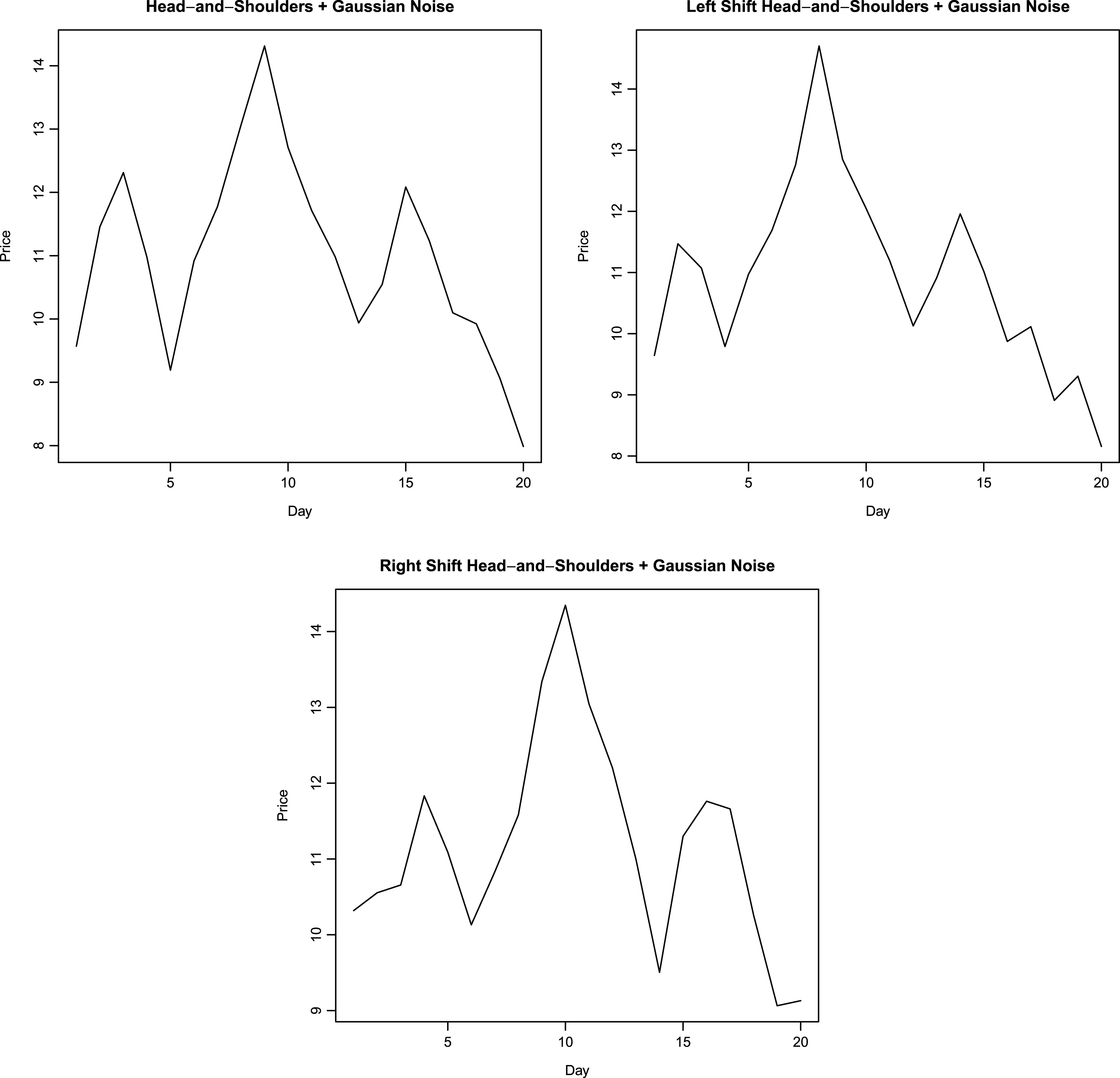
To recognize a pattern using neural networks, a representation of the pattern is required that is robust to local noise. As a first step, prototypes of price patterns are first created manually. The prototypes are very geometric, with prices rising and falling along straight lines. Figures 1–3 show the manually generated prototypes on a plot. These prototypes are referred as prototype patterns in this work. All prototype patterns are twenty days in length. Next, Gaussian noise is added to each day’s price in prototype pattern. The standard deviation of noise is selected to be smaller than the maximum daily price change in the prototype plots. In the present work, standard deviation of added noise is taken to be 0.3. 200 realizations of random variable are obtained at each point, thereby yielding 200 perturbed plots corresponding to each prototype pattern. An example of perturbed plot for head-and-shoulders pattern is shown in Fig. 4. Next, each point in the unperturbed price plot is moved to the left by one day. First and last points corresponding to the first and last day are kept at their original positions. The third days price displaces the second day’s price and so on. 200 realizations of Gaussian noise with mean = 0 and variance = 0.09 are added to each day’s price yielding 200 new perturbed plots. An example of left-shift perturbed plot for head-and-shoulders pattern is shown in Fig. 4. In a similar manner to the left-shift, right shift is performed on unperturbed base price pattern, keeping the first and last day’s prices at their original location. After right-shifting by one day, 200 realizations of Gaussian noise are added to each day’s price yielding another 200 perturbed plots. Gaussian noise has mean = 0 and variance = 0.09. An example of right-shift perturbed plot for head-and-shoulders pattern is shown in Fig. 4. This procedure produces 601 examples of price patterns corresponding to each technical pattern under consideration. These 601 plots (six hundred perturbed plots and one prototype plot) corresponding to each pattern comprise the training set for the probabilistic neural network. PNN are simpler to construct as compared with multi-layer back-propagation neural networks. For example, back-propagation neural network implementation in R package neuralnet (Fritsch et al. 2012) fails to converge for the data set in this work (14 × 601 plots). Increasing the number of hidden neurons or the maximum iterations does not help to overcome the problem of non-convergence during training. Also, increasing the number of hidden layers or hidden neurons increases the time taken by back-propagation neural network during learning. This demonstrates the attractive feature of network simplicity for a PNN. Details regarding construction of PNN are presented in Section 4.
Fig.1
Manually generated pattern shapes.
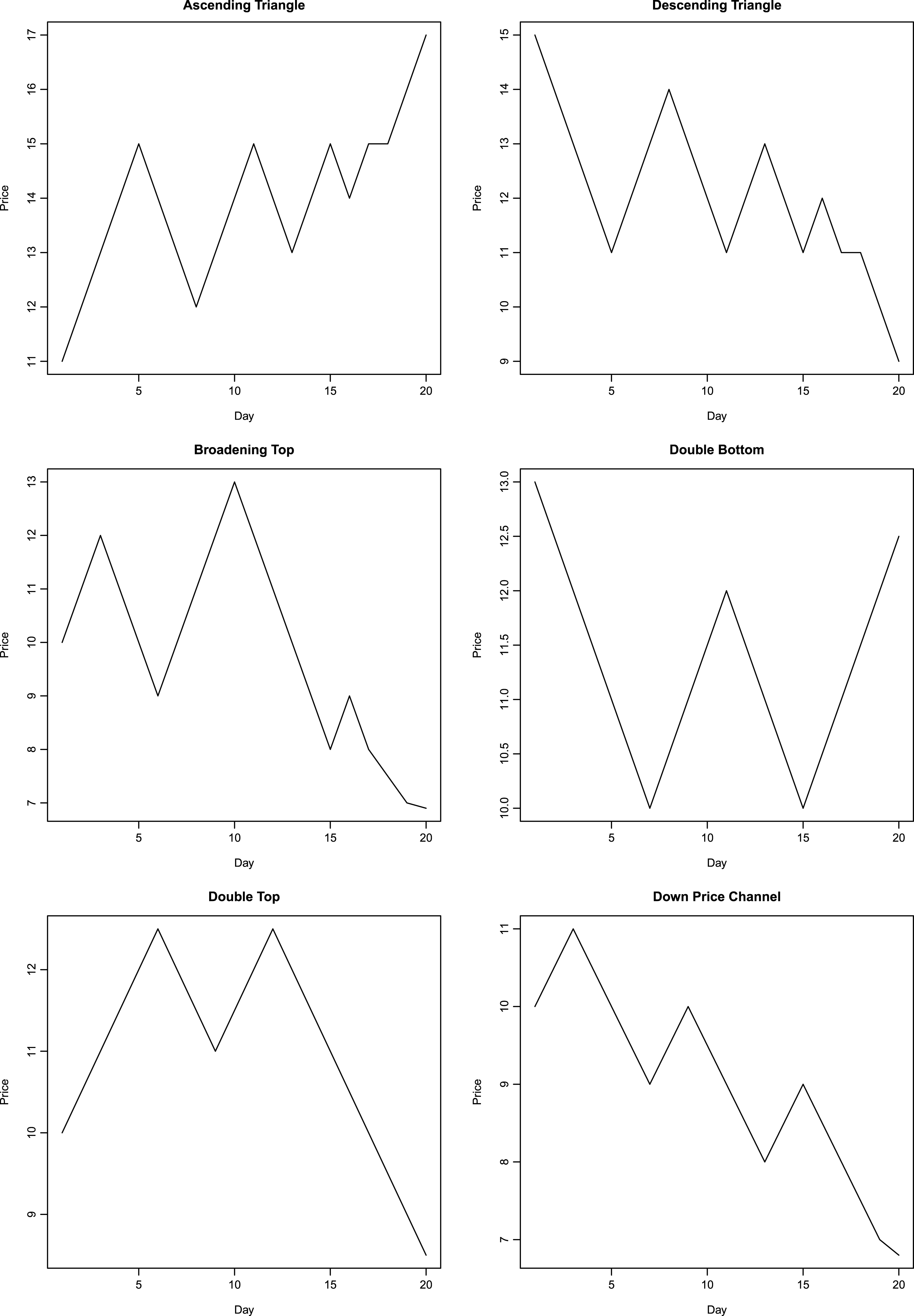
Fig.2
Manually generated pattern shapes.
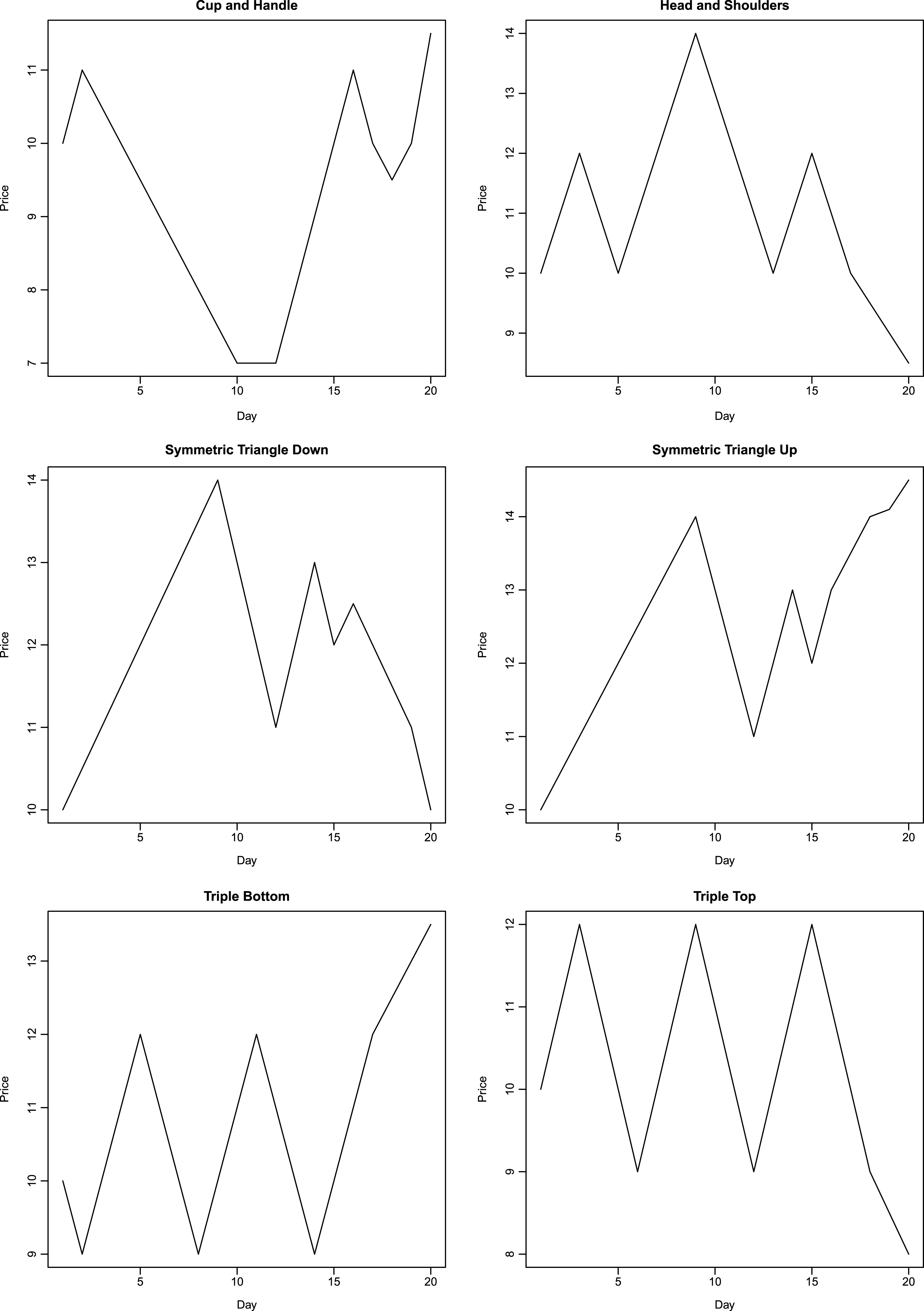
Fig.3
Manually generated pattern shapes.
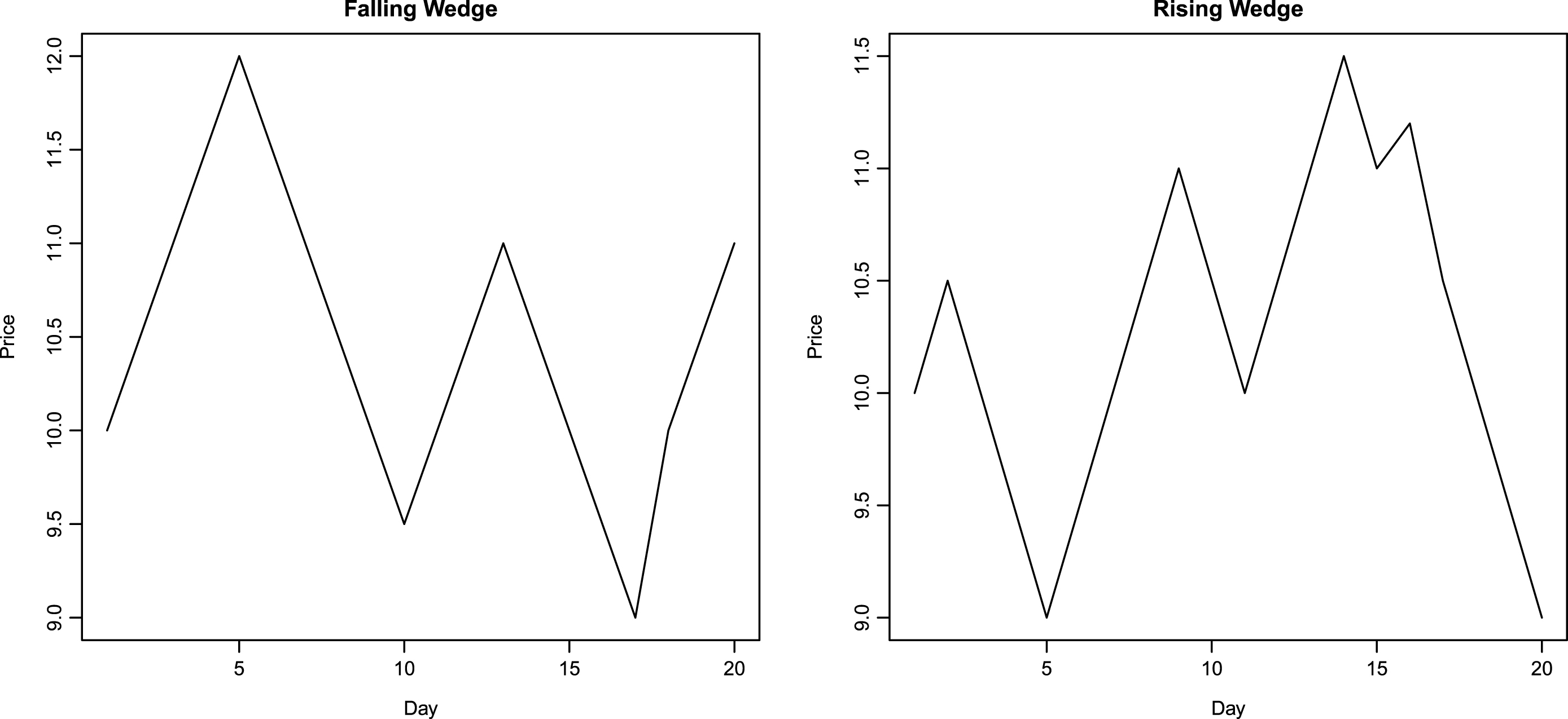
Fig.4
Perturbed head-and-shoulders pattern with left and right shift.
In order to classify a pattern into one of several classes under consideration, or to determine that it does not belong to any of the classes, a representation of pattern is required. This representation is akin to a fingerprint: patterns belonging to one class should produce similar representations. This task is similar to the task confronted in character recognition where a handwritten character must be matched to one of several known characters. However, unlike in character recognition where a character must belong to one of several classes (alphabets), one also needs to discriminate the case where a pattern does not match any of the classes. To that end, the algorithm for pattern recognition presented in this work can also be used for character recognition.
The prototype patterns and their perturbations are constructed to have the same length, i.e. they have same number of days. This is true of all patterns considered. In this work, the prototype patterns are chosen to be 20 days in length. This requirement does not impose any restriction on the length of patterns that can be classified using this algorithm. Further, because window sizes considered are greater than or equal to 20 days, resizing the series down to a length of 20 days does not introduce significant interpolation inaccuracy. The prices are normalized. Let pmin denote the minimum price, p the daily price and pmax the maximum price observed over the twenty day length of a pattern. Normalized prices are calculated using equation (1).
(1)
pn=p-pminpmax-pminThis set of twenty normalized prices is the fingerprint of the pattern. The perturbations of a pattern will have fingerprints that are closer to the fingerprints of prototype (unperturbed) pattern. Distance is defined as Euclidean distance in the twenty-dimensional space. More formally, distance between two patterns is given by equation (2). xi and yi are the normalized prices.
(2)
distance=√∑20i=1(xi-yi)2A probabilistic neural network (PNN) is constructed to classify patterns belonging to the types considered in this work. Details of constructing the network are presented in the next section. In order to identify a pattern, a range of window lengths varying from twenty days to sixty days are considered. Let l denote the window length, L denote the price series length and i denote an index in price series. For each window length, the algorithm checks price pattern between i and i + l days, where index i ranges from the beginning of price series to L - l - 1 (inclusive range). The price list observed between days [i, i + l] is scaled to a new price list with 20 elements; the scaled price list now has the same length as the prototype patterns. The price series length scaling is performed using equation (3). Rescaling is analogous to resizing the price series length to 20 days. Price for day j in actual price series becomes the price on day dj in rescaled price series where dj is given by equation (3). Price for days between dj and dj+1 are interpolated.
(3)
dj=⌊j-il×20⌋j∈[i,i+l]Fingerprint of each rescaled price series is calculated as a tuple of twenty normalized prices using Equation (1). This fingerprint is presented as input to PNN for classification. In order to identify the case where a pattern does not match any of the types considered in this work, the PNN uses a threshold. Details are presented in the next section.
3Details on probabilistic neural network
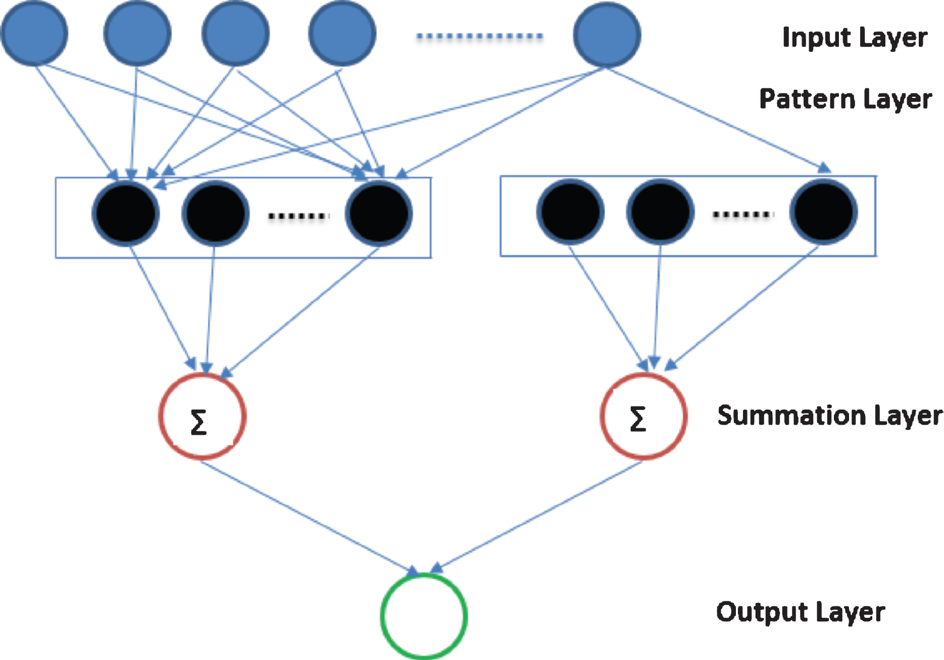
Probabilistic neural networks were first introduced by Specht (1990) as a four-layer neural network capable of representing non-linear decision boundaries for a classification problem and offering significant speedup as compared to the training time of a back-propagation multi-layer feed-forward neural network. Prababilistic neural networks have four layers: input layer, pattern layer, summation layer and output layer. The first layer is the input layer. The number of input units is equal to the dimensionality of the problem. In this work, a pattern is represented by a set of twenty normalized prices, hence the first layer of PNN is comprised of twenty input units. The input units transmit their input as output, without applying any other transformation. The second layer of the PNN, known as pattern layer, is defined by the training set data. In this work, the training data consists of 14 × 601 inputs – each pattern type has 600 perturbations and one base price series, giving 601 training data points for each pattern type, and there are fourteen patterns types examined. The second layer therefore consists of 14 × 601 units. Units in second layer of a PNN network are grouped into classes the PNN network is meant to classify. In this work, second layer units are grouped into fourteen groups. Each group consists of 601 units. Each unit applies a Gaussian activation function to its input. If the input is denoted as x, output generated by m unit in second layer pattern j is given by equation (4). xm denotes the normalized price vector corresponding to mth training input. xm and x are vectors of size 20.
(4)
ym,j=1(√2π|Σ|)D×exp(-(x-xm)Σ-1(x-xm)T2)D=20m=1,2,…601xm={xm,1,xm,2,…xm,20}x={x1,x2,…x20}In Equation (4), xi refers to the training data point corresponding to i pattern unit. It is the normalized price. σ is the variance-covariance matrix defined on training data belonging to a pattern type. It is calculated as shown in Equation (5). There are fourteen variance covariance matrices used in the PNN network, one corresponding to each pattern type.
(5)
Σi,j=∑601k=1(xi,k-¯xi)(xj,k-¯xj)¯xi=∑601k=1xi,k601¯xj=∑601k=1xj,k601i∈[1,20]j∈[1,20]The third layer of a PNN is the summation layer. Summation layer sums up the output from second layer’s units belonging to a group. There are fourteen summation layer units in this work, each producing an output corresponding to the likelihood of the data matching a pattern type. Input for a summation layer unit is the set of outputs generated by second layer units belonging to a particular group. Summation layer unit’s output is shown in equation (6). m denotes the index of pattern type, there are 14 types of pattern considered in this work.
(6)
zm=∑601j=1ym,jm∈1,2,…14The fourth layer of a PNN is the output layer, it picks the group having the maximum value and classifies the data as belonging to that group. The fourth layer has one unit, its output is given in Equation (7).
(7)
Final Output=m ∃ zm>zi ∀m≠iA PNN always classifies a data into one of the classes. In order to identify the case where a data set does not match any pattern, this work requires the maximum output to be greater than 100 times the output from other groups. Let zm denote the maximum output from third layer and zi denote an output from another unit in third layer. m denotes the third layer unit having maximum output and i is another third-layer unit. For the data to be classified as matching pattern m, this work requires that Equation (8) hold for all i ≠ m.
(8)
zmzi≥100 ∀m≠iThe threshold value of 100 is an empirical parameter, higher values of threshold will produce very close matches to the pattern while rejecting potential matches that do not comport with the threshold. Low values of threshold parameter will produce greater number of matches while producing an occasional false positive by identifying a data to match a pattern when it does not (i.e. a technical analyst would disagree with the classification).
A diagrammatic representation of the probabilistic neural network is shown in Fig. 5.
Fig.5
Representation of PNN.
4Application of pattern recognition in empirical analysis
This work attempts to identify technical patterns enumerated earlier in prices of thirty Dow Jones components and in ten indices: S&P 500 index and nine Russell indices (Table 1). For Dow Jones components and S&P 500 index, price history from 1990 to 2015 is analyzed. For Russell indices, price history from 2000 to 2015 is studied because prices for these indices are available from 2000 onwards. Patterns with length ranging from 20 trading days to 40 trading days are considered (40 trading days is around two months). Manifestations of patterns with longer duration are not identified. This restriction reflects a compromise between reducing computation time and considering a window length that covers common occurrences of patterns. Bulkowski (2005, p. 805) observes average length of falling-wedge pattern to be less than two months, average length of flag pattern to be less than two weeks (Bulkowski 2005, p. 903), average length of broadening tops and bottoms to be two months (Bulkowski 2005, p. 81), average length between left and right shoulder tops of head-and-shoulders pattern to be two months (Bulkowski 2005, p. 415) and average length of an island pattern to be just over a month (Bulkowski 2005, p. 491). According to Bulkowski (2005, p. 143), pattern length can vary depending on bull or bear market. A range of holding periods (10, 20, 30, 40 and 50 trading days) is considered in order to test the possibility that some patterns may need longer holding periods for price to move in accordance with the pattern’s prediction.
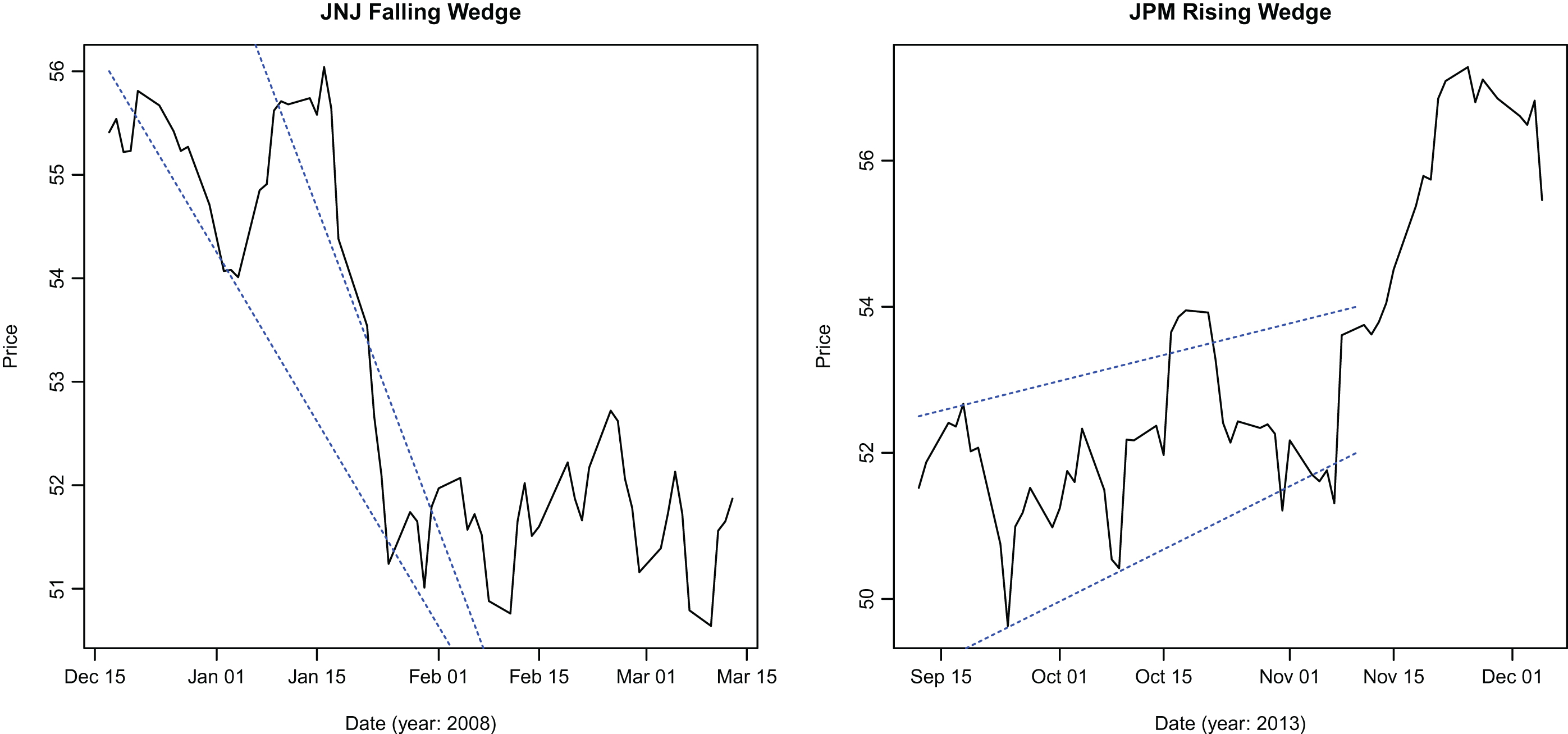
On each day, the PNN based pattern identification algorithm is applied to price series of 30 Dow components and 10 indices to see if a pattern can be identified over the window length. Dividend and split adjusted closing prices for the 30 Dow components and 10 indices are used. After identification, the pattern is validated using an independent test (described below). Once a pattern is identified and validated, its return is recorded over the holding period. Return is calculated as pi+N-pipi, where N is the holding period length. In order to examine the possibility that technical patterns may be more effective predictors in certain market environments, the period from 1990 to 2015 is partitioned into bull or bear markets depending upon the market performance (S&P 500 index) during the period. The periods were selected using publicized dates for the onset of bull and bear markets widely reported in media. This selection entails some in-sample bias because the partitions are selected ex-post, though the bias is alleviated to a certain extent by the relatively long duration of periods selected compared to the length of patterns and holding periods considered. A study conducted for the entire period yields similar qualitative results. Since the patterns are either bullish or bearish in their predictions, it is appropriate to partition the period between bullish or bearish markets and test the predictive power of all patterns in the two market environments. The classification is shown in Table 2. Returns observed for different patterns are tabulated in tables presented. Examples of identified patterns are presented in Figures 6, 7 and 8.
Table 1
Indices analyzed
| Ticker | Index Name |
| SPY | S&P 500 |
| IWM | Russell 2000 |
| IWB | Russell 1000 |
| IWR | Russell Midcap |
| IWC | Russell Microcap |
| XLG | Russell Top 50 |
| IWF | Russell 1000 Growth |
| IWD | Russell 1000 Value |
| IWO | Russell 2000 Growth |
| IWN | Russell 2000 Value |
Table 2
Partition by market trend
| Begin Date | End Date | Classification |
| 1991-01-01 | 1999-01-01 | Bull Market |
| 2002-01-01 | 2003-04-01 | Bear Market |
| 2003-03-01 | 2007-09-01 | Bull Market |
| 2007-10-01 | 2009-02-01 | Bear Market |
| 2009-03-01 | 2015-01-01 | Bull Market |
Fig.6
Specimen patterns identified by the algorithm.
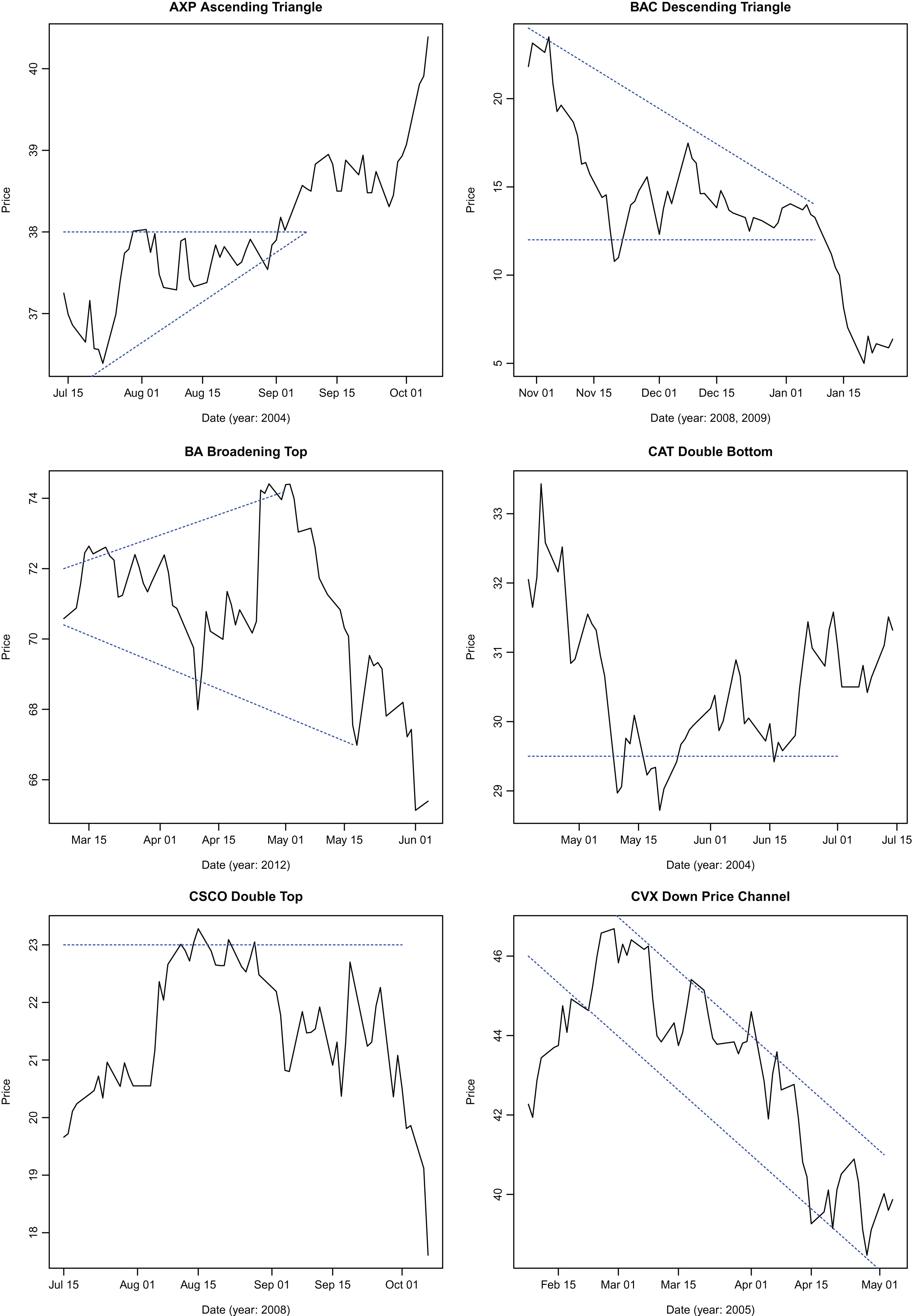
Fig.7
Specimen patterns identified by the algorithm.
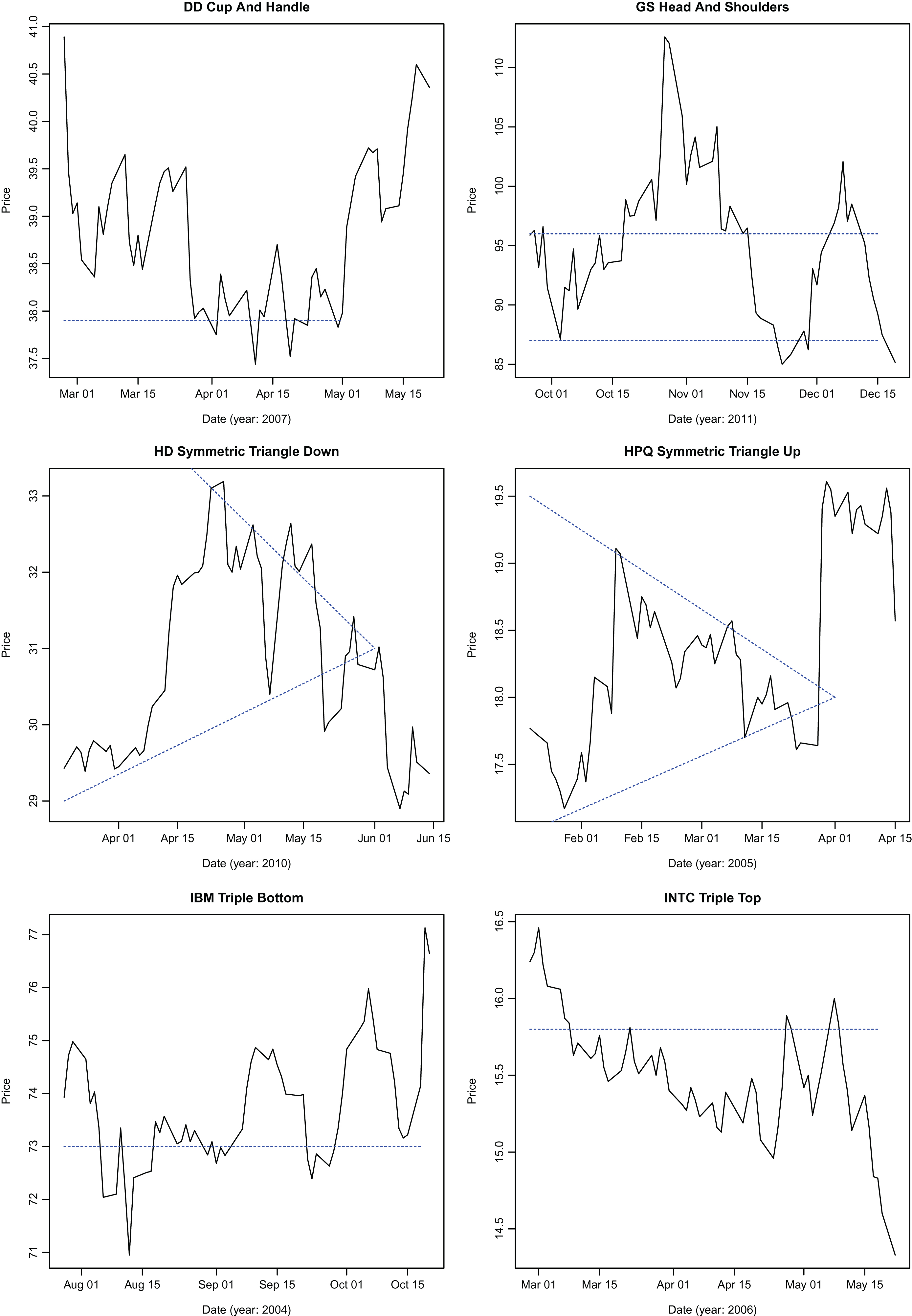
Fig.8
Specimen patterns identified by the algorithm.
Bullish and bearish environments are selected to coincide with changes in S&P 500 index over a period of a year or more, marked by well publicized market events (Table 2). Shorter periods – less than a year – were not used in order to reduce in-sample bias because the partitions are being selected ex-post. The period from 1990 – 1999 is marked by a steady rise in markets, without any major market black-swan event like Black Monday (crash of 1987) or technology crash. 2002 – 2003 partition is widely recognized as the period of technology bubble burst. 2003 – 2007 partition is recognized as the bull market spawned by brisk growth of mortgage lending; 2007 – 2009 partition is the ensuing period now referred as the Great Recession and 2009 – 2015 is the period of recovery from the Great Recession.
In order to validate identified patterns, a price-based test is added. The validation test is based on observing a set of high and low prices in a certain order. A technical pattern is characterized as an ordered set of high and low prices attained during the pattern’s observation period. Lo et al. (2000) have used kernel smoothing techniques to identify local price maxima and minima. Locally weighted scatter-plot smoothing algorithm (LOESS) with a quadratic polynomial employed for local fitting is used for price smoothing. Smoothed daily prices are compared to their neighboring prices to identify local extrema (maximum or minimum) by comparing the closing price for a day with the closing price of preceding and following trading days. If the closing price is higher than its neighbors, the price is a local maximum. Likewise, if it is lower than its neighbors, it is a local minimum. The identified pattern must have an occurrence of high-low price sequence characterizing the pattern. If an identified pattern fails the validation test, it is rejected. The high-low sequence for the patterns is shown in Table 4. Parameters employed in locally weighted scatterplot smoothing algorithm are tabulated in 3.
Table 3
Parameters used in LOESS smoothing
| Parameter | Value |
| Smoothing | 2 |
| Polynomial Degree | |
| Span | 0.4 |
| Kernel | Gaussian (Least |
| Squares Fitting) |
Table 4
Validating identified patterns
| Pattern | High-Low Order |
| Ascending Triangle | (H,L,H,L,H) |
| Descending Triangle | (L,H,L,H,L) |
| Broadening Top | (H,L,H,L,H,L) |
| Double Bottom | (L,H,L) |
| Double Top | (H,L,H) |
| Down Price Channel | (H,L,H,L,H,L) |
| Cup and Handle | (H,L,H,L,H) |
| Head and Shoulders | (H,L,H,L,H,L) |
| Symmetric Triangle Down | (H,L,H,L,H) |
| Symmetric Triangle Up | (H,L,H,L,H) |
| Triple Bottom | (L,H,L,H,L) |
| Triple Top | (H,L,H,L,H) |
| Falling Wedge | (H,L,H,L,H,L) |
| Rising Wedge | (H,L,H,L,H,L) |
Recognized and validated patterns are not manually evaluated to ensure correct classification. Technical analysts employ additional tests for classifying a price series as a technical pattern. To the extent that those validation tests are not employed, certain price series may have been misclassified.
Trading strategies based on technical patterns are often associated with trading rules. Trading rules are diverse, ranging from simple price increase or decrease based decisions to complex conditions involving volume. In order to study the impact of trading rules on the ability of technical patterns to forecast future price movements, a simple trading rule is applied: following the identification of the pattern, closing price is observed after three days. If the close price has not moved in accordance with the prediction of the technical pattern, no trading is done for that pattern instance. As an example, let i denote the day on which a technical pattern is recognized. Closing price is observed for i + 3 day and compared with closing price for i day. If the price change is not in accord with the bullish or bearish price prediction of the pattern, no trading is done for that pattern occurrence. Holding period begins from i + 4 day and ends on i + 13 day (both days inclusive) to ensure there is no in-sample bias. Three-day period is an empirical parameter; it is meant to test the accuracy of technical patterns as a price predictor. Increasing this period can increase the reliability of patterns at the expense of foregoing trading for more days following pattern identification.
Figures 6, 7 and 8 demonstrate the effectiveness of the algorithm in identifying patterns.
After a technical pattern is identified by the algorithm, price change is recorded for one unit of asset for the duration of the holding period. In order to ensure that there is no in-sample bias, holding period begins after pattern identification, validation and application of trading rule. A range of holding periods – 10, 20, 30, 40 and 50 trading-days – are considered. Technical analysis categorizes the technical patterns as bullish or bearish – bullish patterns are supposed to presage bullish price movement and bearish patterns are harbingers of future price declines. Table 5 shows this classification. In order to assess the statistical significance of profits for the trading strategy based on respective technical patterns, a one-sided t-test is performed. One-sided test is appropriate to test the bullish or bearish characterization of the patterns. 95% significance threshold is used; thestatistically significant patterns observed during bull and bear markets are reported in Tables 6 and 7 for Dow Jones components and in Tables 8 and 9 for indices respectively. Other patterns were not statistically significant. Null hypothesis for the test is that the technical patterns have no predictive power for future price movements.
Table 5
Bullish or bearish classification of technical patterns
| Pattern | Bullish or Bearish Predictor |
| Ascending Triangle | Bullish |
| Descending Triangle | Bearish |
| Broadening Top | Bearish |
| Double Bottom | Bullish |
| Double Top | Bearish |
| Down Price Channel | Bearish |
| Cup and Handle | Bullish |
| Head and Shoulders | Bearish |
| Symmetric Triangle Down | Bearish |
| Symmetric Triangle Up | Bullish |
| Triple Bottom | Bullish |
| Triple Top | Bearish |
| Wedge Falling | Bullish |
| Wedge Rising | Bearish |
Table 6
Statistically significant patterns observed during bull markets for dow components
| Asset | Holding | Pattern | Obs. | t-Stat | P | Mean |
| Period | Value | |||||
| AXP | 30 | Double Bottom | 13 | 2.263 | 0.021 | 0.977 |
| AXP | 30 | Cup and Handle | 5 | 2.045 | 0.048 | 2.385 |
| AXP | 40 | Cup and Handle | 5 | 2.222 | 0.038 | 1.560 |
| AXP | 40 | Falling Wedge | 52 | 1.801 | 0.039 | 0.771 |
| AXP | 50 | Double Bottom | 13 | 2.680 | 0.009 | 1.703 |
| AXP | 50 | Falling Wedge | 52 | 2.393 | 0.010 | 1.280 |
| BAC | 30 | Falling Wedge | 42 | 1.812 | 0.039 | 0.343 |
| BAC | 40 | Double Bottom | 20 | 2.442 | 0.012 | 0.711 |
| BAC | 40 | Symmetric Triangle Up | 35 | 2.013 | 0.026 | 0.361 |
| BAC | 40 | Falling Wedge | 42 | 1.764 | 0.042 | 0.420 |
| BAC | 50 | Symmetric Triangle Up | 35 | 1.957 | 0.029 | 0.418 |
| BAC | 50 | Falling Wedge | 42 | 2.209 | 0.016 | 0.628 |
| BA | 10 | Falling Wedge | 50 | 1.848 | 0.035 | 0.481 |
| BA | 20 | Falling Wedge | 50 | 2.588 | 0.006 | 1.102 |
| BA | 30 | Falling Wedge | 50 | 2.213 | 0.016 | 0.996 |
| BA | 40 | Falling Wedge | 50 | 2.914 | 0.003 | 1.451 |
| BA | 50 | Falling Wedge | 50 | 3.652 | 0.000 | 2.319 |
| CAT | 20 | Falling Wedge | 35 | 2.453 | 0.010 | 1.342 |
| CAT | 30 | Double Bottom | 20 | 1.855 | 0.039 | 1.928 |
| CAT | 30 | Falling Wedge | 35 | 2.326 | 0.013 | 1.576 |
| CAT | 50 | Triple Bottom | 10 | 2.424 | 0.018 | 2.158 |
| CAT | 50 | Falling Wedge | 35 | 3.336 | 0.001 | 3.009 |
| CSCO | 20 | Double Bottom | 17 | 1.770 | 0.047 | 0.458 |
| CSCO | 20 | Falling Wedge | 51 | 2.388 | 0.010 | 0.272 |
| CSCO | 40 | Double Bottom | 17 | 1.902 | 0.037 | 0.628 |
| CSCO | 50 | Falling Wedge | 51 | 2.101 | 0.020 | 0.455 |
| CVX | 10 | Falling Wedge | 45 | 1.958 | 0.028 | 0.487 |
| CVX | 40 | Symmetric Triangle Up | 39 | 2.094 | 0.021 | 1.120 |
| DD | 10 | Double Bottom | 29 | 2.316 | 0.014 | 0.478 |
| DD | 10 | Falling Wedge | 46 | 1.682 | 0.050 | 0.270 |
| DD | 20 | Falling Wedge | 46 | 1.795 | 0.040 | 0.437 |
| DD | 30 | Falling Wedge | 46 | 2.686 | 0.005 | 0.785 |
| DD | 40 | Falling Wedge | 46 | 4.225 | 0.000 | 1.339 |
| DD | 50 | Symmetric Triangle Up | 29 | 1.775 | 0.043 | 0.671 |
| DD | 50 | Falling Wedge | 46 | 3.775 | 0.000 | 1.312 |
| DIS | 10 | Double Bottom | 15 | 2.025 | 0.031 | 0.511 |
| DIS | 20 | Falling Wedge | 43 | 2.528 | 0.008 | 0.666 |
| DIS | 30 | Double Bottom | 15 | 1.768 | 0.049 | 0.756 |
| DIS | 30 | Falling Wedge | 43 | 3.804 | 0.000 | 1.069 |
| DIS | 40 | Double Bottom | 15 | 2.915 | 0.005 | 1.425 |
| DIS | 40 | Falling Wedge | 43 | 4.093 | 0.000 | 1.276 |
| DIS | 50 | Double Bottom | 15 | 3.238 | 0.003 | 1.421 |
| DIS | 50 | Symmetric Triangle Up | 24 | 2.435 | 0.011 | 1.399 |
| DIS | 50 | Triple Bottom | 18 | 2.104 | 0.025 | 1.010 |
| DIS | 50 | Falling Wedge | 43 | 4.209 | 0.000 | 1.627 |
| GE | 20 | Triple Bottom | 10 | 3.054 | 0.006 | 0.523 |
| GE | 20 | Falling Wedge | 49 | 1.929 | 0.030 | 0.255 |
| GE | 30 | Triple Bottom | 10 | 2.786 | 0.010 | 0.825 |
| GE | 40 | Double Bottom | 19 | 2.239 | 0.019 | 0.601 |
| GE | 40 | Triple Bottom | 10 | 2.092 | 0.031 | 0.878 |
| GE | 40 | Falling Wedge | 49 | 2.281 | 0.013 | 0.283 |
| GE | 50 | Double Bottom | 19 | 1.745 | 0.049 | 0.464 |
| GE | 50 | Triple Bottom | 10 | 2.388 | 0.019 | 0.816 |
| GE | 50 | Falling Wedge | 49 | 2.969 | 0.002 | 0.490 |
| HD | 10 | Double Bottom | 18 | 2.277 | 0.018 | 0.571 |
| HD | 10 | Symmetric Triangle Up | 39 | 2.254 | 0.015 | 0.320 |
| HD | 20 | Double Bottom | 18 | 3.497 | 0.001 | 1.225 |
| HD | 20 | Symmetric Triangle Up | 39 | 2.804 | 0.004 | 0.651 |
| HD | 30 | Double Bottom | 18 | 2.647 | 0.008 | 1.336 |
| HD | 30 | Symmetric Triangle Up | 39 | 2.185 | 0.017 | 0.743 |
| HD | 30 | Falling Wedge | 46 | 2.044 | 0.023 | 0.687 |
| HD | 40 | Double Bottom | 18 | 3.284 | 0.002 | 1.813 |
| HD | 40 | Symmetric Triangle Up | 39 | 3.045 | 0.002 | 1.047 |
| HD | 40 | Falling Wedge | 46 | 2.284 | 0.014 | 0.925 |
| HD | 50 | Double Bottom | 18 | 3.038 | 0.004 | 1.858 |
| HD | 50 | Symmetric Triangle Up | 39 | 3.303 | 0.001 | 1.376 |
| HD | 50 | Falling Wedge | 46 | 2.969 | 0.002 | 1.306 |
| HPQ | 30 | Triple Bottom | 16 | 2.460 | 0.013 | 0.431 |
| HPQ | 40 | Triple Bottom | 16 | 2.267 | 0.019 | 0.464 |
| IBM | 20 | Falling Wedge | 49 | 3.170 | 0.001 | 1.657 |
| IBM | 30 | Falling Wedge | 49 | 3.048 | 0.002 | 1.871 |
| IBM | 40 | Triple Bottom | 15 | 2.229 | 0.021 | 2.791 |
| IBM | 40 | Falling Wedge | 49 | 3.066 | 0.002 | 2.193 |
| IBM | 50 | Triple Bottom | 15 | 2.086 | 0.027 | 2.698 |
| IBM | 50 | Falling Wedge | 49 | 2.297 | 0.013 | 2.570 |
| INTC | 20 | Double Bottom | 22 | 2.609 | 0.008 | 0.764 |
| INTC | 30 | Double Bottom | 22 | 3.049 | 0.003 | 0.912 |
| INTC | 40 | Double Bottom | 22 | 2.595 | 0.008 | 1.166 |
| INTC | 40 | Symmetric Triangle Up | 28 | 2.062 | 0.024 | 0.537 |
| INTC | 50 | Symmetric Triangle Up | 28 | 2.012 | 0.027 | 0.635 |
| INTC | 50 | Falling Wedge | 38 | 1.712 | 0.048 | 0.479 |
| JNJ | 10 | Symmetric Triangle Up | 33 | 2.249 | 0.016 | 0.320 |
| JNJ | 20 | Symmetric Triangle Up | 33 | 1.787 | 0.042 | 0.399 |
| JNJ | 20 | Falling Wedge | 59 | 2.094 | 0.020 | 0.463 |
| JNJ | 30 | Symmetric Triangle Up | 33 | 2.303 | 0.014 | 0.823 |
| JNJ | 30 | Falling Wedge | 59 | 2.385 | 0.010 | 0.744 |
| JNJ | 40 | Double Bottom | 20 | 1.900 | 0.036 | 0.856 |
| JNJ | 40 | Symmetric Triangle Up | 33 | 3.792 | 0.000 | 1.311 |
| JNJ | 40 | Falling Wedge | 59 | 2.540 | 0.007 | 0.764 |
| JNJ | 50 | Double Bottom | 20 | 2.366 | 0.014 | 1.210 |
| JNJ | 50 | Symmetric Triangle Up | 33 | 2.974 | 0.003 | 1.538 |
| JNJ | 50 | Falling Wedge | 59 | 3.059 | 0.002 | 0.922 |
| JPM | 20 | Symmetric Triangle Up | 35 | 2.204 | 0.017 | 0.692 |
| JPM | 30 | Symmetric Triangle Up | 35 | 2.899 | 0.003 | 1.117 |
| JPM | 40 | Symmetric Triangle Up | 35 | 2.361 | 0.012 | 1.079 |
| JPM | 50 | Cup and Handle | 5 | 2.485 | 0.028 | 0.900 |
| KO | 20 | Double Bottom | 18 | 1.941 | 0.034 | 0.285 |
| KO | 20 | Falling Wedge | 40 | 2.254 | 0.015 | 0.378 |
| KO | 30 | Falling Wedge | 40 | 2.186 | 0.017 | 0.389 |
| KO | 40 | Double Bottom | 18 | 2.109 | 0.025 | 0.508 |
| KO | 40 | Falling Wedge | 40 | 2.085 | 0.022 | 0.428 |
| KO | 50 | Falling Wedge | 40 | 2.953 | 0.003 | 0.608 |
| MCD | 10 | Double Bottom | 17 | 2.568 | 0.010 | 0.631 |
| MCD | 20 | Double Bottom | 17 | 2.161 | 0.023 | 0.785 |
| MCD | 30 | Double Bottom | 17 | 2.101 | 0.025 | 1.038 |
| MCD | 30 | Symmetric Triangle Up | 29 | 2.867 | 0.004 | 0.939 |
| MCD | 40 | Symmetric Triangle Up | 29 | 1.808 | 0.040 | 0.680 |
| MCD | 40 | Falling Wedge | 51 | 2.530 | 0.007 | 0.845 |
| MCD | 50 | Falling Wedge | 51 | 3.324 | 0.001 | 1.286 |
| MMM | 20 | Falling Wedge | 35 | 2.304 | 0.014 | 1.105 |
| MMM | 40 | Symmetric Triangle Up | 29 | 2.262 | 0.016 | 1.424 |
| MMM | 40 | Falling Wedge | 35 | 2.679 | 0.006 | 1.844 |
| MMM | 50 | Falling Wedge | 35 | 3.235 | 0.001 | 2.686 |
| MRK | 10 | Falling Wedge | 47 | 1.772 | 0.041 | 0.198 |
| MRK | 20 | Symmetric Triangle Up | 31 | 1.800 | 0.041 | 0.395 |
| MRK | 20 | Falling Wedge | 47 | 2.247 | 0.015 | 0.539 |
| MRK | 40 | Falling Wedge | 47 | 2.022 | 0.024 | 0.722 |
| MRK | 50 | Symmetric Triangle Up | 31 | 2.705 | 0.005 | 0.772 |
| MRK | 50 | Falling Wedge | 47 | 1.925 | 0.030 | 0.700 |
| MSFT | 10 | Triple Bottom | 14 | 2.065 | 0.029 | 0.299 |
| MSFT | 20 | Triple Bottom | 14 | 2.975 | 0.005 | 0.546 |
| MSFT | 30 | Symmetric Triangle Up | 35 | 1.717 | 0.047 | 0.448 |
| MSFT | 30 | Triple Bottom | 14 | 2.115 | 0.026 | 0.713 |
| MSFT | 40 | Triple Bottom | 14 | 2.165 | 0.024 | 0.541 |
| MSFT | 40 | Falling Wedge | 42 | 2.049 | 0.023 | 0.514 |
| MSFT | 50 | Symmetric Triangle Up | 35 | 2.166 | 0.019 | 0.790 |
| MSFT | 50 | Triple Bottom | 14 | 2.196 | 0.023 | 0.668 |
| MSFT | 50 | Falling Wedge | 42 | 2.329 | 0.012 | 0.696 |
| PFE | 10 | Triple Bottom | 11 | 2.296 | 0.021 | 0.361 |
| PFE | 20 | Double Bottom | 20 | 2.754 | 0.006 | 0.414 |
| PFE | 40 | Symmetric Triangle Up | 34 | 1.853 | 0.036 | 0.321 |
| PFE | 50 | Double Bottom | 20 | 1.795 | 0.044 | 0.563 |
| PFE | 50 | Symmetric Triangle Up | 34 | 1.778 | 0.042 | 0.409 |
| PG | 10 | Symmetric Triangle Up | 28 | 3.024 | 0.003 | 0.316 |
| PG | 20 | Symmetric Triangle Up | 28 | 3.406 | 0.001 | 0.549 |
| PG | 20 | Falling Wedge | 52 | 2.924 | 0.003 | 0.747 |
| PG | 30 | Double Bottom | 17 | 1.917 | 0.036 | 0.601 |
| PG | 30 | Symmetric Triangle Up | 28 | 3.500 | 0.001 | 0.496 |
| PG | 30 | Falling Wedge | 52 | 3.665 | 0.000 | 1.068 |
| PG | 40 | Double Bottom | 17 | 3.551 | 0.001 | 1.100 |
| PG | 40 | Symmetric Triangle Up | 28 | 2.482 | 0.010 | 0.705 |
| PG | 40 | Falling Wedge | 52 | 3.392 | 0.001 | 1.107 |
| PG | 50 | Double Bottom | 17 | 3.382 | 0.002 | 1.689 |
| PG | 50 | Symmetric Triangle Up | 28 | 2.100 | 0.022 | 0.680 |
| PG | 50 | Falling Wedge | 52 | 4.687 | 0.000 | 1.414 |
| TRV | 40 | Double Bottom | 15 | 2.531 | 0.012 | 1.112 |
| TRV | 40 | Falling Wedge | 49 | 1.798 | 0.039 | 0.781 |
| TRV | 50 | Double Bottom | 15 | 2.747 | 0.007 | 1.656 |
| TRV | 50 | Symmetric Triangle Up | 28 | 1.735 | 0.047 | 0.952 |
| TRV | 50 | Falling Wedge | 49 | 2.029 | 0.024 | 1.006 |
| T | 10 | Falling Wedge | 43 | 2.102 | 0.021 | 0.158 |
| T | 20 | Falling Wedge | 43 | 2.290 | 0.013 | 0.259 |
| T | 30 | Falling Wedge | 43 | 2.505 | 0.008 | 0.331 |
| T | 40 | Triple Bottom | 13 | 1.794 | 0.048 | 0.436 |
| T | 40 | Falling Wedge | 43 | 4.291 | 0.000 | 0.689 |
| T | 50 | Double Bottom | 16 | 1.845 | 0.042 | 0.366 |
| T | 50 | Triple Bottom | 13 | 1.928 | 0.038 | 0.525 |
| T | 50 | Falling Wedge | 43 | 3.790 | 0.000 | 0.735 |
| UTX | 10 | Falling Wedge | 40 | 1.724 | 0.046 | 0.339 |
| UTX | 20 | Double Bottom | 20 | 1.896 | 0.036 | 0.873 |
| UTX | 30 | Double Bottom | 20 | 2.319 | 0.016 | 1.274 |
| UTX | 30 | Symmetric Triangle Up | 34 | 2.864 | 0.004 | 1.017 |
| UTX | 30 | Falling Wedge | 40 | 1.686 | 0.050 | 0.920 |
| UTX | 40 | Double Bottom | 20 | 3.040 | 0.003 | 1.523 |
| UTX | 40 | Symmetric Triangle Up | 34 | 2.614 | 0.007 | 1.111 |
| UTX | 40 | Falling Wedge | 40 | 1.906 | 0.032 | 1.214 |
| UTX | 50 | Double Bottom | 20 | 3.624 | 0.001 | 2.149 |
| UTX | 50 | Symmetric Triangle Up | 34 | 2.236 | 0.016 | 1.340 |
| UTX | 50 | Falling Wedge | 40 | 2.508 | 0.008 | 1.644 |
| VZ | 40 | Falling Wedge | 53 | 2.486 | 0.008 | 0.467 |
| VZ | 50 | Falling Wedge | 53 | 2.530 | 0.007 | 0.610 |
| WMT | 10 | Falling Wedge | 48 | 1.812 | 0.038 | 0.310 |
| WMT | 40 | Double Bottom | 26 | 2.889 | 0.004 | 1.310 |
| WMT | 40 | Falling Wedge | 48 | 1.831 | 0.037 | 0.877 |
| WMT | 50 | Double Bottom | 26 | 2.539 | 0.009 | 1.288 |
| WMT | 50 | Falling Wedge | 48 | 1.911 | 0.031 | 0.839 |
| XOM | 10 | Falling Wedge | 42 | 2.814 | 0.004 | 0.575 |
| XOM | 20 | Falling Wedge | 42 | 1.693 | 0.049 | 0.363 |
| XOM | 40 | Double Bottom | 18 | 2.005 | 0.030 | 1.489 |
| XOM | 40 | Symmetric Triangle Up | 25 | 2.053 | 0.025 | 1.041 |
| XOM | 50 | Double Bottom | 18 | 2.656 | 0.008 | 2.210 |
| XOM | 50 | Symmetric Triangle Up | 25 | 1.842 | 0.039 | 1.164 |
Table 7
Statistically Significant Patterns Observed During Bear Markets for Dow Components
| Asset | Holding | Pattern | Obs. | T-Stat | P | Mean |
| Period | Value | |||||
| BAC | 50 | Rising Wedge | 10 | -2.425 | 0.018 | -3.166 |
| BA | 30 | Rising Wedge | 8 | -2.262 | 0.027 | -5.180 |
| BA | 40 | Rising Wedge | 8 | -2.867 | 0.010 | -5.926 |
| BA | 50 | Rising Wedge | 8 | -3.196 | 0.006 | -6.711 |
| GE | 20 | Rising Wedge | 6 | -2.204 | 0.035 | -0.906 |
| GE | 50 | Down Price Channel | 7 | -2.730 | 0.015 | -1.570 |
| HPQ | 50 | Rising Wedge | 8 | -2.117 | 0.034 | -1.166 |
| INTC | 30 | Rising Wedge | 9 | -2.247 | 0.026 | -1.541 |
| INTC | 40 | Rising Wedge | 9 | -2.517 | 0.016 | -2.191 |
| JPM | 30 | Rising Wedge | 8 | -1.928 | 0.045 | -1.879 |
| JPM | 50 | Rising Wedge | 8 | -2.117 | 0.034 | -2.381 |
| KO | 40 | Rising Wedge | 6 | -2.316 | 0.030 | -0.777 |
| MRK | 20 | Rising Wedge | 8 | -1.900 | 0.047 | -1.974 |
| MRK | 40 | Rising Wedge | 8 | -2.250 | 0.027 | -2.827 |
| MRK | 50 | Rising Wedge | 8 | -2.139 | 0.032 | -3.067 |
| MSFT | 30 | Rising Wedge | 7 | -2.480 | 0.021 | -1.513 |
| MSFT | 40 | Rising Wedge | 7 | -3.968 | 0.003 | -2.128 |
| MSFT | 50 | Rising Wedge | 7 | -3.805 | 0.003 | -2.117 |
| PFE | 20 | Rising Wedge | 9 | -2.319 | 0.023 | -0.582 |
| PFE | 30 | Rising Wedge | 9 | -2.628 | 0.014 | -0.967 |
| PFE | 40 | Rising Wedge | 9 | -2.698 | 0.012 | -1.008 |
| PFE | 50 | Rising Wedge | 9 | -2.795 | 0.010 | -1.052 |
| TRV | 40 | Rising Wedge | 7 | -2.747 | 0.014 | -2.831 |
| TRV | 50 | Rising Wedge | 7 | -2.284 | 0.028 | -1.913 |
| T | 40 | Rising Wedge | 8 | -2.585 | 0.016 | -1.678 |
| T | 50 | Rising Wedge | 8 | -4.724 | 0.001 | -2.360 |
| UTX | 20 | Rising Wedge | 7 | -1.914 | 0.049 | -2.831 |
| UTX | 50 | Rising Wedge | 7 | -1.914 | 0.049 | -3.962 |
| XOM | 10 | Rising Wedge | 9 | -2.175 | 0.029 | -0.990 |
| XOM | 20 | Rising Wedge | 9 | -3.046 | 0.007 | -1.578 |
| XOM | 30 | Rising Wedge | 9 | -2.893 | 0.009 | -1.901 |
| XOM | 40 | Rising Wedge | 9 | -2.223 | 0.027 | -2.021 |
| XOM | 50 | Rising Wedge | 9 | -2.631 | 0.014 | -3.120 |
Table 8
Statistically significant patterns observed during bull markets for indices
| Asset | Holding | Pattern | Obs. | T-Stat | P | Mean |
| Period | Value | |||||
| IWB | 10 | Cup and Handle | 7 | 7.703 | 0.000 | 1.131 |
| IWB | 10 | Symmetric Triangle Up | 53 | 2.045 | 0.023 | 0.308 |
| IWB | 20 | Cup and Handle | 7 | 3.877 | 0.003 | 1.873 |
| IWB | 20 | Symmetric Triangle Up | 53 | 4.720 | 0.000 | 0.901 |
| IWB | 20 | Falling Wedge | 62 | 2.527 | 0.007 | 0.649 |
| IWB | 30 | Symmetric Triangle Up | 53 | 3.743 | 0.000 | 1.181 |
| IWB | 30 | Falling Wedge | 62 | 2.126 | 0.019 | 0.865 |
| IWB | 40 | Cup and Handle | 7 | 2.523 | 0.020 | 2.402 |
| IWB | 40 | Symmetric Triangle Up | 53 | 3.083 | 0.002 | 1.264 |
| IWB | 40 | Falling Wedge | 62 | 3.165 | 0.001 | 1.345 |
| IWB | 50 | Symmetric Triangle Up | 53 | 3.687 | 0.000 | 1.590 |
| IWB | 50 | Falling Wedge | 62 | 3.146 | 0.001 | 1.589 |
| IWC | 10 | Double Bottom | 10 | 1.922 | 0.042 | 0.329 |
| IWC | 20 | Cup and Handle | 5 | 2.637 | 0.023 | 1.413 |
| IWC | 30 | Double Bottom | 10 | 2.693 | 0.011 | 1.583 |
| IWD | 10 | Cup and Handle | 9 | 2.018 | 0.037 | 0.494 |
| IWD | 10 | Triple Bottom | 7 | 2.697 | 0.015 | 0.674 |
| IWD | 20 | Cup and Handle | 9 | 3.841 | 0.002 | 1.405 |
| IWD | 20 | Symmetric Triangle Up | 57 | 3.021 | 0.002 | 0.518 |
| IWD | 20 | Falling Wedge | 69 | 2.906 | 0.002 | 0.937 |
| IWD | 30 | Cup and Handle | 9 | 6.663 | 0.000 | 2.035 |
| IWD | 30 | Symmetric Triangle Up | 57 | 3.779 | 0.000 | 0.898 |
| IWD | 30 | Falling Wedge | 69 | 2.156 | 0.017 | 0.833 |
| IWD | 40 | Cup and Handle | 9 | 7.449 | 0.000 | 2.682 |
| IWD | 40 | Symmetric Triangle Up | 57 | 3.961 | 0.000 | 1.042 |
| IWD | 40 | Falling Wedge | 69 | 2.044 | 0.022 | 1.020 |
| IWD | 50 | Cup and Handle | 9 | 8.812 | 0.000 | 3.456 |
| IWD | 50 | Symmetric Triangle Up | 57 | 3.478 | 0.000 | 1.199 |
| IWD | 50 | Triple Bottom | 7 | 4.316 | 0.002 | 1.602 |
| IWD | 50 | Falling Wedge | 69 | 3.046 | 0.002 | 1.335 |
| IWF | 10 | Falling Wedge | 50 | 1.745 | 0.044 | 0.207 |
| IWF | 20 | Falling Wedge | 50 | 1.704 | 0.047 | 0.429 |
| IWF | 30 | Triple Bottom | 22 | 2.035 | 0.027 | 0.664 |
| IWF | 40 | Triple Bottom | 22 | 3.295 | 0.002 | 1.255 |
| IWF | 50 | Triple Bottom | 21 | 5.870 | 0.000 | 1.973 |
| IWM | 20 | Falling Wedge | 77 | 2.054 | 0.022 | 0.725 |
| IWM | 30 | Double Bottom | 27 | 1.715 | 0.049 | 1.271 |
| IWM | 40 | Double Bottom | 27 | 2.535 | 0.009 | 1.397 |
| IWM | 40 | Symmetric Triangle Up | 46 | 2.238 | 0.015 | 0.983 |
| IWM | 40 | Falling Wedge | 76 | 3.992 | 0.000 | 1.813 |
| IWM | 50 | Falling Wedge | 76 | 3.473 | 0.000 | 1.729 |
| IWN | 10 | Cup and Handle | 11 | 2.011 | 0.035 | 1.092 |
| IWN | 10 | Triple Bottom | 18 | 3.379 | 0.002 | 0.620 |
| IWN | 20 | Cup and Handle | 11 | 4.993 | 0.000 | 2.220 |
| IWN | 20 | Symmetric Triangle Up | 36 | 1.693 | 0.050 | 0.593 |
| IWN | 20 | Triple Bottom | 18 | 2.816 | 0.006 | 0.874 |
| IWN | 30 | Cup and Handle | 11 | 2.893 | 0.007 | 2.475 |
| IWN | 30 | Symmetric Triangle Up | 36 | 2.713 | 0.005 | 1.157 |
| IWN | 30 | Triple Bottom | 18 | 2.986 | 0.004 | 1.482 |
| IWN | 40 | Cup and Handle | 11 | 2.396 | 0.018 | 2.907 |
| IWN | 40 | Symmetric Triangle Up | 36 | 2.320 | 0.013 | 1.094 |
| IWN | 40 | Triple Bottom | 18 | 3.325 | 0.002 | 1.822 |
| IWN | 50 | Cup and Handle | 11 | 3.031 | 0.006 | 3.238 |
| IWN | 50 | Symmetric Triangle Up | 36 | 2.241 | 0.016 | 1.105 |
| IWN | 50 | Triple Bottom | 18 | 3.674 | 0.001 | 2.093 |
| IWO | 20 | Falling Wedge | 74 | 3.214 | 0.001 | 1.378 |
| IWO | 30 | Symmetric Triangle Up | 46 | 2.616 | 0.006 | 1.384 |
| IWO | 30 | Falling Wedge | 74 | 1.950 | 0.027 | 1.143 |
| IWO | 40 | Cup and Handle | 5 | 3.264 | 0.011 | 4.053 |
| IWO | 40 | Symmetric Triangle Up | 46 | 3.891 | 0.000 | 2.191 |
| IWO | 40 | Falling Wedge | 73 | 3.101 | 0.001 | 1.956 |
| IWO | 50 | Double Bottom | 14 | 1.766 | 0.050 | 2.461 |
| IWO | 50 | Cup and Handle | 5 | 2.671 | 0.022 | 3.586 |
| IWO | 50 | Symmetric Triangle Up | 46 | 3.333 | 0.001 | 2.279 |
| IWO | 50 | Falling Wedge | 73 | 3.773 | 0.000 | 2.235 |
| IWR | 10 | Cup and Handle | 14 | 2.238 | 0.021 | 1.073 |
| IWR | 20 | Cup and Handle | 14 | 3.571 | 0.002 | 2.179 |
| IWR | 20 | Symmetric Triangle Up | 54 | 3.946 | 0.000 | 0.908 |
| IWR | 30 | Cup and Handle | 14 | 2.930 | 0.005 | 1.558 |
| IWR | 30 | Symmetric Triangle Up | 54 | 4.601 | 0.000 | 1.838 |
| IWR | 40 | Cup and Handle | 14 | 2.330 | 0.018 | 2.568 |
| IWR | 40 | Symmetric Triangle Up | 54 | 7.053 | 0.000 | 2.673 |
| IWR | 40 | Falling Wedge | 61 | 1.725 | 0.045 | 1.502 |
| IWR | 50 | Cup and Handle | 14 | 2.921 | 0.006 | 2.691 |
| IWR | 50 | Symmetric Triangle Up | 54 | 5.741 | 0.000 | 2.564 |
| SPY | 10 | Symmetric Triangle Up | 36 | 2.143 | 0.019 | 0.598 |
| SPY | 10 | Triple Bottom | 13 | 2.482 | 0.014 | 0.532 |
| SPY | 20 | Cup and Handle | 5 | 2.390 | 0.031 | 3.071 |
| SPY | 20 | Symmetric Triangle Up | 36 | 6.377 | 0.000 | 1.704 |
| SPY | 20 | Triple Bottom | 13 | 2.129 | 0.026 | 0.961 |
| SPY | 20 | Falling Wedge | 39 | 2.328 | 0.013 | 0.982 |
| SPY | 30 | Symmetric Triangle Up | 36 | 3.564 | 0.001 | 1.909 |
| SPY | 30 | Falling Wedge | 39 | 1.783 | 0.041 | 1.117 |
| SPY | 40 | Symmetric Triangle Up | 36 | 4.985 | 0.000 | 2.933 |
| SPY | 40 | Triple Bottom | 13 | 1.874 | 0.042 | 1.752 |
| SPY | 40 | Falling Wedge | 39 | 2.129 | 0.020 | 1.670 |
| SPY | 50 | Symmetric Triangle Up | 36 | 4.676 | 0.000 | 3.078 |
| SPY | 50 | Falling Wedge | 39 | 3.167 | 0.001 | 2.488 |
| XLG | 10 | Symmetric Triangle Up | 31 | 2.937 | 0.003 | 0.760 |
| XLG | 20 | Cup and Handle | 7 | 2.313 | 0.027 | 1.171 |
| XLG | 20 | Symmetric Triangle Up | 31 | 3.073 | 0.002 | 1.220 |
| XLG | 20 | Triple Bottom | 22 | 2.115 | 0.023 | 0.640 |
| XLG | 30 | Symmetric Triangle Up | 31 | 4.800 | 0.000 | 2.376 |
| XLG | 30 | Triple Bottom | 22 | 2.711 | 0.006 | 0.996 |
| XLG | 40 | Ascending triangle | 5 | 4.587 | 0.003 | 2.309 |
| XLG | 40 | Symmetric Triangle Up | 31 | 3.417 | 0.001 | 2.086 |
| XLG | 50 | Ascending triangle | 5 | 3.157 | 0.013 | 2.204 |
| XLG | 50 | Symmetric Triangle Up | 31 | 3.403 | 0.001 | 2.294 |
| XLG | 50 | Triple Bottom | 22 | 1.868 | 0.038 | 1.337 |
| XLG | 50 | Falling Wedge | 50 | 2.010 | 0.025 | 1.528 |
Table 9
Statistically significant patterns observed during bear markets for indices
| Asset | Holding | Pattern | Obs. | T-Stat | P | Mean |
| Period | Value | |||||
| IWB | 40 | Rising Wedge | 9 | -2.030 | 0.036 | -3.240 |
| IWC | 30 | Double Bottom | 7 | 2.389 | 0.024 | 1.414 |
| IWD | 10 | Double Bottom | 4 | 3.470 | 0.013 | 0.941 |
| IWD | 40 | Rising Wedge | 10 | -2.376 | 0.019 | -3.500 |
| IWD | 50 | Rising Wedge | 10 | -2.295 | 0.022 | -3.835 |
| IWF | 40 | Down Price Channel | 8 | -1.884 | 0.048 | -2.679 |
| IWF | 50 | Down Price Channel | 8 | -1.962 | 0.043 | -3.514 |
| IWM | 30 | Rising Wedge | 12 | -1.862 | 0.044 | -2.476 |
| IWM | 40 | Rising Wedge | 12 | -1.989 | 0.035 | -3.798 |
| IWM | 50 | Rising Wedge | 12 | -2.414 | 0.016 | -4.077 |
| IWN | 40 | Rising Wedge | 8 | -2.146 | 0.032 | -2.129 |
| IWN | 50 | Rising Wedge | 8 | -2.195 | 0.030 | -2.612 |
| IWR | 20 | Down Price Channel | 5 | -2.385 | 0.031 | -2.503 |
| IWR | 20 | Rising Wedge | 5 | -2.329 | 0.034 | -3.021 |
| XLG | 10 | Symmetric Triangle Up | 15 | 2.043 | 0.030 | 0.760 |
| XLG | 20 | Symmetric Triangle Up | 15 | 2.137 | 0.025 | 1.220 |
| XLG | 30 | Symmetric Triangle Up | 15 | 3.339 | 0.002 | 2.376 |
| XLG | 30 | Triple Bottom | 11 | 1.836 | 0.047 | 0.945 |
| XLG | 40 | Symmetric Triangle Up | 15 | 2.377 | 0.016 | 2.086 |
| XLG | 50 | Symmetric Triangle Up | 15 | 2.367 | 0.016 | 2.294 |
It can be observed from the tables that only a few technical patterns from the set of fourteen patterns considered in this work produce statistically significant profits for a specific ticker. Falling wedge is the most common pattern occurring in the price charts for the Dow components that produces profits in line with the technical analyst’s predictions. It is followed by triple bottom and symmetric triangle up patterns, each of which produces statistically significant profits for 10 tickers. Cup-and-handle pattern produces statistically significant profits for 9 tickers. It can be observed that no pattern produces statistically significant profits for more than half the tickers considered.
More technical patterns produce statistically significant results during bull markets – this is in part accounted by the longer duration of bull markets. During bear markets, bearish technical patterns are observed to produce statistically and economically significant profits for Dow Jones components. For indices, Table 9 illustrates that both bullish and bearish patterns produce statistically significant profits. Cup-and-handle pattern is observed to produce statistically significant profits more frequently for indices than for assets, as can be seen by comparing the occurrences of that pattern between Tables 8 and 6. Also, most patterns require a holding period greater than 20 trading days to produce statistically significant profits.
Previous works (Allen and Karjalainen 1999; Lo et al. 2004) have shown transaction costs to be an important factor in the profitability of a trading strategy, particularly the ones with high turnover. Transaction costs include trading commission, bid-ask spread and market-impact costs (Lo et al. 2004). A simple model of transaction costs is introduced in order study how many patterns remain statistically and economically significant predictors of future price movements. Allen and Karjalainen (1999) model transaction costs as 0.1%, 0.25% or 0.5% of the notional. Here, transaction cost is modeled as 0.5% of the trade notional.
Transaction costs reduce the profits earned (or increase the losses incurred) by a trading strategy. By virtue of knowing the bullish or bearish nature of a technical strategy, a one-sided T-test is used to assess the statistical and economic significance of a strategy. For bullish patterns, the transaction costs are subtracted from profit (or loss); for bearish patterns, they are added to loss (or profit). If a bullish pattern yields a loss, transaction costs will increase the loss; if a bearish pattern produces a profit, transaction costs will increase the profit. In both of these cases, the pattern will contribute to a rejection by the one-sided T-test. When transaction costs are accounted for in this manner, and a pattern produces profits that are opposite to those predicted by the bullish or bearish nature of the pattern, one cannot conclude that taking an opposite position in the pattern may open the possibility of profitable trading using the pattern. This is because transaction costs always reduce the profits.
As expected, Tables 10, 11, 12 and 13 show that fewer patterns cross the threshold of 95% significance as predictors of future price moves after transaction costs are accounted for. Falling wedge pattern is a more reliable predictor of future price moves for Dow Jones components during bull markets as compared with other patterns, as is rising wedge pattern during bear markets. Cup-and-handle pattern is a more reliable pattern for indices considered in this work than it is for Dow Jones components.
Table 10
Inclusive of transaction costs (0.5%), statistically significant patterns observed during bull markets for dow components
| Asset | Holding | Pattern | Obs. | t-Stat | P | Mean |
| Period | Value | |||||
| AXP | 40 | Cup and Handle | 5 | 2.084 | 0.046 | 1.238 |
| AXP | 50 | Double Bottom | 13 | 2.210 | 0.023 | 1.383 |
| AXP | 50 | Falling Wedge | 52 | 1.759 | 0.042 | 0.928 |
| BA | 40 | Falling Wedge | 50 | 2.051 | 0.023 | 1.002 |
| BA | 50 | Falling Wedge | 50 | 3.007 | 0.002 | 1.865 |
| CAT | 20 | Falling Wedge | 35 | 1.938 | 0.030 | 1.018 |
| CAT | 30 | Falling Wedge | 35 | 1.882 | 0.034 | 1.251 |
| CAT | 50 | Triple Bottom | 10 | 2.351 | 0.020 | 1.861 |
| CAT | 50 | Falling Wedge | 35 | 3.024 | 0.002 | 2.677 |
| DD | 30 | Falling Wedge | 46 | 1.770 | 0.042 | 0.515 |
| DD | 40 | Falling Wedge | 46 | 3.421 | 0.001 | 1.066 |
| DD | 50 | Falling Wedge | 46 | 3.029 | 0.002 | 1.039 |
| DIS | 30 | Falling Wedge | 43 | 2.931 | 0.003 | 0.779 |
| DIS | 40 | Double Bottom | 15 | 2.464 | 0.013 | 1.154 |
| DIS | 40 | Falling Wedge | 43 | 3.293 | 0.001 | 0.985 |
| DIS | 50 | Double Bottom | 15 | 2.743 | 0.008 | 1.151 |
| DIS | 50 | Symmetric Triangle Up | 24 | 1.933 | 0.033 | 1.082 |
| DIS | 50 | Falling Wedge | 43 | 3.602 | 0.000 | 1.334 |
| GE | 20 | Triple Bottom | 10 | 2.000 | 0.037 | 0.350 |
| GE | 30 | Triple Bottom | 10 | 2.196 | 0.026 | 0.651 |
| GE | 50 | Triple Bottom | 10 | 1.881 | 0.045 | 0.642 |
| GE | 50 | Falling Wedge | 49 | 2.127 | 0.019 | 0.351 |
| HD | 20 | Double Bottom | 18 | 2.854 | 0.005 | 0.947 |
| HD | 20 | Symmetric Triangle Up | 39 | 1.809 | 0.039 | 0.408 |
| HD | 30 | Double Bottom | 18 | 2.164 | 0.022 | 1.058 |
| HD | 40 | Double Bottom | 18 | 2.886 | 0.005 | 1.532 |
| HD | 40 | Symmetric Triangle Up | 39 | 2.407 | 0.010 | 0.801 |
| HD | 50 | Double Bottom | 18 | 2.648 | 0.008 | 1.577 |
| HD | 50 | Symmetric Triangle Up | 39 | 2.794 | 0.004 | 1.129 |
| HD | 50 | Falling Wedge | 46 | 2.359 | 0.011 | 1.007 |
| HPQ | 30 | Triple Bottom | 16 | 1.881 | 0.039 | 0.324 |
| HPQ | 40 | Triple Bottom | 16 | 1.771 | 0.048 | 0.356 |
| IBM | 30 | Falling Wedge | 49 | 1.687 | 0.049 | 1.026 |
| IBM | 40 | Falling Wedge | 49 | 1.895 | 0.032 | 1.346 |
| INTC | 20 | Double Bottom | 22 | 2.209 | 0.019 | 0.627 |
| INTC | 30 | Double Bottom | 22 | 2.650 | 0.007 | 0.774 |
| INTC | 40 | Double Bottom | 22 | 2.326 | 0.015 | 1.026 |
| JNJ | 40 | Symmetric Triangle Up | 33 | 2.820 | 0.004 | 0.914 |
| JNJ | 50 | Symmetric Triangle Up | 33 | 2.299 | 0.014 | 1.140 |
| JNJ | 50 | Falling Wedge | 59 | 1.832 | 0.036 | 0.552 |
| JPM | 30 | Symmetric Triangle Up | 35 | 2.284 | 0.014 | 0.875 |
| JPM | 40 | Symmetric Triangle Up | 35 | 1.839 | 0.037 | 0.838 |
| JPM | 50 | Cup and Handle | 5 | 2.232 | 0.038 | 0.776 |
| KO | 50 | Falling Wedge | 40 | 2.034 | 0.024 | 0.422 |
| MCD | 30 | Symmetric Triangle Up | 29 | 1.858 | 0.037 | 0.596 |
| MCD | 50 | Falling Wedge | 51 | 2.440 | 0.009 | 0.930 |
| MMM | 40 | Falling Wedge | 35 | 2.037 | 0.025 | 1.336 |
| MMM | 50 | Falling Wedge | 35 | 2.736 | 0.005 | 2.173 |
| MRK | 50 | Symmetric Triangle Up | 31 | 1.737 | 0.046 | 0.495 |
| MSFT | 20 | Triple Bottom | 14 | 2.624 | 0.010 | 0.424 |
| MSFT | 30 | Triple Bottom | 14 | 1.836 | 0.044 | 0.591 |
| MSFT | 40 | Triple Bottom | 14 | 1.782 | 0.048 | 0.419 |
| MSFT | 50 | Symmetric Triangle Up | 35 | 1.693 | 0.050 | 0.614 |
| MSFT | 50 | Triple Bottom | 14 | 1.884 | 0.040 | 0.546 |
| MSFT | 50 | Falling Wedge | 42 | 1.778 | 0.041 | 0.524 |
| PFE | 20 | Double Bottom | 20 | 1.940 | 0.033 | 0.285 |
| PG | 30 | Falling Wedge | 52 | 2.385 | 0.010 | 0.673 |
| PG | 40 | Double Bottom | 17 | 2.863 | 0.005 | 0.805 |
| PG | 40 | Falling Wedge | 52 | 2.219 | 0.015 | 0.711 |
| PG | 50 | Double Bottom | 17 | 3.007 | 0.004 | 1.391 |
| PG | 50 | Falling Wedge | 52 | 3.481 | 0.001 | 1.017 |
| TRV | 40 | Double Bottom | 15 | 1.898 | 0.039 | 0.779 |
| TRV | 50 | Double Bottom | 15 | 2.375 | 0.016 | 1.321 |
| T | 40 | Falling Wedge | 43 | 3.410 | 0.001 | 0.534 |
| T | 50 | Falling Wedge | 43 | 3.067 | 0.002 | 0.579 |
| UTX | 30 | Symmetric Triangle Up | 34 | 1.781 | 0.042 | 0.616 |
| UTX | 40 | Double Bottom | 20 | 2.384 | 0.014 | 1.112 |
| UTX | 40 | Symmetric Triangle Up | 34 | 1.728 | 0.046 | 0.709 |
| UTX | 50 | Double Bottom | 20 | 3.083 | 0.003 | 1.734 |
| UTX | 50 | Falling Wedge | 40 | 1.935 | 0.030 | 1.249 |
| WMT | 40 | Double Bottom | 26 | 2.216 | 0.018 | 0.987 |
| WMT | 50 | Double Bottom | 26 | 1.952 | 0.031 | 0.965 |
| XOM | 50 | Double Bottom | 18 | 2.202 | 0.020 | 1.766 |
Table 11
Inclusive of transaction costs (0.5%), statistically significant patterns observed during bear markets for dow components
| Asset | Holding | Pattern | Obs. | T-Stat | P | Mean |
| Period | Value | |||||
| BAC | 50 | Rising Wedge | 10 | -2.226 | 0.025 | -2.918 |
| BA | 30 | Rising Wedge | 8 | -2.122 | 0.033 | -4.789 |
| BA | 40 | Rising Wedge | 8 | -2.733 | 0.013 | -5.539 |
| BA | 50 | Rising Wedge | 8 | -3.043 | 0.008 | -6.328 |
| GE | 50 | Down Price Channnel | 7 | -2.434 | 0.023 | -1.374 |
| HPQ | 50 | Rising Wedge | 8 | -1.904 | 0.047 | -1.030 |
| INTC | 30 | Rising Wedge | 9 | -2.049 | 0.035 | -1.399 |
| INTC | 40 | Rising Wedge | 9 | -2.373 | 0.021 | -2.052 |
| JPM | 50 | Rising Wedge | 8 | -1.861 | 0.050 | -2.091 |
| MRK | 40 | Rising Wedge | 8 | -2.040 | 0.038 | -2.546 |
| MRK | 50 | Rising Wedge | 8 | -1.957 | 0.043 | -2.788 |
| MSFT | 30 | Rising Wedge | 7 | -2.161 | 0.034 | -1.310 |
| MSFT | 40 | Rising Wedge | 7 | -3.653 | 0.004 | -1.927 |
| MSFT | 50 | Rising Wedge | 7 | -3.498 | 0.005 | -1.917 |
| PFE | 30 | Rising Wedge | 9 | -2.157 | 0.030 | -0.794 |
| PFE | 40 | Rising Wedge | 9 | -2.262 | 0.025 | -0.835 |
| PFE | 50 | Rising Wedge | 9 | -2.362 | 0.021 | -0.880 |
| TRV | 40 | Rising Wedge | 7 | -2.406 | 0.024 | -2.493 |
| T | 40 | Rising Wedge | 8 | -2.333 | 0.024 | -1.503 |
| T | 50 | Rising Wedge | 8 | -4.418 | 0.001 | -2.188 |
| XOM | 20 | Rising Wedge | 9 | -2.294 | 0.024 | -1.130 |
| XOM | 30 | Rising Wedge | 9 | -2.227 | 0.026 | -1.454 |
| XOM | 50 | Rising Wedge | 9 | -2.331 | 0.022 | -2.679 |
Table 12
Inclusive of transaction costs (0.5%), statistically significant patterns observed during bull markets for indices
| Asset | Holding | Pattern | Obs. | T-Stat | P | Mean |
| Period | Value | |||||
| IWB | 10 | Cup and Handle | 7 | 2.902 | 0.011 | 0.441 |
| IWB | 20 | Cup and Handle | 7 | 2.419 | 0.023 | 1.180 |
| IWB | 30 | Symmetric Triangle Up | 53 | 1.698 | 0.048 | 0.542 |
| IWB | 50 | Symmetric Triangle Up | 53 | 2.226 | 0.015 | 0.949 |
| IWB | 50 | Falling Wedge | 62 | 1.742 | 0.043 | 0.879 |
| IWC | 30 | Double Bottom | 10 | 1.877 | 0.045 | 1.090 |
| IWD | 20 | Cup and Handle | 9 | 2.107 | 0.032 | 0.756 |
| IWD | 30 | Cup and Handle | 9 | 4.554 | 0.001 | 1.383 |
| IWD | 40 | Cup and Handle | 9 | 6.239 | 0.000 | 2.026 |
| IWD | 50 | Cup and Handle | 9 | 7.291 | 0.000 | 2.797 |
| IWD | 50 | Triple Bottom | 7 | 3.015 | 0.010 | 1.066 |
| IWD | 50 | Falling Wedge | 69 | 1.677 | 0.049 | 0.732 |
| IWF | 40 | Triple Bottom | 22 | 1.736 | 0.048 | 0.693 |
| IWF | 50 | Triple Bottom | 21 | 4.333 | 0.000 | 1.429 |
| IWM | 40 | Falling Wedge | 76 | 2.484 | 0.008 | 1.116 |
| IWM | 50 | Falling Wedge | 76 | 2.092 | 0.020 | 1.033 |
| IWN | 20 | Cup and Handle | 11 | 3.554 | 0.002 | 1.650 |
| IWN | 30 | Cup and Handle | 11 | 2.152 | 0.027 | 1.904 |
| IWN | 30 | Triple Bottom | 18 | 1.858 | 0.040 | 0.923 |
| IWN | 40 | Cup and Handle | 11 | 1.893 | 0.043 | 2.334 |
| IWN | 40 | Triple Bottom | 18 | 2.303 | 0.017 | 1.261 |
| IWN | 50 | Cup and Handle | 11 | 2.449 | 0.016 | 2.664 |
| IWN | 50 | Triple Bottom | 18 | 2.686 | 0.008 | 1.531 |
| IWO | 40 | Cup and Handle | 5 | 2.558 | 0.025 | 3.240 |
| IWO | 40 | Symmetric Triangle Up | 46 | 2.467 | 0.009 | 1.396 |
| IWO | 40 | Falling Wedge | 73 | 1.901 | 0.031 | 1.200 |
| IWO | 50 | Cup and Handle | 5 | 2.129 | 0.043 | 2.776 |
| IWO | 50 | Symmetric Triangle Up | 46 | 2.150 | 0.018 | 1.484 |
| IWO | 50 | Falling Wedge | 73 | 2.500 | 0.007 | 1.477 |
| IWR | 30 | Symmetric Triangle Up | 54 | 2.203 | 0.016 | 0.901 |
| IWR | 40 | Symmetric Triangle Up | 54 | 4.523 | 0.000 | 1.732 |
| IWR | 50 | Symmetric Triangle Up | 54 | 3.642 | 0.000 | 1.624 |
| SPY | 20 | Symmetric Triangle Up | 36 | 2.707 | 0.005 | 0.743 |
| SPY | 30 | Symmetric Triangle Up | 36 | 1.751 | 0.044 | 0.947 |
| SPY | 40 | Symmetric Triangle Up | 36 | 3.393 | 0.001 | 1.966 |
| SPY | 50 | Symmetric Triangle Up | 36 | 3.262 | 0.001 | 2.110 |
| SPY | 50 | Falling Wedge | 39 | 1.991 | 0.027 | 1.538 |
| XLG | 30 | Symmetric Triangle Up | 31 | 2.901 | 0.003 | 1.463 |
| XLG | 40 | Ascending triangle | 5 | 2.608 | 0.024 | 1.293 |
| XLG | 40 | Symmetric Triangle Up | 31 | 1.896 | 0.034 | 1.175 |
| XLG | 50 | Symmetric Triangle Up | 31 | 2.025 | 0.026 | 1.382 |
Table 13
Inclusive of transaction costs (0.5%), statistically significant patterns observed during bear markets for indices
| Asset | Holding | Pattern | Obs. | T-Stat | P | Mean |
| Period | Value | |||||
| IWD | 40 | Rising Wedge | 10 | -2.081 | 0.032 | -3.057 |
| IWD | 50 | Rising Wedge | 10 | -2.036 | 0.035 | -3.394 |
| IWM | 50 | Rising Wedge | 12 | -2.135 | 0.027 | -3.601 |
| XLG | 30 | Symmetric Triangle Up | 15 | 2.018 | 0.031 | 1.463 |
Adaptive Market Hypothesis proposed by Lo (2004) helps understand the results observed here: it is possible that certain technical patterns are more aggressively traded by market participants leading to a greater degree of predictability for those patterns. No technical pattern is consistently profitable across all securities examined in this work, this could point to disappearing opportunities for earning easy profits from following one pattern due to increasingcompetition in the niche. Neely et al. (2009) report similar conclusions in foreign-exchange markets where they observe that filter rule based moving-average strategies have largely lost their profitability by 1990. Todea et al. (2009) report that profitability of a moving-average based strategy in six Asian markets from 1997 to 2008 is episodic. Hsu et al. (2010) report that technical patterns (moving averages, filter rules) loose much of their predictive power as market matures.
5Conclusion
This work presents an empirical assessment of accuracy of a set of technical patterns as future price change predictors. It considers a set of fourteen patterns for the Dow Jones Index components and a set of ten indices, looking at closing prices for the last 25 years for Dow Jones components (and S&P 500 index) and 15 years for remaining indices. Technical pattern occurrences ranging from 20 trading days (one month) to 40 trading days (2 months) are analyzed. Period under consideration is partitioned into bear or bull markets depending upon the market (S&P 500) trend during the period in order to examine the possibility that certain patterns are more reliable predictors in a particular market environment. A locally-weighted scatterplot (LOESS) based rule is employed to validate a pattern once it has been identified by the neural network. Holding periods ranging from 10 to 50 trading days after a pattern is observed and validated are used. Data analyzed in the study does not support the proposition of sustained profitability following technical trading rules for a cross section of stocks comprising the Dow Jones Index and the set of indices. There are a few instances where the rules generate statistically and economically significant profits that are in accord with the predictions of the rule. However these comprise a clear minority, being outnumbered by the cases where such rules do not generate economically or statistically significant profits. Some patterns, like cup-and-handle pattern, are more reliable predictors of future price moves for indices than they are for Dow Jones components. Bullish patterns are more reliable predictors in bullish market environments, with falling wedge being the most frequently observed pattern. Likewise, bearish patterns (like rising wedge) are more reliable predictors in bearish market environments. This observation suggests that a portion of a technical pattern’s predictability can be attributed to the market environment. Transaction cost of 0.5% reduces the number of statistically significant patterns observed, but the foregoing conclusions stand. The results support Adaptive Market Hypothesis (Lo, 2004): some technical patterns are more effective predictors of future price movements in certain market environments and for certain assets.
Role played by volume as a confirming signal for pattern identification has not been examined in this work and is a topic for future study. Technical analysts employ additional tests to validate classification of a technical pattern; including those tests will enhance the recognition algorithm. The algorithm outlined is able to identify the patterns, as confirmed by the plots of identified patterns; but any claim to accuracy must be qualified with the details of pattern definition employed. Technical analysis literature abounds in elaborate identification rules for the patterns – like confirming signals – and rules for when to unwind the trade. Adding these elaborate definitions to the algorithm may yield cases where such rules generate reliably significant profits. This study outlines an algorithm that can be effectively used in such an effort.
References
1 | Allen F. , Karjalainen R. , (1999) . Using genetic algorithms to find technical trading rules, Journal of Financial Economics 51: , 245–271. |
2 | Beymer D. , Poggio T. , (1996) . Image representations for visual learning, Science 272: (5270), 1905–1909. |
3 | Bollerslev T. , (1987) . A conditionally heteroskedastic time series model for speculative prices and rates of return, Review of Economics and Statistics 69: (3), 542–547. |
4 | Brock W.A. , Lakonishok J. , LeBaron B. , (1992) . Simple technical trading rules and the stochastic properties of stock returns, Journal of Finance 47: (5), 1731–1764. |
5 | Bulkowski T.N. , (2005) , Encyclopedia of Chart Patterns, 2nd Ed. New York: John Wiley and Sons. |
6 | Chavarnakul T. , Enke D. , (2008) . Intelligent technical analysis based equivolume charting for stock trading using neural networks, Expert Systems with Applications 34: (2), 1004–1017. |
7 | Chenoweth T. , Lee S.S. , Obradovic Z. , (1996) . Embedding technical analysis into neural network based trading systems, Applied Artificial Intelligence Journal 10: (6), 523–541. |
8 | Enke D. , Thawornwong S. , (2005) . The use of data mining and neural networks for forecasting stock market returns, Expert Systems with Applications 29: (4), 927–940. |
9 | Fritsch S. , Guenther F. , Suling M. , (2012) . Neuralnet: Training of Neural Networks. R package version 1.32, http://CRAN.R-project.org/package=neuralnet, 2012. |
10 | Hong W.C. , Dong Y. , Chen L.Y. , Wei S.Y. , (2010) . SVR with hybrid chaotic genetic algorithms for tourism demand forecasting, Applied Soft Computing, 11: (2), 1881–1890. |
11 | Hsu P.H. , Hsu Y.C. , Kuan C.M. , (2010) . Testing the predictive ability of technical analysis using a new stepwise test without data snooping bias, Journal of Empirical Finance 17: (3), 471–484. |
12 | Huang C.F. , (2012) . A hybrid stock selection model using genetic algorithms and support vector regression, Applied Soft Computing 12: (2), 807–818. |
13 | Investopedia, (2016) . Head And Shoulders Pattern, viewed 10 January 2016, http://www.investopedia.com/terms/h/head-shoulders.asp. |
14 | Kazema A. , Sharifia E. , Hussain F.K. , Saberi M. , Hussain O.K. , (2013) . Support vector regression with chaos-based firey algorithm for stock market price forecasting, Applied Soft Computing 13: (2), 947–958. |
15 | Leigh W. , Hightower R. , Modani N. , (2005) . Forecasting New York the stock exchange composite index with past price and interest rate on condition of volume spike, Expert Systems with Applications 28: (1), 1–8. |
16 | Levich R. , Thomas L. , (1993) . The significance of technical trading-rule profits in the foreign exchange market: A bootstrap approach, Journal of International Money and Finance 12: (5), 451–474. |
17 | Li S.T. , Kuo S.C. , (2008) . Knowledge discovery in financial investment for forecasting and trading strategy through wavelet-based SOM networks, Expert Systems with Applications 34: (2), 935–951. |
18 | Lo A.W. , Mamaysky H. , Wang J. , (2000) . Foundations of technical analysis: Computational algorithms, statistical inference, and empirical implementation, Journal of Finance 55: (4), 1705–1765. |
19 | Lo A.W. , (2004) . The adaptive market hypothesis: Market efficiency from an evolutionary perspective, Journal of Portfolio Management, 30: (5), 15–29. |
20 | Lo A.W. , Mamaysky H. , Wang J. , (2004) . Asset prices and trading volume under fixed transactions costs, Journal of Political Economy 112: (5), 1054–1090. |
21 | Logue D. , Sweeney R. , Willett T. , (1978) . The speculative behaviour of foreign exchange rates during the current float, Journal of Business Research 6: (2), 159–174. |
22 | Neely C.J. , Weller P.A. , Dittmar R. , (1997) . Is technical analysis in the foreign exchange market Profitable? A genetic programming approach, Journal of Financial and Quantitative Analysis 32: (4), 405–426. |
23 | Neely C.J. , Weller P.A. , Ulrich J.M. , (2009) . The adaptive markets hypothesis: Evidence from the foreign exchange market, Journal of Financial and Quantitative Analysis 44: (2), 467–488. |
24 | Olson D. , (2004) . Have trading rule profits in the currency markets declined over time? Journal of Banking and Finance 28: (1), 85–105. |
25 | Osler C.L. , Chang P.H.K. , (1995) . Head and shoulders: Not just a flaky pattern, Staff Report No. 4, Federal Reserve Bank of New York, pp. 1–65. |
26 | Savin G. , Weller P.A. , Zvingelis J. , (2007) . The predictive power of “head-and-shoulders” price patterns in the U.S. stock market, Journal of Financial Econometrics 5: (2), 243–265. |
27 | Specht D.F. , (1990) . Probabilistic neural networks, Neural Networks 3: (1), 109–118. |
28 | Stephan S. , (2006) . The interaction between technical currency trading and exchange rate fluctuations, Finance Research Letters 3: (3), 212–233. |
29 | Stephan S. , (2008) . Components of the profitability of technical currency trading, Applied Financial Economics 18: (11), 917–930. |
30 | Stephan S. , (2009) . Aggregate Trading Behour of Technical Models and the Yen/Dollar Exchange Rate 1976-2007, WIFO Working Paper No. 324. Available at SSRN: http://ssrn.com/abstract=1714341. |
31 | Sweeney R.J. , (1986) . Beating the foreign exchange market, Journal of Finance 41: (1), 163–182. |
32 | Todea A. , Ulici M. , Silaghi S. , (2009) . Adaptive markets hypothesis: Evidence from Asia-Pacific financial markets, The Review of Finance and Banking 1: (1), 7–13. |
33 | Wang F.K. , Du T. , (2014) . Implementing support vector regression with differential evolution to forecast motherboard shipments, Expert Systems with Applications 41: (8), 3850–3855. |
34 | Wang X. , Pardalos P.M. , (2014) . A survey of support vector machines with uncertainties, Annals of Data Science 1: (3), 293–309. |
35 | Wikipedia, 2016. Head and shoulders (chart pattern), viewed 10 January 2016, https://en.wikipedia.org/wiki/Head_and_shoulders_ (chart_pattern). |
Technical Analysis - Empirical Assessment
What is it about?
This work outlines an implementation of neural networks that can be used in technical analysis or in automated trading. It uses the framework to test the ability of familiar technical patterns to earn consistent profits.
Why is it important?
Using the automated methodology, technical patterns can be identified that produce profits with greater certainty.