
Causal inference for the impact of economic policy on financial and labour markets amid the COVID-19 pandemic
Abstract
The COVID-19 pandemic has turned the world upside down since the beginning of 2020, leaving most nations worldwide in both health crises and economic recession. Governments have been continually responding with multiple support policies to help people and businesses overcoming the current situation, from “Containment”, “Health” to “Economic” policies, and from local and national supports to international aids. Although the pandemic damage is still not under control, it is essential to have an early investigation to analyze whether these measures have taken effects on the early economic recovery in each nation, and which kinds of measures have made bigger impacts on reducing such negative downturn. Therefore, we conducted a time series based causal inference analysis to measure the effectiveness of these policies, specifically focusing on the “Economic support” policy on the financial markets for 80 countries and on the United States and Australia labour markets. Our results identified initial positive causal relationships between these policies and the market, providing a perspective for policymakers and other stakeholders.
1.Introduction
The COronaVIrus Disease (COVID-19) pandemic is imposing a heavy threat to our modern lives, resulting in millions of life losses together with high and rising costs in both social wellness and financial wealth. To halt the virus spread, multiple containment policies, such as social distancing, school and business closures, travel restrictions, and border closures, have been enforced in many countries. Consequently, the global economy was severely impacted with a predicted −3.5% contraction in 2020 global Gross Domestic Product (GDP), which is much worse than in the 2007–2009 Global Financial Crisis (GFC) [13]. In order to mitigate the strong negative impacts and damages caused by various containment policies to economics and finance, countries have launched multiply economic and financial aid and stimulus packages in different stages of the pandemic, which have taken certain effects on every country’s economic status and living condition.
In the year 2021, developed nations are estimated to experience an average of −5.4% decrease in GDP. That number for emerging and developing countries is −2.3% [29], which would be the weakest performance by this group in at least sixty years. The world trade volume in 2021 would be heavily impacted with a global decrease of −9.6% (−10.1% for advanced economies and −8.9% for emerging markets). This shared recession might reverse years of progress toward the development goals and push millions of people back into extreme poverty status [29].
We took a closer look at the overall situation of countries based on both their health data from the COVID-19 dataset [8] and their economic data from the Internation Monetary Fund (IMF) World Economic Outlook (WEO) [13]. The y-axis in the left plot of Fig. 1 is the GDP Growth Rate (per capita), measured by the projected changes in GDP (per capita) for each country in 2020. The y-axis in the right plot is the Employment Rate, measured by
Fig. 1.
Survival rates versus GDP growth rates (left) and employment rate (right) of countries in the COVID-19 pandemic.
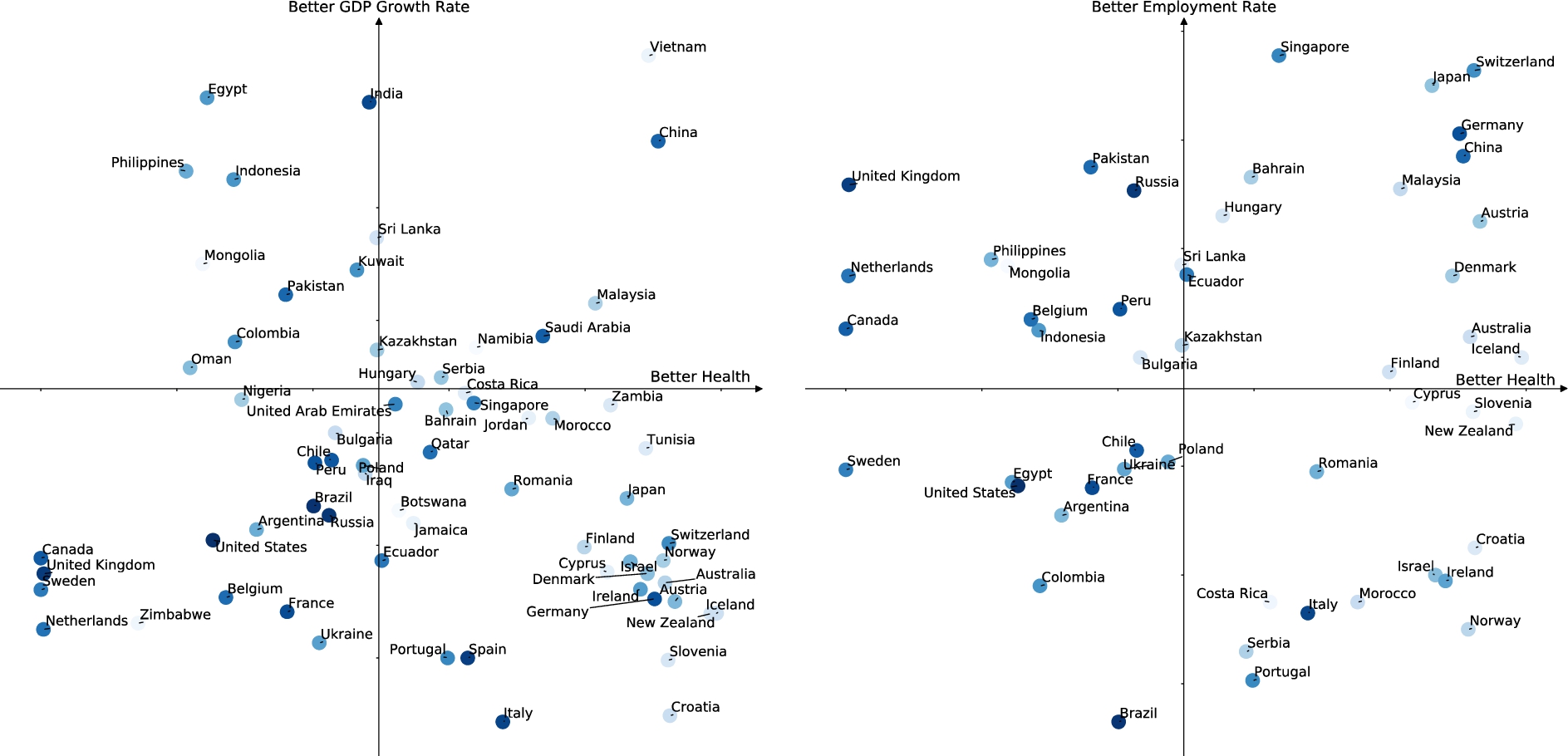
From Fig. 1 (left), Vietnam and China stood out with better situations in terms of both health and economic outcomes. These two countries were the very first to issue containment policies. The worst scenarios in both aspects were in the United States, the United Kingdom, Sweden, Netherlands, and a few other European countries. Most of these countries considered lock-down policy a bit too late when the infected number has been uncontrollably high.
Even though Italy, Spain, and Portugal were heavily suffered from the high number of confirmed COVID-19 cases during March and April, their lock-down policies had started to show some results as the ratio of recovered patients increases. The economies of these countries were still heavily suffered from this approach. Meanwhile, countries like Australia and New Zealand had effectively flattened the infection curve quite early on, and they also had to sacrifice their economic benefits, despite their early announcements of economic support policies in March.
Regarding the labour market in the right plot of Fig. 1, we can see a similar result for the United States, Sweden, France as their unemployment rates were significantly higher than in other countries. The labour market prospect was also dreadful in several nations with high numbers of COVID-19 cases, such as Brazil, Italy, and Portugal. Meanwhile, some other developed countries that already have a good general welfare pre-pandemic are showing the effectiveness of their support systems (e.g., Singapore, Switzerland, Japan, and Germany).
This initial data analysis shows that monetary and fiscal policies might play a vital role in economic recovery in the post-pandemic era. By June 2020, about 160 national governments had announced almost one thousand economic support policies. Had these monetary and fiscal measures substantially impacted these countries, causing early positive changes in economics and finance sectors during the COVID-19 pandemic, in terms of financial and labour market index? How strong were the causal effects? How the causal impact behave in different countries? Specifically, this analytical study aims to answer the following research questions:
Q1: What are the response and government policies amid the COVID-19 pandemic?
Q2: Did the government policies cause some impact on the financial market?
Q3: Did the economic support policies cause some impact on the financial market?
Q4: Did the economic support policies cause some impact on the labour market?
Since these economic and financial markets evolve in a time series manner amid the COVID-19 pandemic from 01/01/2020 to 22/03/2021, we aim to introduce a statistical machine learning method for such purpose, i.e., the causal inference over time series data and stochastic processes for 80 countries around the world. This causal analysis for the impact of economic support policies would significantly contribute to current literature, benefiting researchers, economists, policymakers, and international organizations interested in these topics.
2.Literature review
2.1.Research on impact of government policy
Regarding research on the impact of government policy during the COVID-19 pandemic, there have been some initial studies on the overall impact of all types of policies, focusing more on containment or health-related measures [7]. Their result showed that early containment policies such as school closure had significantly slowed down the infection rate, a similar conclusion to [31]. Other research also suggested that restriction on international travel is the biggest factor in preventing the virus spread [32] and reduces the health crisis impact.
Regarding the financial side of the crisis, several economists have analyzed how the COVID-19 pandemic affecting the world economy, using both real data and projected scenarios [10,15,16,18]. Baldwin and Tomiura [3] were focusing on the trade impact as several countries are still closing their borders. Some other researchers also initiate discussions on the impact on the stock market [22]. Other studies have been looking into some other financial indicators, particularly the foreign exchange markets [2] and gold and oil prices [17]. However, there has been not much research on the impact of monetary and fiscal policies for the COVID-19 pandemic on the economy, namely the financial and labour markets.
On the other hand, there have been numerous studies on the impact of monetary and fiscal policy for the last GFC [6,14,23]. Pastor and Veronesi [20] had analyzed the policies announced during the period 2007 to 2009 to measure their impacts on the stock market prices and volatility. They concluded that the policies had a negative effect on average, which means the market returns will go down on the announcement of the new policy. Ait-Sahalia et al. [1] also concluded that many of these measures had a negative impact, as the decisions to allow banks to fail, not to reduce the interest rate, or ad hoc bank bailouts tend to increase credit, liquidity risk and exacerbate market fears. It is worth noted that the GFC started from big banks and financial institutions, so the policies are quite different from the current COVID-19 crisis.
Moreover, both papers mentioned the uncertainty level as the key differentiation of the impact. The higher level of the surprise element, the worse the market returns would be. This is a big difference from the COVID-19 pandemic period as everyone is expecting benevolent responses from the governments, which minimizes the element of surprise. Pastor and Veronesi [20] also made a strong assumption in their model using a single-policy setting, while the real-world scenario of the COVID-19 pandemic had a multiple-policy setting. Furthermore, as these policies might not be effective immediately, it is worth considering a causal analysis of multiple different time lags and multiple-policy settings. This is the motivation for our causal inference approach for COVID-19 policy impact analysis in this paper.
2.2.Research on causal inference
The research about the causal relationship between two events has been extensively studied. In the past century, several different causality measures were proposed by statisticians and economists [9]. The earliest concept of causality for time series data was Granger causality, suggested by Granger [11]. Inspired by the Granger causality, different causality notions were suggested throughout the years, e.g., Sims causality [26], structural causality [33], and intervention causality [30].
Similar to Granger causality, Sims causality and structural causality also assume an observational framework. Meanwhile, intervention causality makes the much stronger assumption that intervention can be performed in the studies processes, which might be more suitable for a simulation environment rather than a real-life scenario like in our case. In this research, we use the Granger causality notion due to its proven effectiveness in multiple studies [24].
There are various approaches to causality inference, from classical statistical approaches to chaos and dynamic system theory approaches, with both parametric [19] and non-parametric causality measures [4,28]. In our specific context, we focus on the application of graphical approaches for causality inference in time series data as they are often used to model Granger causality in multivariate settings.
Some common graphical approaches for causality inference are SGS, PC, and FCI [27], which use principles of conditional dependence and application of the causal Markov condition to reconstruct the causal graph of the data generating process. SGS is considered as possibly more robust to nonlinearities, while the complexity of PC does not grow exponentially with the number of variables. The PC algorithm also cannot handle unobserved confounders, a problem which its extension, FCI, aims to remedy.
[25] considered these algorithms to be unsuitable to use with time series data, claiming the use of autocorrelation can lead to high false-positive rates. The authors suggested PCMCI, an advanced causality search algorithm, and claimed it is suitable for large datasets of variables featuring linear and nonlinear, time-delayed dependencies, given sample sizes of a few hundred or more, and that is showing consistency and higher detecting power with the reliable false positive control when compared with other algorithms. Therefore, we apply PCMCI with the Granger Causality notion to analyze the relationship and impact of government policy during the COVID-19 pandemic.
3.Methodology
3.1.Granger causality notion
Let X be a specific type of policy for a country (e.g. monetary support policy of a country) and Y be an index in the financial or labour markets (e.g. job index of a country). A naive interpretation of the problem may suggest simple approaches such as equating causality with high correlation. However, to infer the degree to which a variable X causes Y from the degree of X’s goodness as a predictor of Y, the problem turns out to be much more complex. As a result, rigorous ways to approach this question were developed in multiple causal inference research. Granger Causality, proposed by [11], is based on contrasting the ability to predict a stochastic process Y using all the information in the universe, denoted with U, with doing the same using all information in U except for some stochastic process X, denoted as
3.2.Graph-based causality inference
A graphical approach is often used to model Granger causality for multivariate time series where each time series is considered to be a node in a Granger network, with directed edges denoting a causal link, possibly with a delay in time. The main structure of an example graph-based causality search algorithm, PC algorithm, which was named after the authors, Peter Spirtes and Clark Glymour [27], consists of:
– Initialization: The full undirected graph over all variables
– Skeleton Construction: Afterwards, edges are eliminated by testing for conditional independence with increasing degrees of dependence. We only keep the connected variables.
– Edge elimination: Finally, a set of statistical and logical rules are applied to determine the direction of edges (i.e. the causality) in the graph.
3.3.PCMCI
PCMCI [25] is a graph-based causality search algorithm for multivariate time series, which contains two steps PC1 and MCI.
PC1:This is a Markov set discovery algorithm based on the above PC-stable algorithm [5] that eliminates irrelevant conditions in each time series through an iterative process of independence testing. Starting with preliminary parents
MCI: The Momentary Conditional Independence (MCI) test, which can address the false positive control for the highly-interdependent time series case, conditions on the parents of both variables in the potential causal link. To test whether lagged (back-shifted)
To explain the PCMCI method graphically, we illustrated the two steps in Fig. 2.
![Illustration of PCMCI algorithm (source: [25]).](https://ip.ios.semcs.net:443/media/web/2022/20-1/web-20-1-web210477/web-20-web210477-g002.jpg)
The left two diagrams illustrated the PC1 algorithms, with the blue and red colour edges represent the negative and positive causal links. The darker blue/red colour on each point of the time series indicates higher autocorrelation. Starting from a fully connected graph, all the weakest causal links between each time series pair are removed after each iteration step of the PC1 algorithms, which are the lightest shade of red and blue edges. We continue the iteration until there is no more condition to test. In this way, PC1 adaptively converges to typically only a few causal links left, denoted by darker blue and red edges. However, there might be some false positives (marked with a star). The MCI conditional independence test will further eliminate these false-positive links and generate the final graph with only significant causal links.
For example,
4.Data
For this research, we use a total of 13 types of times series from 01/01/2020 to 22/03/2021 to test our hypotheses. The time series for each country are extracted from the four datasets as below, whereas the statistics can be found in Table 1.
Table 1
Basic statistics of multiple time series in our data
| Symbol | Time series | mean | std | min | max |
| Active COVID-19 Cases | 2,429,524.1 | 6,299,581.9 | 0.0 | 29,276,571.0 | |
| Stringency Index | 55.0 | 25.3 | 0.0 | 100.0 | |
| Government Response Index | 51.4 | 22.4 | 0.0 | 89.8 | |
| Containment Health Index | 52.2 | 22.3 | 0.0 | 92.0 | |
| Economic Support Index | 46.7 | 31.9 | 0.0 | 100.0 | |
| Income Support policy | 1.0 | 0.8 | 0.0 | 2.0 | |
| Debt/Contract Relief policy | 1.1 | 0.8 | 0.0 | 2.0 | |
| Fiscal Measures policy (USD) | 247,639,703.3 | 13,627,454,739.5 | 0.0 | 1,957,600, 000, 000.0 | |
| International Support policy (USD) | 17,286,109.3 | 3,656,218,426.5 | 0.0 | 834,353,051, 822.0 | |
| New Jobless Claim (US labour market) | 188,616.1 | 200,882.1 | 28,714.3 | 981,000.0 | |
| Unemployment Rate (US labour market) | 6.5 | 4.7 | 1.2 | 17.1 | |
| Job Index (AU labour market) | 97.4 | 2.6 | 91.5 | 101.4 | |
| Wage Index (AU labour market) | 97.2 | 2.7 | 90.7 | 102.5 |
4.1.Oxford COVID-19 government response tracker (OxCGRT) dataset
The Oxford COVID-19 Government Response Tracker (OxCGRT) dataset [12] collected systematic information on which governments had taken which measures, and when. The data was collected for 179 countries and territories from 01/01/2020 to 22/03/2021, including these metrics: (1) COVID-19 Response Indexes: Stringency Index, Government Response Index, Containment Health Index, and Economic Support Index (see [12] for more information on the calculation of these indexes); (2) Economic Policies: Income Support, Debt/Contract Relief, Fiscal Measures, and International Support; (3) Containment and Closure policies: Close School, Close Workplace, Cancel public events, Restriction on gatherings, Close public transport, Stay at home requirements, Restrictions on internal movement, International travel control; and (4) Health System Policies: Public information campaigns, Testing policy, Contact tracing, Emergency Investment in healthcare, and Investment in vaccines. Within the scope of this paper, we focus on the “COVID-19 Response Indexes” and “Economic Policies”.
4.2.COVID-19 dataset
The COVID-19 Data was published by the Center for Systems Science and Engineering (CSSE) at Johns Hopkins University [8]. The dataset includes daily numbers of confirmed COVID-19 cases, deaths, recovered, active, new cases, new deaths, and new recovered for 186 countries and territories from 22/01/2020 to 22/03/2021. We used the number of Active cases from this dataset because we believe this number was the best figure to represent the current pandemic situation in each country. There were only a few countries with Active cases in the period between 01/01/2020 and 21/01/2020, and the difference between the number of total cases and active cases was not large (since the numbers of deaths/recovered are still low). Therefore, we used the number of confirmed cases from the OxCGRT dataset to fill the missing values for that period.
4.3.Financial market dataset
We first manually selected a major index to represent the financial market for each country in the OxCGRT dataset. However, not all countries and territories have such index and historical price data available. This was mainly due to the fact that some regions listed in the dataset did not have a stock exchange market (e.g. Vatican). Therefore, we had a final dataset with historical financial index close prices and trading volume from 01/01/2020 to 22/03/2021 for 80 countries. We then used Python to scrape these data from Investing.com. Table 5 in the appendix listed all the countries and their nominal financial indexes in the final dataset.
4.4.Labour market dataset
Since the labour market measures were different for each country, we had manually obtained the data for Australia and the United States for our analysis. The criteria to select these two countries are (1) the availability of high quality data and (2) countries with different labour markets and COVID-19 health situations (see Fig. 1). For consistency, these measures were also obtained for the period between 01/01/2020 and 22/03/2021.
For the United States, we obtained the weekly Unemployment Rates (Insured) and Initial Jobless Claims (Seasonally Adjusted) from the Federal Reserve Bank of St. Louis Economic Data (FRED).11 To transform weekly data into daily time series, we used the same Unemployment Rates and divide the weekly New Jobless Claims by 7 for each day in the previous week. The higher these measures were, the worse the United States labour market was at that point in time.
For Australia, we obtained the weekly Jobs Index and Wages Index from the Australian Bureau of Statistics (ABS).22 These estimates included indexes to present the changes in the labour market during the COVID-19 coronavirus period. To compare changes over time, the recorded 100th confirmed coronavirus case (i.e., the week ending 14th March 2020) was used as the reference time point for constructing the indexes and was given an index value of 100.0. To convert the data from weekly to daily time series, we use linear interpolation for any missing daily values. Opposite to the United States market, the higher these measures were, the better the Australian labour market was at that point in time.
5.Empirical analysis
We conducted multiple analyses to answer the four research questions.
5.1.The response and government policies amid the COVID-19 pandemic (Q1)
Nations worldwide had responded and announced multiple measures amid the COVID-19 pandemic. We focused on the economic support policies in this research and began with some descriptive statistics of our data. The countries in our final dataset had different numbers of Active COVID-19 cases and varying levels of government and economic support policies. Up until 22/03/2021, these 80 countries had announced 4741 different policies. Out of those, there were 1409 “Income Support” policies, 1616 “Debt/Contract Relief” policies, 1240 “Fiscal Measures” polices, and 476 “International Support” policies. Some of these policies were either replacing or updating the previous announcements, which were counted multiple times.
Most of these policies were similar among multiple nations, mainly focusing on the immediate financial assistance to workers and businesses suffered from the COVID-19 pandemic. Very few measures were taken for “International Support” at this point as most countries were prioritizing all resources to help the local businesses. We mentioned a few specific policies for some special cases in the footnote for the next part of our work (information sources for our analysis are from the datasets). From our statistic summary in Table 1, the average amount of monetary support for the domestic market was about 250 million USD, more than 14 times higher than that for international aid. This huge difference was explainable considering all countries were sharing the same situation with the recession, which forced them to focus more on national policies than international ones.
Let
5.2.Causal impact of government policies on the financial market (Q2)
We constructed a PCMCI causal inference model with seven time series:
From Table 2, we can see that the causal impact of different types of policies varied among countries. According to the number of total significant links by each index, more than 50% of these 80 countries could see some positive economic effects from the government responses. This was aligned with the analysis conclusion of the financial crisis 2007–2009 [20], which claimed that most policies have negative effects. The impact of COVID-19 responses might be delayed as the pandemic is still spreading in many countries. Even though the causal relationships were detected at varied time lags, the average was about 6 or 7 days for all significant links, which showed that the financial markets were quick in reacting to the COVID-19 policies.
There were 49 markets where significant causal links were detected with the general index
When we took a further look, some countries had a better economic recovery thanks to effective Containment and Health policies, denoted by significant causal links in column
On the contrary, many countries’ financial markets were impacted by
We also tested the causal effect of COVID-19 Response Indexes on market volatility. The average causal time lags of the impact on trading volumes were lower than the impact on the market prices, which indicated that the markets were sensitive at the current period of time, reacting quickly to new policy announcements. From our observation,
Table 2
Causal links of COVID-19 response indexes on financial market
| Financial Index Close Price | Trading Volume | |||||||||||||||
| Country | t-value | τ | t-value | τ | t-value | τ | t-value | τ | t-value | τ | t-value | τ | t-value | τ | t-value | τ |
| Argentina | 0.0921 | 6 | 0.0429 | 6 | 0.1064∗ | 6 | 0.1048∗ | 5 | 0.0952 | 13 | 0.0809 | 6 | 0.0735 | 13 | 0.0941 | 6 |
| Australia | 0.1989∗∗ | 1 | 0.1803∗∗ | 1 | 0.1727∗∗ | 1 | 0.2197∗∗ | 5 | 0.0203 | 11 | 0.0227 | 11 | 0.0230 | 11 | 0.0735 | 6 |
| Austria | 0.2107∗∗ | 8 | 0.1316∗∗ | 1 | 0.2005∗∗ | 8 | 0.2058∗∗ | 4 | 0.1787∗∗ | 4 | 0.0623 | 4 | 0.1619∗∗ | 4 | 0.1033∗ | 1 |
| Bahrain | 0.1158∗ | 7 | 0.0613 | 7 | 0.0638 | 7 | 0.0531 | 0 | 0.0722 | 1 | 0.0967∗ | 1 | 0.0658 | 1 | 0.2207∗∗ | 1 |
| Bangladesh | 0.1307∗∗ | 0 | 0.1215∗ | 0 | 0.1064∗ | 0 | 0.1677∗∗ | 0 | 0.0399 | 9 | 0.0437 | 9 | 0.0416 | 9 | 0.0500 | 14 |
| Belgium | 0.1209∗ | 10 | 0.0792 | 10 | 0.1180∗ | 10 | 0.1046∗ | 7 | 0.1008∗ | 2 | 0.0974∗ | 3 | 0.0852 | 3 | 0.1222∗ | 3 |
| B&H | 0.0047 | 7 | 0.0263 | 4 | 0.0000 | 0 | 0.0593 | 10 | 0.0499 | 9 | 0.0767 | 10 | 0.0821 | 10 | 0.1012∗ | 12 |
| Botswana | 0.0414 | 2 | 0.0460 | 2 | 0.0462 | 2 | 0.0166 | 4 | 0.0539 | 13 | 0.0405 | 13 | 0.0439 | 13 | 0.0668 | 2 |
| Brazil | 0.0444∗∗ | 4 | 0.0567∗∗ | 8 | 0.0213∗ | 4 | 0.0776∗∗ | 8 | 0.0342∗∗ | 9 | 0.0336∗∗ | 6 | 0.0420∗∗ | 10 | 0.0245∗∗ | 0 |
| Bulgaria | 0.1052∗ | 12 | 0.0917 | 3 | 0.0891 | 2 | 0.0615 | 4 | 0.1011∗ | 8 | 0.0311 | 6 | 0.1051∗ | 7 | 0.1157∗ | 1 |
| Canada | 0.1672∗∗ | 8 | 0.1483∗∗ | 8 | 0.1591∗∗ | 8 | 0.1016∗∗ | 9 | 0.0448∗∗ | 6 | 0.0579∗∗ | 6 | 0.0532∗∗ | 6 | 0.0549∗∗ | 6 |
| Chile | 0.0521 | 9 | 0.0370 | 9 | 0.0454 | 10 | 0.0156 | 12 | 0.1013∗ | 4 | 0.1101∗ | 4 | 0.1069∗ | 4 | 0.1245∗ | 4 |
| China | 0.0769 | 3 | 0.0841 | 3 | 0.0794 | 0 | 0.0568 | 11 | 0.1101∗ | 9 | 0.1071∗ | 9 | 0.1088∗ | 9 | 0.0711 | 10 |
| Colombia | 0.1916∗∗ | 1 | 0.1441∗∗ | 9 | 0.1393∗∗ | 1 | 0.2757∗∗ | 8 | 0.0292 | 13 | 0.0457 | 12 | 0.0536 | 12 | 0.0698 | 2 |
| Costa Rica | 0.0138 | 3 | 0.0175 | 3 | 0.0111 | 3 | 0.0176 | 0 | 0.0139 | 3 | 0.0176 | 3 | 0.0111 | 3 | 0.0176 | 0 |
| Croatia | 0.1220∗ | 4 | 0.1135∗ | 14 | 0.1208∗ | 14 | 0.1315∗∗ | 5 | 0.0930 | 14 | 0.1264∗ | 14 | 0.0853 | 14 | 0.1467∗∗ | 14 |
| Cyprus | 0.0270 | 14 | 0.0639 | 2 | 0.0385 | 1 | 0.0740 | 9 | 0.1233∗ | 4 | 0.0883 | 4 | 0.0913 | 11 | 0.1553∗∗ | 6 |
| Denmark | 0.0936 | 4 | 0.0915 | 4 | 0.0923 | 4 | 0.0911 | 12 | 0.1832∗∗ | 9 | 0.1693∗∗ | 9 | 0.1767∗∗ | 9 | 0.0935 | 3 |
| Ecuador | 0.0428 | 0 | 0.0573 | 8 | 0.0579 | 8 | 0.0391 | 8 | 0.0969∗ | 12 | 0.1047∗ | 12 | 0.1012∗ | 12 | 0.1116∗ | 10 |
| Egypt | 0.1027∗ | 6 | 0.0856 | 3 | 0.0985∗ | 13 | 0.1686∗∗ | 0 | 0.0320 | 13 | 0.0577 | 13 | 0.0561 | 13 | 0.0428 | 9 |
| Finland | 0.1414∗∗ | 13 | 0.0808 | 13 | 0.0964∗ | 13 | 0.0994∗ | 8 | 0.3134∗∗ | 9 | 0.3434∗∗ | 9 | 0.3480∗∗ | 9 | 0.2840∗∗ | 9 |
| France | 0.1617∗∗ | 3 | 0.1182∗ | 8 | 0.1470∗∗ | 3 | 0.1411∗∗ | 8 | 0.1366∗∗ | 10 | 0.0717 | 10 | 0.1276∗∗ | 10 | 0.0885 | 4 |
| Germany | 0.0943 | 8 | 0.1182∗ | 8 | 0.1073∗ | 8 | 0.1022∗ | 8 | 0.1653∗∗ | 2 | 0.1181∗ | 0 | 0.1153∗ | 0 | 0.1053∗ | 4 |
| Greece | 0.0832 | 10 | 0.1087∗ | 14 | 0.1112∗ | 14 | 0.1415∗∗ | 12 | 0.0855 | 2 | 0.0456 | 3 | 0.0454 | 3 | 0.0386 | 6 |
| Hungary | 0.1150∗ | 4 | 0.0988∗ | 4 | 0.1224∗ | 4 | 0.1483∗∗ | 6 | 0.0049 | 9 | 0.0140 | 2 | 0.0223 | 9 | 0.0640 | 6 |
| Iceland | 0.1428∗∗ | 9 | 0.1658∗∗ | 4 | 0.1322∗∗ | 4 | 0.1346∗∗ | 3 | 0.0462 | 11 | 0.1936∗∗ | 1 | 0.2561∗∗ | 1 | 0.4003∗∗ | 0 |
| India | 0.2795∗∗ | 0 | 0.2876∗∗ | 0 | 0.2826∗∗ | 0 | 0.0800 | 12 | 0.0866 | 2 | 0.0996∗ | 0 | 0.0968∗ | 0 | 0.1680∗∗ | 4 |
| Indonesia | 0.0768 | 12 | 0.0776 | 12 | 0.0810 | 12 | 0.0757 | 5 | 0.0935 | 0 | 0.1094∗ | 0 | 0.1087∗ | 0 | 0.0957 | 0 |
| Iraq | 0.0370 | 9 | 0.0618 | 9 | 0.0580 | 9 | 0.0114 | 8 | 0.0718 | 7 | 0.0716 | 5 | 0.0826 | 5 | 0.0707 | 10 |
| Ireland | 0.1388∗∗ | 13 | 0.1384∗∗ | 13 | 0.1043∗ | 13 | 0.1057∗ | 13 | 0.0443 | 8 | 0.0341 | 10 | 0.0318 | 8 | 0.0556 | 7 |
| Israel | 0.1202∗ | 11 | 0.1354∗∗ | 11 | 0.1272∗∗ | 11 | 0.1952∗∗ | 7 | 0.0457 | 5 | 0.0474 | 6 | 0.0463 | 6 | 0.0825 | 8 |
| Italy | 0.1194∗ | 10 | 0.1155∗ | 10 | 0.1183∗ | 10 | 0.1317∗∗ | 7 | 0.1344∗∗ | 5 | 0.1325∗∗ | 5 | 0.1317∗∗ | 5 | 0.1035∗ | 3 |
| Jamaica | 0.1219∗ | 9 | 0.1406∗∗ | 9 | 0.1450∗∗ | 9 | 0.0766 | 13 | 0.2185∗∗ | 13 | 0.2344∗∗ | 13 | 0.2243∗∗ | 13 | 0.0696 | 13 |
| Japan | 0.0438 | 8 | 0.1100∗ | 9 | 0.0486 | 9 | 0.1361∗∗ | 9 | 0.1164∗ | 7 | 0.1232∗ | 7 | 0.1266∗∗ | 7 | 0.1090∗ | 6 |
| Jordan | 0.1028∗ | 2 | 0.1288∗∗ | 2 | 0.1199∗ | 2 | 0.1129∗ | 14 | 0.0073 | 8 | 0.0068 | 2 | 0.0084 | 2 | 0.0102 | 6 |
| Kazakhstan | 0.1277∗∗ | 2 | 0.1123∗ | 3 | 0.1232∗ | 3 | 0.1002∗ | 2 | 0.0610 | 4 | 0.0645 | 14 | 0.0741 | 9 | 0.0987∗ | 11 |
| Kenya | 0.1010∗ | 14 | 0.1196∗ | 14 | 0.1354∗∗ | 14 | 0.0744 | 9 | 0.0841 | 2 | 0.1101∗ | 2 | 0.1207∗ | 2 | 0.0756 | 12 |
| Kuwait | 0.1491∗∗ | 8 | 0.2238∗∗ | 10 | 0.2251∗∗ | 10 | 0.0726 | 11 | 0.0840 | 6 | 0.0858 | 6 | 0.0839 | 6 | 0.0454 | 14 |
| Lebanon | 0.1659∗∗ | 13 | 0.1809∗∗ | 13 | 0.1783∗∗ | 13 | 0.1478∗∗ | 13 | 0.1048∗ | 13 | 0.0900 | 13 | 0.0914 | 13 | 0.0265 | 8 |
| Malaysia | 0.1809∗∗ | 2 | 0.1390∗∗ | 6 | 0.1247∗ | 2 | 0.0841 | 6 | 0.1081∗ | 7 | 0.1084∗ | 7 | 0.1259∗ | 7 | 0.0389 | 14 |
| Mauritius | 0.0920 | 13 | 0.0781 | 13 | 0.0794 | 13 | 0.1578∗∗ | 7 | 0.0328 | 9 | 0.0510 | 9 | 0.0500 | 9 | 0.0736 | 2 |
| Mongolia | 0.0449 | 3 | 0.0501 | 3 | 0.0465 | 3 | 0.0473 | 13 | 0.1724∗∗ | 0 | 0.1664∗∗ | 0 | 0.1576∗∗ | 0 | 0.0863 | 10 |
| Morocco | 0.1140∗ | 10 | 0.0528 | 9 | 0.0522 | 6 | 0.0613 | 5 | 0.0749 | 1 | 0.0723 | 1 | 0.0873 | 1 | 0.0732 | 1 |
| Namibia | 0.1119∗ | 6 | 0.0721 | 6 | 0.0804 | 6 | 0.0000 | 0 | 0.1276∗∗ | 8 | 0.0795 | 8 | 0.0737 | 8 | 0.0551 | 14 |
| Netherlands | 0.1147∗ | 10 | 0.0747 | 9 | 0.0862 | 10 | 0.1748∗∗ | 7 | 0.1353∗∗ | 0 | 0.1687∗∗ | 0 | 0.1298∗∗ | 0 | 0.1670∗∗ | 3 |
| New Zealand | 0.1307∗∗ | 1 | 0.1387∗∗ | 1 | 0.1356∗∗ | 1 | 0.2224∗∗ | 7 | 0.0616 | 5 | 0.0687 | 0 | 0.0554 | 5 | 0.0958 | 3 |
Table 2
(Continued)
| Financial Index Close Price | Trading Volume | |||||||||||||||
| Country | t-value | τ | t-value | τ | t-value | τ | t-value | τ | t-value | τ | t-value | τ | t-value | τ | t-value | τ |
| Niger | 0.0464 | 7 | 0.0778 | 7 | 0.0926 | 7 | 0.0601 | 9 | 0.0568 | 9 | 0.0471 | 9 | 0.0383 | 9 | 0.0611 | 6 |
| Nigeria | 0.0886 | 2 | 0.0845 | 2 | 0.0715 | 9 | 0.0575 | 2 | 0.0896 | 2 | 0.0800 | 2 | 0.0648 | 2 | 0.1339∗∗ | 14 |
| Norway | 0.1119∗ | 7 | 0.0938 | 14 | 0.0975∗ | 14 | 0.1211∗ | 4 | 0.0669 | 1 | 0.0867 | 1 | 0.1012∗ | 1 | 0.0634 | 0 |
| Oman | 0.0403 | 3 | 0.0751 | 3 | 0.0673 | 3 | 0.0363 | 6 | 0.2649∗∗ | 4 | 0.2464∗∗ | 4 | 0.2717∗∗ | 4 | 0.0000 | 0 |
| Pakistan | 0.1561∗∗ | 8 | 0.1442∗∗ | 8 | 0.1410∗∗ | 8 | 0.1494∗∗ | 1 | 0.0737 | 7 | 0.0781 | 12 | 0.0711 | 13 | 0.1034∗ | 12 |
| Peru | 0.0985∗ | 10 | 0.1111∗ | 10 | 0.0965∗ | 10 | 0.1087∗ | 13 | 0.1072∗ | 1 | 0.0639 | 9 | 0.0689 | 9 | 0.1127∗ | 13 |
| Philippines | 0.1385∗∗ | 5 | 0.0950 | 11 | 0.1042∗ | 5 | 0.1085∗ | 0 | 0.0700 | 10 | 0.0686 | 3 | 0.0670 | 3 | 0.0502 | 5 |
| Poland | 0.0965∗ | 10 | 0.0857 | 10 | 0.0692 | 10 | 0.0854 | 10 | 0.1174∗ | 3 | 0.1360∗∗ | 9 | 0.1266∗∗ | 9 | 0.1374∗∗ | 9 |
| Portugal | 0.1271∗∗ | 5 | 0.0866 | 10 | 0.0965 | 10 | 0.2205∗∗ | 4 | 0.0897 | 14 | 0.1085∗ | 0 | 0.1041∗ | 14 | 0.1280∗∗ | 11 |
| Qatar | 0.0829 | 10 | 0.1047∗ | 10 | 0.0831 | 10 | 0.1142∗ | 10 | 0.1339∗∗ | 6 | 0.1424∗∗ | 6 | 0.1385∗∗ | 6 | 0.1056∗ | 6 |
| Romania | 0.1027∗ | 12 | 0.1321∗∗ | 12 | 0.1362∗∗ | 12 | 0.1213∗ | 8 | 0.0828 | 13 | 0.0832 | 13 | 0.0737 | 13 | 0.0523 | 12 |
| Russia | 0.1822∗∗ | 3 | 0.0593 | 14 | 0.0338 | 14 | 0.0868 | 1 | 0.1259∗∗ | 10 | 0.0727 | 10 | 0.0698 | 4 | 0.0569 | 6 |
| Rwanda | 0.0577 | 4 | 0.0494 | 4 | 0.0490 | 4 | 0.0007 | 0 | 0.0455 | 9 | 0.0448 | 9 | 0.0488 | 9 | 0.0557 | 8 |
| Saudi Arabia | 0.0922 | 11 | 0.0779 | 8 | 0.0882 | 9 | 0.0547 | 11 | 0.0492 | 4 | 0.0589 | 4 | 0.0467 | 4 | 0.0233 | 7 |
| Serbia | 0.1544∗∗ | 9 | 0.1538∗∗ | 9 | 0.1589∗∗ | 9 | 0.1608∗∗ | 1 | 0.0613 | 2 | 0.0620 | 5 | 0.0732 | 1 | 0.0575 | 5 |
| Singapore | 0.0766 | 6 | 0.0592 | 6 | 0.0763 | 4 | 0.0650 | 13 | 0.0628 | 7 | 0.0639 | 11 | 0.0590 | 11 | 0.2357∗∗ | 10 |
| Slovenia | 0.0577 | 9 | 0.0692 | 9 | 0.0707 | 9 | 0.0721 | 7 | 0.0508 | 7 | 0.0450 | 7 | 0.0414 | 7 | 0.0565 | 7 |
| South Africa | 0.1144∗ | 10 | 0.1087∗ | 10 | 0.1088∗ | 10 | 0.1038∗ | 7 | 0.1434∗∗ | 4 | 0.1394∗∗ | 4 | 0.1256∗ | 4 | 0.3924∗∗ | 0 |
| Spain | 0.1212∗ | 10 | 0.1325∗∗ | 5 | 0.1461∗∗ | 5 | 0.1834∗∗ | 7 | 0.0894 | 6 | 0.0809 | 2 | 0.0838 | 6 | 0.0638 | 3 |
| Sri Lanka | 0.0489 | 10 | 0.0542 | 10 | 0.0560 | 10 | 0.0430 | 11 | 0.0324 | 0 | 0.0464 | 8 | 0.0544 | 8 | 0.0145 | 2 |
| Sweden | 0.1975∗∗ | 12 | 0.1723∗∗ | 12 | 0.2115∗∗ | 12 | 0.1316∗∗ | 13 | 0.2843∗∗ | 0 | 0.2283∗∗ | 0 | 0.2457∗∗ | 0 | 0.2505∗∗ | 1 |
| Switzerland | 0.0734 | 2 | 0.0625 | 9 | 0.0684 | 9 | 0.1273∗∗ | 5 | 0.1703∗∗ | 3 | 0.1304∗∗ | 3 | 0.1666∗∗ | 3 | 0.2095∗∗ | 1 |
| Thailand | 0.1545∗∗ | 14 | 0.0662 | 14 | 0.1088∗ | 14 | 0.1298∗∗ | 6 | 0.0657 | 14 | 0.0540 | 0 | 0.0645 | 14 | 0.1093∗ | 0 |
| Tunisia | 0.1101∗ | 6 | 0.0972∗ | 6 | 0.1015∗ | 6 | 0.0754 | 2 | 0.0258 | 6 | 0.0199 | 0 | 0.0229 | 4 | 0.0528 | 5 |
| Turkey | 0.0920 | 8 | 0.0706 | 8 | 0.0742 | 8 | 0.0530 | 2 | 0.0955 | 8 | 0.0692 | 5 | 0.0938 | 8 | 0.0982∗ | 2 |
| Uganda | 0.0993∗ | 1 | 0.1139∗ | 1 | 0.1265∗∗ | 1 | 0.1441∗∗ | 4 | 0.0628 | 11 | 0.0783 | 11 | 0.0659 | 11 | 0.0937 | 2 |
| Ukraine | 0.0204 | 11 | 0.0016 | 10 | 0.0023 | 5 | 0.0000 | 0 | 0.0678 | 9 | 0.1022∗ | 9 | 0.0995∗ | 9 | 0.1009∗ | 0 |
| UAE | 0.1519∗∗ | 2 | 0.0625 | 9 | 0.1032∗ | 9 | 0.1371∗∗ | 6 | 0.0507 | 2 | 0.0690 | 2 | 0.0642 | 2 | 0.0746 | 2 |
| UK | 0.0543∗ | 2 | 0.0445∗ | 2 | 0.0324 | 2 | 0.1045∗∗ | 5 | 0.1624∗∗ | 11 | 0.1752∗∗ | 11 | 0.0809∗∗ | 11 | 0.1104∗∗ | 11 |
| US | 0.0431∗∗ | 8 | 0.0366∗∗ | 4 | 0.0575∗∗ | 2 | 0.0607∗∗ | 10 | 0.0082 | 6 | 0.0115 | 6 | 0.0121 | 6 | 0.0106 | 9 |
| Venezuela | 0.0803 | 4 | 0.0806 | 4 | 0.0813 | 4 | 0.0375 | 10 | 0.1452∗∗ | 8 | 0.1365∗∗ | 8 | 0.1467∗∗ | 8 | 0.1095∗ | 4 |
| Vietnam | 0.0887 | 7 | 0.0825 | 0 | 0.0885 | 7 | 0.0874 | 13 | 0.0598 | 1 | 0.0697 | 1 | 0.0696 | 1 | 0.1540∗∗ | 9 |
| Zambia | 0.1616∗∗ | 0 | 0.1389∗∗ | 0 | 0.1428∗∗ | 0 | 0.0855 | 12 | 0.1372∗∗ | 13 | 0.1214∗ | 13 | 0.1314∗∗ | 13 | 0.0990∗ | 8 |
| Zimbabwe | 0.0416 | 4 | 0.0623 | 4 | 0.0591 | 4 | 0.0052 | 0 | 0.1157∗ | 11 | 0.1205∗ | 2 | 0.1104∗ | 2 | 0.1806∗∗ | 2 |
| Total links | 49 | 38 | 43 | 43 | 33 | 33 | 34 | 37 | ||||||||
| Mean lags τ | 6.8 | 7.2 | 7.0 | 6.8 | 6.8 | 6.1 | 6.8 | 6.0 | ||||||||
Note: * and ** denote significant links at 95% and 99% confidence levels respectively.
Table 3
Causal links of economic policies on financial market
| Financial Index Close Price | Trading Volume | |||||||||||||||
| Country | t-value | τ | t-value | τ | t-value | τ | t-value | τ | t-value | τ | t-value | τ | t-value | τ | t-value | τ |
| Argentina | 0.0593 | 2 | 0.0368 | 3 | 0.1170∗ | 8 | 0.0711 | 0 | 0.1112∗ | 9 | 0.0845 | 7 | 0.0710 | 8 | 0.0618 | 12 |
| Australia | 0.1733∗∗ | 5 | 0.1641∗∗ | 0 | 0.1955∗∗ | 8 | 0.0704 | 2 | 0.1516∗∗ | 2 | 0.0958 | 2 | 0.0999∗ | 9 | 0.1357∗∗ | 0 |
| Austria | 0.0945 | 10 | 0.1857∗∗ | 3 | 0.1990∗∗ | 2 | 0.0572 | 6 | 0.0351 | 14 | 0.0993∗ | 4 | 0.1831∗∗ | 2 | 0.1412∗∗ | 2 |
| Bahrain | 0.1402∗∗ | 13 | 0.0557 | 0 | 0.1761∗∗ | 2 | 0.0513 | 0 | 0.5393∗∗ | 1 | 0.2040∗∗ | 14 | 0.0449 | 7 | 0.0381 | 6 |
| Bangladesh | 0.0002 | 12 | 0.1404∗∗ | 0 | 0.0147 | 0 | 0.0153 | 3 | 0.0627 | 0 | 0.0729 | 7 | 0.0632 | 5 | 0.1154∗ | 13 |
| Belgium | 0.1817∗∗ | 7 | 0.0768 | 13 | 0.1389∗∗ | 4 | 0.0693 | 14 | 0.1242∗ | 14 | 0.0565 | 6 | 0.2176∗∗ | 0 | 0.1447∗∗ | 4 |
| B&H | 0.0731 | 10 | 0.0731 | 10 | 0.1548∗∗ | 13 | 0.1148∗ | 12 | 0.1425∗∗ | 3 | 0.1425∗∗ | 3 | 0.1081∗ | 6 | 0.0412 | 2 |
| Botswana | 0.0709 | 11 | 0.0091 | 4 | 0.0288 | 9 | 0.1166∗ | 7 | 0.0769 | 10 | 0.0361 | 5 | 0.1281∗∗ | 0 | 0.0771 | 5 |
| Brazil | 0.0157 | 12 | 0.0840∗∗ | 7 | 0.0190∗ | 6 | 0.0240∗∗ | 5 | 0.0106 | 6 | 0.0310∗∗ | 0 | 0.0047 | 2 | 0.0110 | 10 |
| Bulgaria | 0.0813 | 10 | 0.1042∗ | 14 | 0.1541∗∗ | 5 | 0.0743 | 13 | 0.1319∗∗ | 0 | 0.1339∗∗ | 7 | 0.1269∗∗ | 13 | 0.1119∗ | 11 |
| Canada | 0.1713∗∗ | 9 | 0.0490∗∗ | 5 | 0.0189 | 6 | 0.0108 | 3 | 0.0912∗∗ | 6 | 0.0318∗ | 6 | 0.0359∗∗ | 0 | 0.0294∗ | 4 |
| Chile | 0.0361 | 7 | 0.0600 | 4 | 0.1629∗∗ | 0 | 0.0301 | 2 | 0.0415 | 0 | 0.0596 | 0 | 0.1191∗ | 5 | 0.0501 | 11 |
| China | 0.1020∗ | 3 | 0.0728 | 3 | 0.0779 | 4 | 0.0842 | 14 | 0.0406 | 1 | 0.0736 | 0 | 0.0943 | 11 | 0.0653 | 14 |
| Colombia | 0.0674 | 1 | 0.3259∗∗ | 8 | 0.1194∗ | 6 | 0.0556 | 9 | 0.0930 | 5 | 0.1002∗ | 8 | 0.0640 | 3 | 0.0662 | 9 |
| Costa Rica | 0.0116 | 0 | 0.0255 | 0 | 0.0000 | 0 | 0.0417 | 0 | 0.0117 | 0 | 0.0256 | 0 | 0.0000 | 0 | 0.0417 | 0 |
| Croatia | 0.1420∗∗ | 5 | 0.1123∗ | 8 | 0.0757 | 1 | 0.1208∗ | 10 | 0.0550 | 9 | 0.0489 | 11 | 0.0667 | 2 | 0.0822 | 0 |
| Cyprus | 0.0657 | 2 | 0.0755 | 9 | 0.1010∗ | 2 | 0.1120∗ | 7 | 0.0419 | 10 | 0.0661 | 6 | 0.0927 | 1 | 0.0443 | 4 |
| Denmark | 0.0972∗ | 4 | 0.0844 | 12 | 0.1176∗ | 4 | 0.0637 | 3 | 0.1198∗ | 9 | 0.0314 | 10 | 0.0809 | 12 | 0.0546 | 13 |
| Ecuador | 0.0332 | 8 | 0.0222 | 8 | 0.0246 | 12 | 0.1140∗ | 5 | 0.1212∗ | 5 | 0.1420∗∗ | 5 | 0.0803 | 1 | 0.0876 | 3 |
| Egypt | 0.1592∗∗ | 7 | 0.2225∗∗ | 0 | 0.1042∗ | 0 | 0.0610 | 1 | 0.0508 | 9 | 0.0478 | 0 | 0.0637 | 7 | 0.1072∗ | 3 |
| Finland | 0.1440∗∗ | 8 | 0.0999∗ | 11 | 0.0966∗ | 11 | 0.1164∗ | 13 | 0.2479∗∗ | 9 | 0.2444∗∗ | 9 | 0.0733 | 13 | 0.0600 | 0 |
| France | 0.2282∗∗ | 8 | 0.1305∗∗ | 8 | 0.1254∗ | 6 | 0.0911 | 8 | 0.1866∗∗ | 0 | 0.0968∗ | 4 | 0.0523 | 2 | 0.0451 | 0 |
| Germany | 0.0853 | 3 | 0.0435 | 13 | 0.2443∗∗ | 1 | 0.1090∗ | 14 | 0.1149∗ | 4 | 0.0980∗ | 2 | 0.0484 | 2 | 0.0959 | 2 |
| Greece | 0.1138∗ | 1 | 0.1210∗ | 12 | 0.0962 | 1 | 0.0306 | 10 | 0.0226 | 7 | 0.0540 | 5 | 0.0583 | 6 | 0.0776 | 0 |
| Hungary | 0.0998∗ | 13 | 0.1550∗∗ | 6 | 0.0775 | 3 | 0.0758 | 13 | 0.0999∗ | 13 | 0.0980∗ | 4 | 0.1033∗ | 13 | 0.0865 | 13 |
| Iceland | 0.0585 | 9 | 0.1293∗∗ | 3 | 0.1150∗ | 5 | 0.0691 | 2 | 0.1106∗ | 11 | 0.4180∗∗ | 0 | 0.0000 | 0 | 0.1258∗ | 5 |
| India | 0.1203∗ | 0 | 0.1632∗∗ | 12 | 0.0511 | 1 | 0.0454 | 4 | 0.1328∗∗ | 6 | 0.2430∗∗ | 5 | 0.0809 | 6 | 0.0241 | 12 |
| Indonesia | 0.0835 | 7 | 0.1321∗∗ | 5 | 0.1304∗∗ | 5 | 0.0434 | 0 | 0.1057∗ | 7 | 0.0941 | 0 | 0.0846 | 11 | 0.0978∗ | 11 |
| Iraq | 0.0829 | 14 | 0.0829 | 14 | 0.0090 | 8 | 0.1370∗∗ | 1 | 0.0123 | 2 | 0.0123 | 2 | 0.0930 | 7 | 0.0789 | 0 |
| Ireland | 0.0995∗ | 13 | 0.0992∗ | 6 | 0.1024∗ | 6 | 0.1016∗ | 13 | 0.0584 | 7 | 0.0146 | 7 | 0.0127 | 11 | 0.0395 | 0 |
| Israel | 0.1347∗∗ | 6 | 0.0710 | 11 | 0.1329∗∗ | 7 | 0.1034∗ | 0 | 0.0403 | 7 | 0.0823 | 10 | 0.1012∗ | 3 | 0.1135∗ | 9 |
| Italy | 0.1571∗∗ | 7 | 0.1149∗ | 7 | 0.0779 | 0 | 0.0451 | 4 | 0.0815 | 3 | 0.1132∗ | 3 | 0.0660 | 1 | 0.0867 | 10 |
| Jamaica | 0.0867 | 12 | 0.0627 | 13 | 0.2097∗∗ | 14 | 0.0700 | 0 | 0.0688 | 12 | 0.0766 | 6 | 0.3459∗∗ | 9 | 0.0682 | 12 |
| Japan | 0.2110∗∗ | 1 | 0.1567∗∗ | 9 | 0.0628 | 1 | 0.1281∗∗ | 4 | 0.0936 | 14 | 0.1430∗∗ | 6 | 0.0381 | 10 | 0.0261 | 12 |
| Jordan | 0.0995∗ | 0 | 0.1181∗ | 14 | 0.0222 | 5 | 0.0942 | 12 | 0.0080 | 9 | 0.0101 | 6 | 0.0000 | 0 | 0.0859 | 8 |
| Kazakhstan | 0.1486∗∗ | 14 | 0.1385∗∗ | 3 | 0.1671∗∗ | 1 | 0.0670 | 14 | 0.0671 | 1 | 0.1496∗∗ | 2 | 0.0964∗ | 12 | 0.0853 | 5 |
| Kenya | 0.0693 | 6 | 0.1441∗∗ | 7 | 0.0408 | 7 | 0.1044∗ | 8 | 0.0493 | 3 | 0.1358∗∗ | 2 | 0.0460 | 8 | 0.0726 | 14 |
| Kuwait | 0.1371∗∗ | 13 | 0.0997∗ | 11 | 0.1183∗ | 8 | 0.0777 | 8 | 0.0495 | 8 | 0.0655 | 14 | 0.0611 | 3 | 0.0786 | 1 |
| Lebanon | 0.0876 | 9 | 0.1541∗∗ | 13 | 0.0865 | 0 | 0.0161 | 0 | 0.0579 | 0 | 0.0286 | 8 | 0.0554 | 0 | 0.0035 | 13 |
| Malaysia | 0.0702 | 10 | 0.0936 | 6 | 0.0901 | 4 | 0.1029∗ | 11 | 0.0952 | 6 | 0.0760 | 6 | 0.1067∗ | 4 | 0.0864 | 6 |
| Mauritius | 0.1226∗ | 9 | 0.1474∗∗ | 7 | 0.0531 | 0 | 0.0498 | 9 | 0.0827 | 10 | 0.1011∗ | 12 | 0.0766 | 8 | 0.0723 | 9 |
| Mongolia | 0.0961 | 13 | 0.0953 | 1 | 0.0281 | 14 | 0.0548 | 1 | 0.1042∗ | 14 | 0.1137∗ | 11 | 0.0624 | 4 | 0.0275 | 3 |
| Morocco | 0.1278∗∗ | 0 | 0.0821 | 5 | 0.0345 | 8 | 0.0632 | 14 | 0.0779 | 3 | 0.0634 | 14 | 0.1430∗∗ | 8 | 0.0614 | 4 |
| Namibia | 0.0004 | 12 | 0.0000 | 0 | 0.0004 | 12 | 0.0922 | 3 | 0.0742 | 7 | 0.1189∗ | 4 | 0.0742 | 7 | 0.0681 | 1 |
| Netherlands | 0.2372∗∗ | 7 | 0.0794 | 11 | 0.0937 | 14 | 0.0694 | 7 | 0.4137∗∗ | 3 | 0.1063∗ | 3 | 0.1500∗∗ | 3 | 0.0260 | 9 |
| New Zealand | 0.1201∗ | 13 | 0.0640 | 7 | 0.2644∗∗ | 7 | 0.0788 | 2 | 0.1064∗ | 4 | 0.0780 | 2 | 0.1763∗∗ | 3 | 0.0912 | 7 |
Table 3
(Continued)
| Financial Index Close Price | Trading Volume | |||||||||||||||
| Country | t-value | τ | t-value | τ | t-value | τ | t-value | τ | t-value | τ | t-value | τ | t-value | τ | t-value | τ |
| Niger | 0.1150∗ | 6 | 0.0684 | 9 | 0.1136∗ | 1 | 0.0991∗ | 9 | 0.0740 | 6 | 0.0394 | 9 | 0.0515 | 0 | 0.0503 | 5 |
| Nigeria | 0.0885 | 2 | 0.0327 | 12 | 0.0870 | 0 | 0.1312∗∗ | 7 | 0.1263∗ | 14 | 0.1180∗ | 0 | 0.1040∗ | 13 | 0.0634 | 0 |
| Norway | 0.0975∗ | 4 | 0.1491∗∗ | 1 | 0.1610∗∗ | 3 | 0.0748 | 14 | 0.0533 | 11 | 0.1158∗ | 6 | 0.0630 | 4 | 0.0291 | 12 |
| Oman | 0.0641 | 8 | 0.0736 | 10 | 0.0410 | 2 | 0.0381 | 12 | 0.4205∗∗ | 0 | 0.0079 | 5 | 0.2721∗∗ | 1 | 0.0704 | 5 |
| Pakistan | 0.1842∗∗ | 8 | 0.1573∗∗ | 1 | 0.1637∗∗ | 9 | 0.0419 | 4 | 0.0633 | 5 | 0.0680 | 8 | 0.0715 | 10 | 0.0590 | 13 |
| Peru | 0.1193∗ | 9 | 0.0805 | 13 | 0.1020∗ | 7 | 0.1172∗ | 4 | 0.1038∗ | 2 | 0.1212∗ | 8 | 0.1107∗ | 0 | 0.0542 | 2 |
| Philippines | 0.1025∗ | 4 | 0.0977∗ | 0 | 0.1312∗∗ | 9 | 0.0973∗ | 8 | 0.0553 | 2 | 0.0623 | 5 | 0.0477 | 7 | 0.0870 | 11 |
| Poland | 0.0732 | 10 | 0.1374∗∗ | 12 | 0.1257∗ | 6 | 0.1353∗∗ | 10 | 0.1313∗∗ | 9 | 0.1227∗ | 9 | 0.2181∗∗ | 2 | 0.0843 | 6 |
| Portugal | 0.2168∗∗ | 11 | 0.1747∗∗ | 4 | 0.0968∗ | 8 | 0.0693 | 2 | 0.1362∗∗ | 7 | 0.1215∗ | 11 | 0.0805 | 6 | 0.0222 | 1 |
| Qatar | 0.1778∗∗ | 10 | 0.0543 | 6 | 0.1443∗∗ | 9 | 0.0960 | 1 | 0.1111∗ | 6 | 0.1161∗ | 6 | 0.0863 | 3 | 0.1093∗ | 1 |
| Romania | 0.0786 | 10 | 0.1224∗ | 8 | 0.1951∗∗ | 5 | 0.1021∗ | 12 | 0.0747 | 12 | 0.0375 | 3 | 0.0572 | 14 | 0.0673 | 13 |
| Russia | 0.0670 | 14 | 0.0625 | 8 | 0.0960 | 8 | 0.0564 | 0 | 0.0794 | 7 | 0.0887 | 6 | 0.1057∗ | 10 | 0.0789 | 13 |
| Rwanda | 0.0017 | 7 | 0.0000 | 8 | 0.0175 | 12 | 0.0560 | 0 | 0.0765 | 6 | 0.0810 | 4 | 0.1155∗ | 10 | 0.0937 | 0 |
| Saudi Arabia | 0.0665 | 4 | 0.0375 | 12 | 0.1058∗ | 4 | 0.0419 | 5 | 0.0485 | 2 | 0.0299 | 2 | 0.0370 | 5 | 0.0000 | 0 |
| Serbia | 0.1376∗∗ | 6 | 0.1819∗∗ | 6 | 0.0728 | 7 | 0.0718 | 13 | 0.0861 | 6 | 0.0823 | 7 | 0.0692 | 2 | 0.0903 | 5 |
| Singapore | 0.0743 | 13 | 0.0819 | 10 | 0.1325∗∗ | 12 | 0.0554 | 4 | 0.0469 | 13 | 0.2548∗∗ | 10 | 0.1381∗∗ | 9 | 0.1139∗ | 11 |
| Slovenia | 0.0783 | 7 | 0.0578 | 6 | 0.1289∗∗ | 12 | 0.1084∗ | 11 | 0.0943 | 1 | 0.0769 | 14 | 0.0425 | 11 | 0.0543 | 13 |
| South Africa | 0.0709 | 2 | 0.0993∗ | 4 | 0.0787 | 2 | 0.0386 | 13 | 0.0251 | 3 | 0.2914∗∗ | 0 | 0.0233 | 3 | 0.0536 | 8 |
| Spain | 0.1738∗∗ | 6 | 0.1878∗∗ | 7 | 0.2401∗∗ | 6 | 0.0935 | 10 | 0.0923 | 2 | 0.0429 | 3 | 0.2873∗∗ | 6 | 0.0771 | 13 |
| Sri Lanka | 0.1022∗ | 12 | 0.0430 | 11 | 0.0100 | 11 | 0.0097 | 3 | 0.0837 | 1 | 0.0202 | 1 | 0.0063 | 11 | 0.0048 | 8 |
| Sweden | 0.2154∗∗ | 13 | 0.0672 | 14 | 0.1994∗∗ | 4 | 0.0568 | 3 | 0.2412∗∗ | 1 | 0.0394 | 4 | 0.0998∗ | 11 | 0.1386∗∗ | 4 |
| Switzerland | 0.0652 | 5 | 0.1400∗∗ | 5 | 0.2265∗∗ | 4 | 0.0528 | 5 | 0.1150∗ | 1 | 0.1948∗∗ | 1 | 0.1042∗ | 0 | 0.0689 | 13 |
| Thailand | 0.1459∗∗ | 6 | 0.1198∗ | 6 | 0.1314∗∗ | 0 | 0.0735 | 4 | 0.1115∗ | 0 | 0.0908 | 0 | 0.0531 | 7 | 0.0847 | 7 |
| Tunisia | 0.1109∗ | 3 | 0.1278∗∗ | 3 | 0.1313∗∗ | 3 | 0.0772 | 12 | 0.0939 | 5 | 0.0769 | 5 | 0.1336∗∗ | 5 | 0.0725 | 1 |
| Turkey | 0.0562 | 10 | 0.0552 | 8 | 0.1415∗∗ | 6 | 0.0759 | 10 | 0.0589 | 2 | 0.0812 | 2 | 0.0414 | 14 | 0.2225∗∗ | 11 |
| Uganda | 0.0095 | 5 | 0.1441∗∗ | 4 | 0.0325 | 5 | 0.0724 | 12 | 0.0784 | 3 | 0.0917 | 9 | 0.0418 | 10 | 0.1031∗ | 11 |
| Ukraine | 0.0000 | 0 | 0.0292 | 10 | 0.0048 | 10 | 0.0761 | 0 | 0.1434∗∗ | 11 | 0.0715 | 4 | 0.0822 | 14 | 0.0562 | 10 |
| UAE | 0.1007∗ | 5 | 0.1371∗∗ | 6 | 0.0657 | 4 | 0.0844 | 3 | 0.1539∗∗ | 11 | 0.0488 | 14 | 0.0668 | 9 | 0.0407 | 13 |
| UK | 0.0393 | 0 | 0.1020∗∗ | 7 | 0.0791∗∗ | 7 | 0.0417 | 13 | 0.1381∗∗ | 11 | 0.0514∗ | 5 | 0.0452∗ | 3 | 0.0219 | 10 |
| US | 0.0890∗∗ | 10 | 0.1171∗∗ | 8 | 0.0176∗∗ | 10 | 0.0190∗∗ | 7 | 0.0104 | 4 | 0.0100 | 3 | 0.0144∗ | 6 | 0.0154∗ | 13 |
| Venezuela | 0.0564 | 14 | 0.0209 | 0 | 0.1153∗ | 13 | 0.0715 | 12 | 0.0791 | 14 | 0.0566 | 3 | 0.0564 | 8 | 0.1085∗ | 3 |
| Vietnam | 0.0459 | 6 | 0.1332∗∗ | 13 | 0.0847 | 1 | 0.0364 | 14 | 0.0636 | 1 | 0.2115∗∗ | 9 | 0.0855 | 12 | 0.0885 | 6 |
| Zambia | 0.0768 | 5 | 0.0855 | 12 | 0.0731 | 2 | 0.1388∗∗ | 13 | 0.1161∗ | 9 | 0.0732 | 10 | 0.0828 | 11 | 0.0512 | 3 |
| Zimbabwe | 0.0143 | 9 | 0.0680 | 4 | 0.0020 | 0 | 0.0730 | 3 | 0.0903 | 12 | 0.1015∗ | 3 | 0.1164∗ | 2 | 0.1227∗ | 13 |
| Total links | 39 | 42 | 45 | 23 | 32 | 34 | 30 | 18 | ||||||||
| Mean lags τ | 7.4 | 7.2 | 5.5 | 6.8 | 6.0 | 5.5 | 6.1 | 6.9 | ||||||||
Note: * and ** denote significant links at 95% and 99% confidence levels respectively.
5.3.Causal impact of economic support policies on the financial market (Q3)
We constructed another PCMCI causal inference model with seven time series:
The average number of significant causal links in Table 3 was lower than that in Table 2. This result further confirmed that Economic Policies alone are less impactful than the combined government response. Furthermore,
We also investigated further the impact of these economic support policies on market volatility. The effects of all types of policies, excluding
Overall, excluding
5.4.Causal impact of economic support policies on the labour market (Q4)
Similar to the model for the financial markets, we constructed the PCMCI causal inference Models 3 and 4 for the United States and Australia labour market:
Figure 3 illustrated the PCMCI causal graphs with only the significant causal links 95% confidence level between economic policies and labour market measures for the two countries using the training dataset. In subplots (a), the links in red indicated the positive causal relationships, while the blue ones implied negative causal impacts. The direction of the arrow was also the impacted causal direction between two edges. The small numbers on each link indicated the time lags when the impact was significant. For a better understanding, we also included the time series plot with only causal links affecting the two labour markets and their time lags in subplots (b).
Fig. 3.
Causal graph of economic policies and labour market for the United States (top) and Australia (bottom) (training dataset).
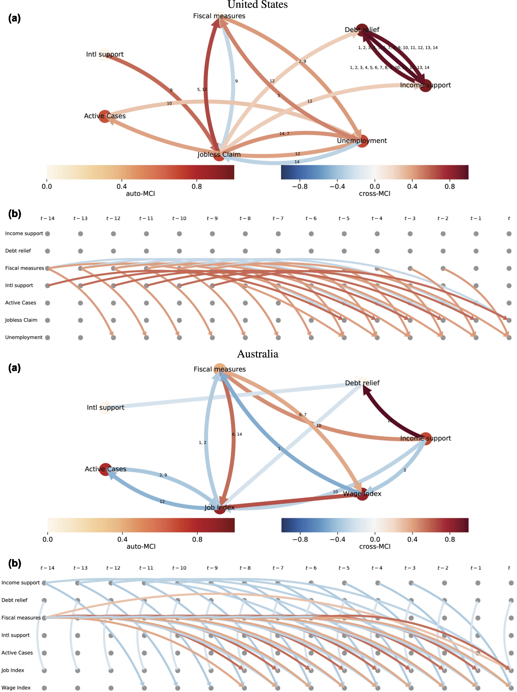
We can see from the Fig. 3 for the United States that “Fiscal Measure” was considered as the cause for a higher number of “Unemployment Rate”. However, as the current COVID-19 pandemic is still spreading in the United States, “Unemployment Rate” is expected to keep going up in the short term, regardless of the fiscal policy. On a brighter note, the blue link indicated that “Fiscal Measure” has some negative impact on the “New Jobless Claim”, which means it helped lower the number of new people who were in need of financial support. “New Jobless Claim” was deemed as the cause for all three domestic economic support. This showed that the United States might have announced these policies after seeing an increasing number of jobless workers. The United States had some basic unemployment insurance programs before the COVID-19 pandemic. In late March, additional income support programs were layered on top of ordinary unemployment insurance. Unemployment insurance in the U.S. is state-specific but overseen by the U.S. Department of Labour. On average, unemployment insurance replaced about 50% of lost wages for a finite period of time. Since the economic and health situation in the United States is not recovered yet, it is still too early to conclude on the effectiveness of these policies.
On the other hand, Fig. 3 for Australia showed that “Fiscal Measures” policies were effective in improving the labour market condition for Australia, with positive red links. Meanwhile, “Income Support” and “Debt Relief” were considered to have a negative causal relationship, worsen the “Job Index” and “Market Index”. This was an expected effect as the “Income Support” policies encourage more people to apply for unemployment benefits, which lessened the number of employed workers and lessen the wage. Since the GDP per capita in Australia was higher than in many other countries [13], the amount of monetary support was also significantly high. A total of 189 billion was being injected into the economy by all arms of Government in order to keep Australians in work and firms in the business. This included 17.6 billion for the Government’s first economic stimulus package on 12/03/2020, 90 billion from the Reserve Bank of Australia and 15 billion from the Government to deliver easier access to finance, and 66.1 billion in the economic support package on 22/03/2020.
Regarding the impact time lags, it took only about 3 days for this causal link to affect the “Wage Index”, while the “Fiscal Measure” took 6 days. However, the colours of these links were also worth noted as the lighter blue indicated a really weak negative impact, and the more positive links had a darker red colour. We can still conclude that monetary and fiscal policies had shown some early positive impacts on the Australian labour market.
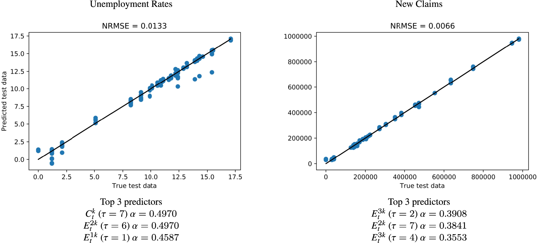
We then used these detected causal links in the training dataset to build the models to forecast the numbers of New Claims and Unemployment Rates in the United States. For both models, we utilised the Gradient Boosting Regressor from Scikit-Learn [21] as the prediction algorithm. The Normalized Root Mean Square Error (NRMSE) reported in Fig. 4 showed that the model prediction accuracy is high. More importantly, we were more interested in explaining the models in terms of evaluating the significant causal links’ suitability as the predictors. As we can see from the results, besides the COVID-19 Active Cases
Fig. 4.
Forecast models for the numbers of unemployment rates (left) and new claims (right) of the United States (testing dataset).
Finally, to test the robustness of these models, we used data from the United States and the Australian labour markets as the sample data to back-test the robustness of our models, using the classical statistics inference approach with Granger Causality. In Table 4, we built statistical models with Granger Causality to back-test the significant causal links of “Fiscal Measures” on the United States and Australian labour markets. All the causal test statistics were significant at a 95% confidence level, which confirms our model results. Moreover, Granger Causality falsely detected links with multiple other time lags (only a few links are randomly reported here). These extra causal links were not considered as significant in the PCMCI model, so we did not have the PCMCI value for false-positive causal links in Table 4.
Table 4
Comparing the causal analysis results of PCMCI and other statistical models using granger causality
| Country | Causal Link | τ | PCMCI | F-test | chi2 test | Likelihood ratio test | Parameter F-test |
| Correct Causal Links detected by PCMCI | |||||||
| United States | 9 | −0.2680 | 12.0963 | 125.4140 | 90.2067 | 12.0963 | |
| 2 | 0.4220 | 16.3985 | 33.9202 | 30.5994 | 16.3985 | ||
| Australia | 6 | 0.5610 | 10.4171 | 68.5664 | 56.2769 | 10.4179 | |
| 6 | 0.3780 | 3.8408 | 25.2804 | 23.3276 | 3.8405 | ||
| False-positive links eliminated by PCMCI | |||||||
| United States | 12 | 8.4178 | 122.7840 | 88.3183 | 8.4178 | ||
| 5 | 6.1948 | 33.4609 | 30.1665 | 6.1945 | |||
| Australia | 11 | 6.7929 | 89.1642 | 69.1968 | 6.7927 | ||
| 13 | 4.5362 | 73.0604 | 58.7907 | 4.5360 | |||
6.Discussion
Through our causal analysis with empirical data from various sources, we have answered our research questions:
Q1: Nations have taken multiple measures amid the COVID-19 pandemic, which can be categorized into three groups: “Containment”, “Health”, and “Economic” policy. Within our group of interests, there are four types of Economic Support policies, namely “Income Support”, “Debt/Contract Relief”, “Fiscal Measures”, and “International Support”. Since the post-pandemic economic fallout will be severe in multiple countries, policymakers should respond with targeted fiscal, monetary, and financial market policies to help impacted workers and organizations locally. On the global scale, multilateral collaboration is vital to recovering from the pandemic, including helping under-developed nations confronting both health and financing crises, especially for countries with weaker health systems. This was not the situation at the beginning of the pandemic as most countries were focusing on their own national problems, which leads to much less international support. As some countries are planning to reopen their borders in the next few months, we are seeing more international aids and cooperation, especially in vaccination and medication support for developing regions.
Q2: Using the combined general indexes of these policies, we analyze the causal relationship of different policy groups to the financial market. From the result in Table 2, we conclude that there are strong causal links observed in many countries. We also confirm that the “Economic Support” policy alone will have less impact on the market than when being combined with other Containment and Health policy. This aligns with previous researches for the GFC as multiple policies are needed at the same time to overcome the crisis. As per our study, some emerging businesses amid the COVID-19 pandemic are healthcare and technology-related, which are affecting the whole financial market on the recovery track. Further analysis of other types of measures, e.g., the impact of investment on vaccines, will reveal some more interesting insights and stimulate more discussions.
Q3: The causal analysis of each type of Economic Support policy on the financial market shows some significant links. “Income Support” tends to be a basic but effective policy in multiple countries. However, “Debt/Contract Relief” and “Fiscal Measure” are quicker to support the financial market prices. As the COVID-19 pandemic has not ended yet, it will be a bit early to have a final conclusion on the effectiveness of these Economic support policies. We believe longitudinal studies using less frequent time series data such as the GDP (per capita) would be essential to confirm the result of this research work. Moreover, in order to accurately assess the impact of the “International Support” policy, we have to further analyze the transnational money flows to see the impact of these aids on the receiving countries, not the giving nations.
Q4: Similarly, it is still a bit early to confirm the effectiveness of the Economic Support policy on the labour market. Still, from our analysis, there are some strong causal relationships observed already with these early data points. Particularly, “Fiscal Measure” is the most impacting policy for both Australia and the United States. Moreover, the market is affected in about 7 days on average, which is better for both salary workers and the fiscal balance of these countries. Once again, when the data is available, a longitudinal analysis using the unemployment rates of all countries will reassert the initial conclusion from this paper.
Last but not least, the forecast models using PCMCI causal links accurately predict the out-of-bag time series of the United States and the Australian labour markets, which might help economists and policymakers in future decisions for better social changes post-pandemic.
7.Conclusion
The COVID-19 pandemic had completely changed the world in 2020, leaving severe damage to all countries around the world, causing both health and financial crises. Governments had been proactive in responding to the pandemic, announcing numerous support policies, in three categories (“Containment”, “Health” and “Economic” policies) on multiple levels for their citizens, local businesses, international organizations, and other nations. From our causal analysis using PCMCI, a graph-based causality search algorithm for multivariate time series, we can see that a combination of all different types of policies might cause a more positive result in more countries.
We analyzed the causal impact of the economic support policies on the financial markets for 80 countries. The results showed that the markets received some early positive effects caused by these policies, reacted in very short time lags, and began to slowly recover from the crisis. “Fiscal Measures” with a big stimulus package was considered to be effective on both the USA and Australian labour markets. Even though more longitudinal studies are required to further confirm the impact of all monetary and fiscal policies amid the COVID-19 pandemic, the initial results from this paper had significantly contributed to the current literature on this topic and can serve as a reference for economists, researchers, policymakers and international organizations.
Notes
Appendices
Appendix
AppendixFinal countries and financial indexes list
In Table 5, we list the chosen 80 financial indexes for 80 countries in our final dataset accordingly.
Table 5
List of countries and financial indexes in the final dataset
| Country | Index | Country | Index | Country | Index |
| Argentina | S&P Merval | Indonesia | IDX Composite | Portugal | PSI 20 |
| Australia | S&P/ASX 200 | Iraq | ISX Main 60 | Qatar | QE General |
| Austria | ATX | Ireland | ISEQ Overall | Romania | BET |
| Bahrain | Bahrain All Share | Israel | TA 35 | Russia | MOEX |
| Bangladesh | DSE 30 | Italy | FTSE MIB | Rwanda | Rwanda All Share |
| Belgium | BEL 20 | Jamaica | JSE Market | Saudi Arabia | Tadawul All Share |
| B&H | BIRS | Japan | Nikkei 225 | Serbia | Belex 15 |
| Botswana | BSE Domestic Company | Jordan | Amman SE General | Singapore | STI Index |
| Brazil | Bovespa | Kazakhstan | KASE | Slovenia | Blue-Chip SBITOP |
| Bulgaria | BSE SOFIX | Kenya | Kenya NSE 20 | South Africa | FTSE/JSE Top 40 |
| Canada | S&P/TSX | Kuwait | FTSE Lujain Kuwait | Spain | IBEX 35 |
| Chile | S&P CLX IPSA | Lebanon | BLOM Stock | Sri Lanka | CSE All-Share |
| China | Shanghai | Malaysia | KLCI | Sweden | OMXS30 |
| Colombia | COLCAP | Mauritius | Semdex | Switzerland | SMI |
| Costa Rica | CR Indice Accionario | Mongolia | MNE Top 20 | Thailand | SET |
| Croatia | CROBEX | Morocco | Moroccan All Shares | Tunisia | Tunindex |
| Cyprus | Cyprus Main Market | Namibia | NSX | Turkey | BIST 100 |
| Denmark | OMXC20 | Netherlands | AEX | Uganda | Uganda All Share |
| Ecuador | Guayaquil Select | New Zealand | NZX 50 | Ukraine | PFTS |
| Egypt | EGX 30 | Niger | NSE 30 | UAE | MSCI UAE |
| Finland | OMX Helsinki 25 | Nigeria | NSE 30 | United Kingdom | FTSE 100 |
| France | CAC 40 | Norway | Oslo OBX | United States | S&P 500 |
| Germany | DAX | Oman | MSM 30 | Venezuela | Bursatil |
| Greece | Athens General Composite | Pakistan | Karachi 100 | Vietnam | VN Index |
| Hungary | Budapest SE | Peru | S&P Lima General | Zambia | LSE All Share |
| Iceland | ICEX Main | Philippines | PSEi Composite | Zimbabwe | Zimbabwe Industrial |
| India | Nifty 50 | Poland | WIG30 |
References
[1] | Y. Ait-Sahalia, J. Andritzky, A. Jobst, S. Nowak and N. Tamirisa, Market response to policy initiatives during the global financial crisis, Journal of International Economics 87: (1) ((2012) ), 162–177. doi:10.1016/j.jinteco.2011.12.001. |
[2] | F. Aslam, S. Aziz, D.K. Nguyen, K.S. Mughal and M. Khan, On the efficiency of foreign exchange markets in times of the COVID-19 pandemic, Technological Forecasting and Social Change 161: ((2020) ), 120261. doi:10.1016/j.techfore.2020.120261. |
[3] | R. Baldwin and E. Tomiura, Thinking ahead about the trade impact of COVID-19. Economics in the Time of COVID-19 59 (2020). |
[4] | T. Bouezmarni, J.V. Rombouts and A. Taamouti, Asymptotic properties of the Bernstein density copula estimator for α-mixing data, Journal of Multivariate Analysis 101: (1) ((2010) ), 1–10. doi:10.1016/j.jmva.2009.02.014. |
[5] | D. Colombo and M.H. Maathuis, Order-independent constraint-based causal structure learning, The Journal of Machine Learning Research 15: (1) ((2014) ), 3741–3782. |
[6] | M.A. Dabrowski, S. Smiech and M. Papiez, Monetary policy options for mitigating the impact of the global financial crisis on emerging market economies, Journal of International Money and Finance 51: ((2015) ), 409–431. doi:10.1016/j.jimonfin.2014.12.006. |
[7] | T. Dergiades, C. Milas and T. Panagiotidis, Effectiveness of Government Policies in Response to the COVID-19 Outbreak, Available at SSRN 3602004 5 (2020). |
[8] | E. Dong, H. Du and L. Gardner, An interactive web-based dashboard to track COVID-19 in real time, The Lancet infectious Diseases 20: (5) ((2020) ), 533–534. doi:10.1016/S1473-3099(20)30120-1. |
[9] | M. Eichler, Causal Inference in Time Series Analysis, Wiley Online Library, (2012) . |
[10] | N. Fernandes, Economic effects of coronavirus outbreak (COVID-19) on the world economy, Available at SSRN 3557504 3 (2020). |
[11] | C.W. Granger, Investigating causal relations by econometric models and cross-spectral methods, Econometrica: Journal of the Econometric Society (1969), 424–438. doi:10.2307/1912791. |
[12] | T. Hale, S. Webster, A. Petherick, T. Phillips and B. Kira Oxford COVID-19 government response tracker. Blavatnik School of Government 25 (2020). Data use policy: Creative Commons Attribution CC, BY standard. |
[13] | IMF. World Economic Outlook Update, January 2021, 2021. |
[14] | M.S. Lall, S. Elekdag and M.H. Alp, Did Korean Monetary Policy Help Soften the Impact of the Global Financial Crisis of 2008–2009? No. 12–15. International Monetary Fund, 2012. |
[15] | S.C. Ludvigson, S. Ma and S. Ng, COVID9 and the macroeconomic effects of costly disasters. Tech. rep., National Bureau of Economic Research, 2020. |
[16] | W.J. McKibbin and R. Fernando, The global macroeconomic impacts of COVID-19: Seven scenarios. |
[17] | W. Mensi, A. Sensoy, X.V. Vo and S.H. Kang, Impact of COVID-19 outbreak on asymmetric multifractality of gold and oil prices, Resources Policy 69: ((2020) ), 101829. doi:10.1016/j.resourpol.2020.101829. |
[18] | M. Nicola, Z. Alsafi, C. Sohrabi, A. Kerwan, A. Al-Jabir, C. Iosifidis, M. Agha and R. Agha, The socio-economic implications of the coronavirus and COVID-19 pandemic: A review, International Journal of Surgery 78: (6) ((2020) ), 185–193. doi:10.1016/j.ijsu.2020.04.018. |
[19] | A. Papana, C. Kyrtsou, D. Kugiumtzis and C. Diks, Simulation study of direct causality measures in multivariate time series, Entropy 15: (7) ((2013) ), 2635–2661. doi:10.3390/e15072635. |
[20] | L. Pastor and P. Veronesi, Uncertainty about government policy and stock prices, The journal of Finance 67: (4) ((2012) ), 1219–1264. doi:10.1111/j.1540-6261.2012.01746.x. |
[21] | F. Pedregosa, G. Varoquaux, A. Gramfort, V. Michel, B. Thirion, O. Grisel, M. Blondel, P. Prettenhofer, R. Weiss, V. Dubourg et al., Scikit-learn: Machine learning in Python, Journal of Machine Learning Research 12: ((2011) ), 2825–2830. |
[22] | S. Ramelli and A.F. Wagner, Feverish stock price reactions to COVID-19, Available at SSRN 3560319 3 (2020). |
[23] | O. Ricci, The impact of monetary policy announcements on the stock price of large European banks during the financial crisis, Journal of Banking & Finance 52: ((2015) ), 245–255. doi:10.1016/j.jbankfin.2014.07.001. |
[24] | J. Runge, Detecting and quantifying causality from time series of complex systems, 2014. |
[25] | J. Runge, P. Nowack, M. Kretschmer, S. Flaxman and D. Sejdinovic, Detecting and quantifying causal associations in large nonlinear time series datasets, Science Advances 5: (11) ((2019) ), eaau4996. doi:10.1126/sciadv.aau4996. |
[26] | C.A. Sims, Money, income, and causality, The American Economic Review 62: (4) ((1972) ), 540–552. |
[27] | P. Spirtes, C.N. Glymour, R. Scheines and D. Heckerman, Causation, Prediction, and Search, MIT Press, (2000) . |
[28] | L. Su and H. White, A nonparametric Hellinger metric test for conditional independence, Econometric Theory 24: (4) ((2008) ), 829–864. doi:10.1017/S0266466608080341. |
[29] | The World Bank. January 2021 Global Economic Prospects, 2021. |
[30] | T. Verma and J. Pearl, Equivalence and Synthesis of Causal Models, UCLA, Computer Science Department, (1991) . |
[31] | R.M. Viner, S.J. Russell, H. Croker, J. Packer, J. Ward, C. Stansfield, O. Mytton, C. Bonell and R. Booy, School closure and management practices during coronavirus outbreaks including COVID-19: A rapid systematic review, The Lancet Child & Adolescent Health 4 5: ((2020) ), 397–404. doi:10.1016/S2352-4642(20)30095-X. |
[32] | C.R. Wells, P. Sah, S.M. Moghadas, A. Pandey, A. Shoukat, Y. Wang, Z. Wang, L.A. Meyers, B.H. Singer and A.P. Galvani, Impact of international travel and border control measures on the global spread of the novel 2019 coronavirus outbreak, Proceedings of the National Academy of Sciences 117: (13) ((2020) ), 7504–7509. doi:10.1073/pnas.2002616117. |
[33] | H. White, Lu and X. Granger, Causality and dynamic structural systems, Journal of Financial Econometrics 8: (2) ((2010) ), 193–243. doi:10.1093/jjfinec/nbq006. |


