
Comparative analysis of supervised learning algorithms for prediction of cardiovascular diseases
Abstract
BACKGROUND:
With the advent of artificial intelligence technology, machine learning algorithms have been widely used in the area of disease prediction.
OBJECTIVE:
Cardiovascular disease (CVD) seriously jeopardizes human health worldwide, thereby needing the establishment of an effective CVD prediction model that can be of great significance for controlling the risk of the disease and safeguarding the physical and mental health of the population.
METHODS:
Considering the UCI heart disease dataset as an example, initially, a single machine learning prediction model was constructed. Subsequently, six methods such as Pearson, chi-squared, RFE and LightGBM were comprehensively used for the feature screening. On the basis of the base classifiers, Soft Voting fusion and Stacking fusion was carried out to build a prediction model for cardiovascular diseases, in order to realize an early warning and disease intervention for high-risk populations. To address the data imbalance problem, the SMOTE method was adopted to process the data set, and the prediction effect of the model was analyzed using multi-dimensional and multi-indicators.
RESULTS:
In the single classifier model, the MLP algorithm performed optimally on the preprocessed heart disease dataset. After feature selection, five features eliminated. The ENSEM_SV algorithm that combines the base classifiers to determine the prediction results by soft voting on the results of the classifiers achieved the optimal value on five metrics such as Accuracy, Jaccard_Score, Hamm_Loss, AUC, etc., and the AUC value reached 0.951. The RF, ET, GBDT, and LGB algorithms were employed in the first stage sub-model composed of base classifiers. The AB algorithm was selected as the second stage model, and the ensemble algorithm ENSEM_ST, obtained by Stacking fusion of the two stages exhibited the best performance on 7 indicators such as Accuracy, Sensitivity, F1_Score, Mathew_Corrcoef, etc., and the AUC reached 0.952. Furthermore, a comparison of the algorithms’ classification effects based on different training set occupancy was carried out. The results indicated that the prediction performance of both the fusion models was better than the single models, and the overall effect of ENSEM_ST fusion was stronger than the ENSEM_SV fusion.
CONCLUSIONS:
The fusion model established in this study improved the overall classification accuracy and stability of the model to a significant extent. It has a good application value in the predictive analysis of CVD diagnosis, and can provide a valuable reference in the disease diagnosis and intervention strategies.
1.Introduction
Cardiovascular disease (CVD), a chronic ailment that significantly impacts global health, has resulted in a staggering number of fatalities in 2016. Statistics indicate that approximately 17.9 million individuals succumbed to cardiovascular disease worldwide, accounting for 31% of all global deaths. Within China, cardiovascular disease ranked as the leading cause of deaths among both the urban and rural residents. In 2019, cardiovascular disease accounted for 46.74% and 44.26% of rural and urban deaths, respectively. These figures increased to 48.00% and 45.86% in 2020. Alarmingly, CVDs have claimed the lives of 2 out of every 5 individuals, with rural areas experiencing higher mortality rates compared to urban areas since 2009. Furthermore, the Chinese hospitals have witnessed a significant number of discharges related to cardiovascular and cerebrovascular diseases in 2020, totaling to 24.28 million cases. This accounted for approximately 15% of the total number of discharges during that period. With the aging population in China, the prevalence of CVDs continues to surge, posing substantial challenges to healthcare investments and resource allocation for the government and the society. Thus, prioritizing effective prevention, diagnosis, and developing treatment strategies for cardiovascular diseases becomes crucial [1]. Given the significance of real-world data, machine learning methods have emerged as valuable tools in generating evidence to support the clinical decision-making and fulfill clinical requirements [2].
Machine learning is a series of algorithms using classification and prediction, which can be classified into supervised and unsupervised learning algorithms based on whether the ending variables are labeled or not. Supervised learning algorithms use the labeled data to train the model, and are used to predict the probability or classification. Some of the widely used supervised algorithms include random forests, support vector machines, and neural networks [3, 4]. Mannil et al. developed a ML model based on the cardiac computed tomography imaging data to predict myocardial infarction, quantified the image data using texture analysis, and used the KNN algorithm to achieve a good performance (sensitivity 69.0%, specificity 85.0%, false positive rate 15.0%, AUC value 0.78) [5]. Arsanjani et al., on the other hand, predicted the hemodialysis reconstruction in patients with suspected coronary artery disease by combining the clinical data and the quantitative image data from myocardial perfusion tomography imaging as features, which were inputted into a Boosting algorithm to achieve a predicted sensitivity of 73.6%
From the above literature, it can be seen that machine learning models have been widely used in CVD prediction, but in terms of the singularity of the model, most of the current classification models for disease prediction are based on a single classifier, and the comparative analysis between classification models is seldom used. Secondly, in terms of the selection of variables in the model, ‘more the better’ is not true for the data of the variables, and medical diagnosis has higher requirements for the accuracy and stability of the models. In terms of model stability, the stability of base classifiers needs to be improvised, while ensemble learning claims to deliver a better prediction performance. In this pursuit, the present study was envisaged to establish a stable and efficient cardiovascular disease prediction model with clinical significance using supervised learning algorithms.
2.Concepts and methods
2.1Random forest
In Bagging, the Random Forest (RF) model [9] is a widely used algorithm. Its main concept is to train multiple decision trees as base classifiers and make predictions through voting in classification problems. Randomness is incorporated in the data and feature selection, resulting in advantages such as high accuracy, generalization ability, reduced overfitting, and robustness against outliers and missing values. To ensure that the base classifiers are independent of each other “as much as possible”, so as to obtain a model with better overall performance, the Random Forest model introduces a greater degree of randomness in the process of creating the forest to correct the ensemble learning model. This leads to utilization of a higher bias in the exchange for lower variance. The specific corrections include: (1) Putative back sampling is performed on the training set, and each decision tree is trained based on a different random subset of the training set. (2) In feature selection, when each decision tree splits nodes, it no longer pursues the best feature among all features, but randomly selects the best feature in the feature subset. With the modified approach of sample sampling and feature sampling, the random forest model offers a greater randomness in creating the forest, which reduces the correlation between the base classifiers, thus improving the overall classification performance of the model.
2.2Multi-Layer Perception
MLP, which stands for Multi-Layer Perception [10], is an artificial neural network that consists of three layers of nodes: an input layer, a hidden layer, and an output layer. Each node in the network is a neuron that utilizes a nonlinear activation function. MLP can recognize complex patterns and relationships in data, especially when the data is not linearly divisible.
2.3K Nearest Neighbors
K Nearest Neighbors (KNN) [11] is an algorithm used for classification and regression tasks. It operates without any parameters and works by associating each sample with its K closest neighboring values. If a majority of the nearest neighbors belong to a specific category, the sample is classified accordingly and shares properties with the samples within that category. This method relies solely on the category of the nearest sample(s) to make classification decisions and determine the category to which a sample belongs. The KNN algorithm focuses on a small number of neighboring samples, while making category decisions. It does not rely on discriminating the class domains or complex methods for category determination. As a result, KNN is particularly suitable for situations where class domains intersect or when there is significant overlap in the sample set. Unlike linear regression and logistic regression, KNN does not involve a loss function, explicit training, or optimization processes. It offers the advantages of being robust to both numerical and discrete data, simplicity, ease of use and understanding, and requires low training time complexity.
2.4Support Vector Machines Classification
The objective of Support Vector Machine Classification (SVM) [12] is to identify the optimal separating hyperplane that maximizes the margin of the training data. In cases where the training data is linearly separable, a linear classifier known as a hard margin support vector machine is learned by maximizing the margin. When the training data is approximately linearly separable, a linear support vector machine known as a soft margin support vector machine is learned by allowing for some misclassifications. In situations where the training data is not linearly separable, a linear support vector machine is learned using kernel methods and soft margin maximization.
2.5Stochastic Gradient Descent
Stochastic Gradient Descent (SGD) [13] is an optimization algorithm commonly used in the machine learning and deep learning to minimize an objective function. It is a variant of the standard gradient descent algorithm, with the main difference being that only one training sample is used for each update of the weights, rather than the entire training set. This has the advantage of being computationally faster, as the amount of computation per iteration is smaller, and also increases the robustness of the algorithm to some extent, as the algorithm is less likely to fall into a local optimum. The basic steps are as follows (1) Initialize the values of
2.6Classification and Regression Tree
Classification and Regression Tree (CART) [14], unlike ID3 algorithm, uses Gini coefficient (Classification Tree) and squared error (Regression Tree) as the basis for the optimal feature delineation, and the complete algorithm includes decision tree pruning in addition to feature selection and segmentation of feature values. CART decision trees utilize the Gini coefficient to classify features, where the Gini value measures the uncertainty of a dataset by indicating the probability of two randomly drawn samples having different categories. Thus, a higher Gini value represents a greater uncertainty in the dataset. CART is applicable for both classification and regression tasks, generating a binary tree structure.
2.7Gradient Boosting Machine
Gradient Boosting Machine (GBM) [15] is a powerful machine learning algorithm commonly utilized for the classification and regression tasks. It employs the concept of “Ensemble Learning” to create a robust learner by combining multiple “weak learners”, typically decision trees. The fundamental principle of Gradient Boosting involves training a new model in each iteration to predict the residuals (the variation between the true value and predicted value) of the previous model. By doing so, each iteration attempts to rectify the errors made by the preceding iteration. Once the training process is completed, the final model is obtained by aggregating all the individual models with appropriate weights.
2.8Light Gradient Boosting Machine
Light Gradient Boosting Machine, referred to as LightGBM [16], is a gradient boosting framework that employs decision trees as base learners. It adopts a Histogram’s decision tree algorithm and Leaf-wise leaf growth strategy, which includes a maximum depth constraint to prevent overfitting, while maintaining high efficiency. LightGBM offers several advantages, including faster training speed, improved efficiency, lower memory usage, better compatibility with large datasets, and provides a support for parallel learning.
2.9XGBoost
XGBoost [17] is an optimized distributed gradient boosting library that aims to be efficient, flexible, and portable. It has achieved high performance in numerous machine learning competitions. XGBoost creates and combines multiple decision trees, automatically handles missing values, and supports various objective functions such as regression, classification, and ranking.
2.10Extremely Randomized Trees Classifier
The Extremely Randomized Trees Classifier (ET) [18] is an ensemble learning technique that combines the results of multiple de-correlated decision trees to produce classification results. Each decision tree in the ensemble is built using a random sample of features from the training data. At each test node, the decision tree selects the best feature from this random sample and splits the data based on a mathematical metric, typically the Gini index. This process of using random samples of features results in the creation of multiple independent decision trees. During the construction of the ensemble, the importance of each feature is determined by calculating the normalized total reduction in the chosen mathematical metric, such as the Gini index.
2.11Adaboost
Adaboost (Adaptive Boosting, AB) [19] is a widely used ensemble learning technique that involves assigning initial weights to the training data and iteratively training multiple weak classifiers. During each iteration, the sample weights are adjusted based on the accuracy of the previous round of classification results. This adjustment increases the weights of the misclassified samples and decreases the weights of correctly classified samples, allowing subsequent weak classifiers to focus more on challenging samples. Each weak classifier is assigned a weight based on its classification accuracy, reflecting its importance in the final classifier. The final strong classifier is constructed by combining all weak classifiers through weighted voting or summation. Through the iterative process of updating sample weights and weak classifier weights, Adaboost continually improves the classification performance, prioritizing the misclassified samples. Ultimately, the Adaboost algorithm yields a robust classifier with high accuracy.
2.12Soft Voting
The main idea of Soft Voting (ENSEM_SV) [20] model follows the principle of majority rule, through the integration of multiple models in order to reduce the variance and improve the robustness of the model. This is done by a comparison of the modeling results of each of the previous seven base models, such as RandomForest, MLP, XGBoost, ET, GBM, LightGBM, and AB that have better results. These models are selected as the primary classifiers to be fused for Voting, with the weight assignments of 5, 1, 1, 1, 3, 1, 2, and 2, and then the predictions of the classifier’s results are determined with the soft-voting method.
2.13Stacking
Stacking algorithm (ENSEM_ST) [21] is used to train multiple base models in the first layer through the initial training set, and then employs the output features of the base models as the input features of the meta-model. Its algorithm is essentially a further generalization of the model. Comparing and analyzing the above models, except for the single logistic regression model, which performs poorly, the four ensemble learning models: RandomForest, ET, GBM, and LightGBM offer superior prediction results without significant differences. Thus, the above four ensemble learning models were chosen to be fused to obtain the sub-models in the first stage. After completing the first stage, we continued to train the data to obtain the four sub-models under the best parameters respectively, and in this process, each sub-model was cross-validated with five folds, so as to avoid the phenomenon of over-fitting. Finally, the Adaboost model was selected as the model of the second stage.
3.Experiment designs
3.1Datasets
The data employed in this study was obtained from the heart disease dataset in the UCI database (http://archive.ics.uci.edu/ml/machine-learning-databases/statlog/heart/heart.data), which contained 1189 samples and 76 attributes. In order to achieve better prediction results, this study pre-processed the original dataset as follows: (1) Redundant attributes and attributes that were not related to heart disease, such as the case code number in the sample data, were eliminated. (2) In order to retain the authenticity of the data, the standardized scores were calculated and the outliers were removed. (3) To address the problem of imbalance of data sample classes in the binary classification problem, resampling was adopted for sample increase, and the Synthetic Minority Oversampling Technique (SMOTE) was utilized to reduce the degree of imbalance between the classes in the dataset to improve the recognition accuracy. After data pre-processing, a final dataset consisting of 1172 sample sizes, 15 independent variables and 1 target variable was obtained. We used the five-fold cross-validation method for model training and prediction. The environment used Windows 7 operating system, and Python software was applied for modeling and analysis.
3.2Evaluation indicators
In order to better verify and compare the effectiveness of each algorithm in the process of data classification, the present study used Accuracy, Precision, Sensitivity, Specificity, F-measure, Log_Loss, Mathew_Corrcoef, Hamm_Loss, Jaccard_Score and AUC value under the ROC curve for comparative analysis [22].
4.Experimental results and analysis
4.1Classification results
In this subsection, a 7:3 ratio was used to divide the data samples into a training set and a test set. A 5-fold cross-validation was used to yeild the optimal value, which was used to train the training set using models such as Random Forest, Multi-Layer Perceptron Machine, LightGBM, etc. Subsequently, the data in the test set was used to make a prediction, and the prediction effect was comparatively analyzed by using the evaluation indexes listed in section 3.2.
Table 1
Classification results of supervised learning algorithms
| Model | RF | MLP | KNN | SVM | SGD | CART | GBDT | LGB |
|---|---|---|---|---|---|---|---|---|
| Accuracy | 0.8409 | 0.8778 | 0.8068 | 0.8267 | 0.8182 | 0.7955 | 0.8153 | 0.7955 |
| Precision | 0.8265 | 0.8691 | 0.8053 | 0.8289 | 0.8529 | 0.8333 | 0.8051 | 0.7947 |
| Sensitivity | 0.8804 | 0.9022 | 0.8315 | 0.8424 | 0.7880 | 0.7609 | 0.8533 | 0.8207 |
| Specificity | 0.7976 | 0.8512 | 0.7798 | 0.8095 | 0.8512 | 0.8333 | 0.7738 | 0.7679 |
| F-measure | 0.8526 | 0.8853 | 0.8182 | 0.8356 | 0.8192 | 0.7955 | 0.8285 | 0.8075 |
| Log_Loss | 5.4949 | 4.2193 | 6.6723 | 5.9855 | 6.2798 | 7.0648 | 6.3780 | 7.0648 |
| Mathew_Corrcoef | 0.6818 | 0.7553 | 0.6126 | 0.6525 | 0.6389 | 0.5942 | 0.6301 | 0.5898 |
| Hamm_Loss | 0.1591 | 0.1222 | 0.1932 | 0.1733 | 0.1818 | 0.2045 | 0.1847 | 0.2045 |
| Jaccard_Score | 0.7251 | 0.7821 | 0.6761 | 0.7046 | 0.6924 | 0.6604 | 0.6879 | 0.6603 |
Figure 1.
Comparison of curves.
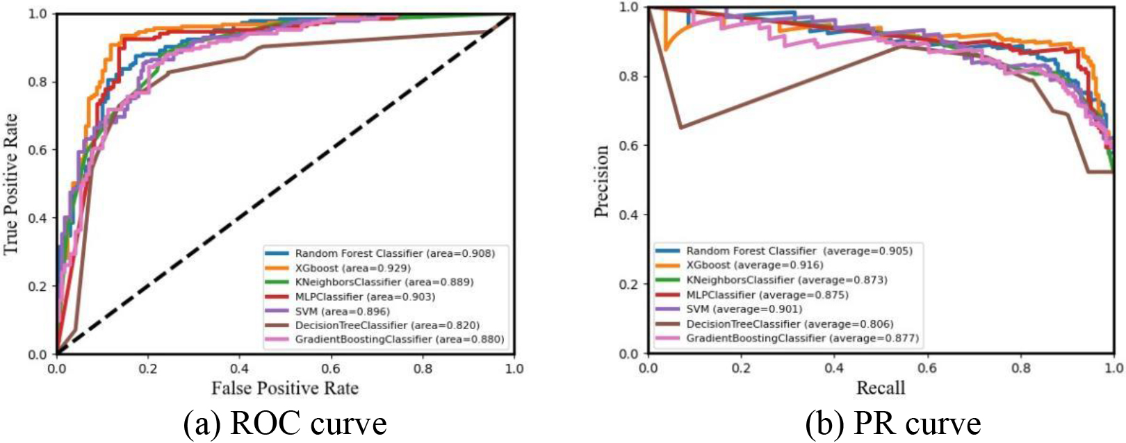
It can be seen from Table 1 and Fig. 1 that the MLP algorithm performed optimally on the pre-processed heart attack dataset with the following parameter settings: solver set to lbfg, learning_rate chosen to be constant, learning_rate_init set to 0.001, maximum number of iterations set to 1,000, random_state to 1, and the
4.2Feature selection
This study addressed the issue of a large number of features in a model that leads to increased size and longer processing times. This can potentially result in overfitting the data and compromising the model’s generalization ability. To improve the interpretability and input quality, we employed various feature selection methods: Pearson correlation coefficient (Pearson), chi-squared metric (chi-squared), recursive feature elimination (RFE), logistic regression (Logistics), impurity-based feature importance in decision trees (RF), and handling of categorical features (LightGBM). The results of these feature selection methods are presented in Table 2. The table shows whether each variable is among the top 10 predictors for each algorithm, indicated by 1 (yes) or 0 (no). The “Total” column represents the number of times a variable was selected by different algorithms.
Table 2
Feature selection results
| Feature | Methods | Total | |||||
|---|---|---|---|---|---|---|---|
| Pearson | Chi-squared | RFE | Logistics | RF | LightGBM | ||
| st_depression | 1 | 1 | 1 | 1 | 1 | 1 | 6 |
| st_slope_flat | 1 | 1 | 1 | 1 | 1 | 0 | 5 |
| max_heart_rate_achieved | 1 | 1 | 1 | 0 | 1 | 1 | 5 |
| exercise_induced_angina | 1 | 1 | 1 | 0 | 1 | 1 | 5 |
| cholesterol | 1 | 0 | 1 | 1 | 1 | 1 | 5 |
| age | 1 | 1 | 1 | 0 | 1 | 1 | 5 |
| st_slope_upsloping | 1 | 1 | 1 | 0 | 1 | 0 | 4 |
| sex_male | 1 | 1 | 1 | 1 | 0 | 0 | 4 |
| chest_pain_type_non-ang_pain | 1 | 1 | 1 | 1 | 0 | 0 | 4 |
| chest_pain_type_atypical_ang | 1 | 1 | 1 | 1 | 0 | 0 | 4 |
| resting_blood_pressure | 0 | 0 | 0 | 0 | 1 | 1 | 2 |
| fasting_blood_sugar | 1 | 1 | 0 | 0 | 0 | 0 | 2 |
| chest_pain_type_typical | 0 | 0 | 1 | 1 | 0 | 0 | 2 |
| rest_ecg_normal | 0 | 1 | 0 | 0 | 0 | 0 | 1 |
| rest_ecg_left | 0 | 0 | 0 | 0 | 0 | 0 | 0 |
4.3Classification results after feature selection
Table 3
Classification results of the algorithm after feature selection
| Model | RF | MLP | KNN | SVM | SGD | CART | GBDT | LGB | ENSEM_SV | ENSEM_ST |
|---|---|---|---|---|---|---|---|---|---|---|
| Accuracy | 0.8438 | 0.8324 | 0.8153 | 0.7869 | 0.8125 | 0.8040 | 0.8097 | 0.8068 | 0.8807 | 0.8807 |
| Precision | 0.8449 | 0.8415 | 0.8940 | 0.7853 | 0.8073 | 0.8443 | 0.7940 | 0.8222 | 0.8817 | 0.8698 |
| Sensitivity | 0.8587 | 0.8370 | 0.7337 | 0.8152 | 0.8424 | 0.7663 | 0.8587 | 0.8043 | 0.8913 | 0.9076 |
| Specificity | 0.8274 | 0.8274 | 0.9048 | 0.7560 | 0.7798 | 0.8452 | 0.7560 | 0.8095 | 0.8690 | 0.8512 |
| F-measure | 0.8518 | 0.8392 | 0.8060 | 0.8000 | 0.8245 | 0.8034 | 0.8251 | 0.8132 | 0.8865 | 0.8883 |
| Log_Loss | 5.3967 | 5.7892 | 6.3779 | 7.3592 | 6.4761 | 6.7704 | 6.5742 | 6.6723 | 4.1212 | 4.1212 |
| Mathew_Corrcoef | 0.6867 | 0.6642 | 0.6443 | 0.5727 | 0.6241 | 0.6117 | 0.6193 | 0.6134 | 0.7608 | 0.7612 |
| Hamm_Loss | 0.1563 | 0.1676 | 0.1847 | 0.2131 | 0.1875 | 0.1960 | 0.1903 | 0.1932 | 0.1193 | 0.1193 |
| Jaccard_Score | 0.7297 | 0.7130 | 0.6872 | 0.6486 | 0.6840 | 0.6722 | 0.6795 | 0.6763 | 0.7868 | 0.7866 |
Figure 2.
Comparison of algorithm curves after feature selection.
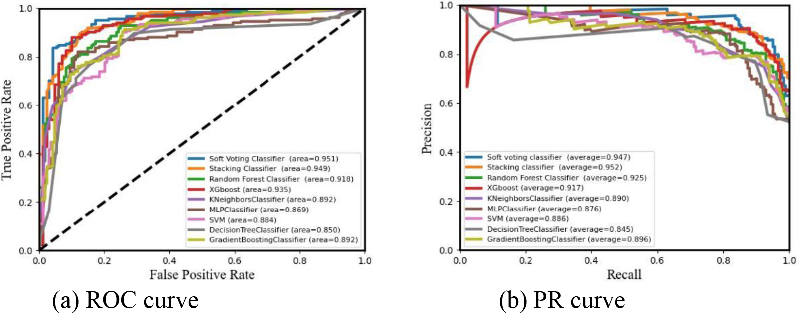
After feature screening, features such as resting_blood_pressure, sex_male, chest_pain_type_non-ang_pain, chest_pain_type_atypical_ang, and rest_ecg_left were eliminated, while introducing the two ensemble learning algorithms: Soft Voting and Stacking. It can be seen from Table 3 and Fig. 2 that the Voting fusion by RF, MLP, XGB, ET, GBDT, LGB and AB algorithms that performed better in section 4.1, was performed according to the weights of 5, 1, 1, 3, 1, 2, 2, and 2, respectively, and the ENSEM_SV algorithm that soft voted the results of the classifiers to determine the prediction results, was used in Accuracy, Jaccard_Score, Hamm_Loss, AUC, etc. The ENSEM_ST was obtained by Stacking fusion of the first-stage sub-model consisting of RF, ET, GBDT and LGB algorithms as base classifiers, and the AB algorithm was selected as the second-stage model that exhibited the best performance in seven metrics such as Accuracy, Sensitivity, F-measure, Mathew_Corrcoef, etc. A best performance was achieved with an area under the PR curve of 0.952. This indicates that the predictive performance of ENSEM_ST model classification was better than the other 9 algorithms, which indicates that model fusion further improved the predictive performance of the model, thereby increasing the robustness, generalization ability, and better prediction for CVD. The
Figure 3.
Comparison of data classification results for 80% training sets.
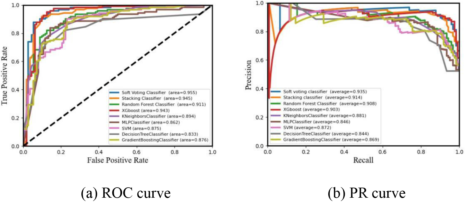
Figure 3 presents the results of the experiments with an 80% share of the training dataset, and with no change in the training method and base classification model parameters. In the context of category imbalance, a large increase in FP can only be exchanged for an insignificant increase in FPR, resulting in the ROC curve presenting an overly optimistic estimate of the effect, and thus the PR curve will outperform the ROC curve when measuring the algorithm’s classification effect. From the area under the ROC curve and the area under the PR curve, the classification effect of Soft Voting and Stacking ensemble learning models was found to be better than other single classification models, with the AUC values of 0.955 and 0.945, respectively, and the AR values of 0.935 and 0.914, respectively, and the Soft Voting model was better than the Stacking model.
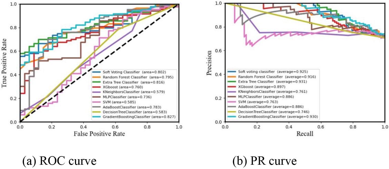
Meanwhile, in order to further validate the effectiveness of the algorithm and increase the comprehensiveness of the algorithmic comparison, this study also conducted supplementary experiments by selecting the Indian Liver Patient Datasets [23] containing 416 liver patient records and 167 non-liver patient records for algorithmic validation, which totaled 10 main attributes, as well as 583 sample sizes. The results of the algorithm comparison are shown in Fig. 4. From the predicted ROC curve and PR curve results, it can be seen that the GBM algorithm and Soft Voting model algorithm achieved better results in binary classification prediction, which may be due to the fact that both are ensemble learning algorithms. Additionally, by two stages of training, the gradual evolution of the set from a weak learner to a strong learner, and a subsequent classification, the overall classification effect was greatly improved.
Figure 4.
Comparison of data classification results for 80% training sets.
5.Conclusions
In the present study, to develop a predictive analysis of CVD diagnosis, we assembled the multiple classes of single classifiers, analyzed and compared the effects of the classifier models under different features, and used the better-performing model as the base classifier. Subsequently, we performed Soft Voting and Stacking model fusion, and comprehensively evaluated the overall performance of each model using multiple assessment metrics, as well as analyzed the important features of the classifiers. Reasonable and efficient use of machine learning models can assist in the high-precision automatic diagnosis and prediction of disease regression, which can help the clinicians in decision-making, save a lot of time and reduce the clinical misdiagnosis rate at the same time. In the future, we will explore the extraction of common risk factors for multiple diseases, realize the joint application of medical clinical data in the prediction of various diseases, and explore the oversampling method for unbalanced data to constrain the algorithm in terms of weights or regular terms. Furthermore, we can direct efforts to improve the accuracy of CVD prediction models by joint parameterization, and develop a visualization and prediction system to monitor and warn patients throughout the life cycle of their visit.
Acknowledgments
This work was sponsored by the Tianjin Health Research Project under Grant No. TJWJ2023QN114 and the In-hospital project of Baodi Clinical College, Tianjin Medical University under Grant No. BDYYQN01.
Conflict of interest
None to report.
References
[1] | Wang SH, Li JJ. Clinical applications of machine learning in cardiovascular diseases. Advances in Cardiovascular Diseases. (2021) ; 42: (2): 144-147. |
[2] | Inoue K, Seeman TE, Horwich T, Budoff MJ, Watson KE. Heterogeneity in the association between the presence of coronary artery calcium and cardiovascular events: A machine-learning approach in the MESA study. Circulation. (2023) ; 147: (2): 132-141. |
[3] | Zhou J, You D, Bai J, Chen X, Wu Y, Wang Z, Tang Y, Zhao Y, Feng G. Machine learning methods in real-world studies of cardiovascular disease. Cardiovascular Innovations and Applications. (2023) ; 7: (1). |
[4] | Bzdok D, Krzywinski M, Altman N. Machine learning: Supervised methods. Nature Methods. (2018) ; 15: (1): 5-6. |
[5] | Mannil M, von Spiczak J, Manka R, Alkadhi H. Texture analysis and machine learning for detecting myocardial infarction in noncontrast low-dose computed tomography: Unveiling the invisible. Investigative Radiology. (2018) ; 53: (6): 338-343. |
[6] | Arsanjani R, Dey D, Khachatryan T, Shalev A, Hayes SW, Fish M, Nakanishi R, Germano G, Berman DS, Slomka P. Prediction of revascularization after myocardial perfusion SPECT by machine learning in a large population. Journal of Nuclear Cardiology. (2015) ; 22: (5): 877-884. |
[7] | Frizzell JD, Li L, Schulte PJ, Yancy CW, Heidenreich PA, Hernandez AF, Bhatt dl, Fonarow GC, Laskey WK. Prediction of 30-day all-cause readmissions in patients hospitalized for heart failure: Comparison of machine learning and other statistical approaches. JAMA Cardiology. (2017) ; 2: (2): 204-209. |
[8] | You J, Guo Y, Kang JJ, Wang HF, Yang M, Feng JF, Yu JT, Cheng W. Development of machine learning-based models to predict 10-year risk of cardiovascular disease: a prospective cohort study. Stroke and Vascular Neurology. (2023) ; svn-2023-002332. |
[9] | Zhang Y, Xiong ZH, Liang ZX, She JC, Ma CC. Structural damage identification system suitable for old arch bridge in rural regions: random forest approach. Computer Modeling in Engineering & Sciences. (2023) ; (7): 447-469. |
[10] | Sheena Smart PD, Thanammal KK, Sujatha SS. An ontology based multilayer perceptron for object detection. Computer Systems Science and Engineering. (2023) ; 44: (3): 2065-2080. |
[11] | Gavagsaz E. Efficient parallel processing of k-nearest neighbor queries by using a centroid-based and hierarchical clustering algorithm. Artificial Intelligence Advances. (2022) ; 4: (1): 26-41. |
[12] | Huang X, Zhang SB, Lin C, Xia JY. Quantum fuzzy support vector machine for binary classification. Computer Systems Science and Engineering. (2023) ; 45: (6): 2783-2794. |
[13] | Luo X, Qin W, Dong A, Sedraoui K, Zhou MC. Efficient and high-quality recommendations via momentum-incorporated parallel stochastic gradient descent-based learning. Automatica Sinica. (2021) ; 8: (2): 402-411. |
[14] | Tung HH, Chen CY, Lin KC, Chou NK, Lee JY, Clinciu DL, Lien RY. Clinciu, Ru-Yu Lien. Classification and regression tree analysis in acute coronary syndrome patients. World Journal of Cardiovascular Diseases. (2012) ; 2: (3): 177-183. |
[15] | Ma HF, Zhao WQ, Zhao YR, He Y. A data-driven oil production prediction method based on the gradient boosting decision tree regression. Computer Modeling in Engineering & Sciences. (2023) ; (3): 1773-1790. |
[16] | Mishra D, Naik B, Nayak J, Nayak J, Souri A, Dash PB, Vimal S. Light gradient boosting machine with optimized hyperparameters for identification of malicious access in IoT network. Digital Communications and Networks. (2023) ; 9: (1): 125-137. |
[17] | Kehili A, Dabbabi K, Cherif A, Fst A. Early Detection of Parkinson’s and Alzheimer’s Diseases Using the VOT_Mean Feature. Engineering, Technology and Applied Science Research. (2021) ; 11: (2): 6912-6918. |
[18] | Soltaninejad M, Yang G, Lambrou T, Allinson N, Jones TL, Barrick TR, Howe FA, Ye X. Automated brain tumour detection and segmentation using superpixel-based extremely randomized trees in FLAIR MRI. International Journal of Computer Assisted Radiology and Surgery. (2017) ; 12: (2): 183-203. |
[19] | Blair B. Automatic characterization of classic choroidal neovascularization by using AdaBoost for supervised learning. Investigative Ophthalmology & Visual Science. (2011) ; 52: (5): 2767. |
[20] | Buyrukolu S. New hybrid data mining model for prediction of Salmonella presence in agricultural waters based on ensemble feature selection and machine learning algorithms. Journal of Food Safety. (2021) . |
[21] | Jahnavi Y, Elango P, Raja SP, Kumar PN. A Novel Ensemble Stacking Classification of Genetic Variations Using Machine Learning Algorithms. International Journal of Image and Graphics. (2023) . |
[22] | Dou Y, Meng W. Comparative analysis of weka-based classification algorithms on medical diagnosis datasets. Technology and Health Care: Official Journal of the European Society for Engineering and Medicine. (2023) ; 31: (S1): 397-408. |
[23] | http://archive.ics.uci.edu/dataset/225/ilpd+indian+liver+patient+dataset. |


