
Potential risk quantification from multiple biological factors via the inverse problem algorithm as an artificial intelligence tool in clinical diagnosis
Abstract
BACKGROUND:
The inverse problem algorithm (IPA) uses mathematical calculations to estimate the expectation value of a specific index according to patient risk factor groups. The contributions of particular risk factors or their cross-interactions can be evaluated and ranked by their importance.
OBJECTIVE:
This paper quantified the potential risks from multiple biological factors by integrated case studies in clinical diagnosis via the IPA technique. Acting as artificial intelligence field component, this technique constructs a quantified expectation value from multiple patients’ biological index series, e.g., the optimal trigger timing for CTA, a particular drug in blood concentration data, the risk for patients with clinical syndromes.
METHODS:
Common biological indices such as age, body surface area, mean artery pressure, and others are treated as risk factors upon their normalization to the range from
RESULTS:
This paper discusses quasi-Newton and Rosenbrock analyses performed via the STATISTICA program to solve the above inverse problem, yielding the specific expectation value in the form of a multiple-term nonlinear semi-empirical equation. The extensive background, including six previous publications of these authors’ team on IPA, was comprehensively re-addressed and scrutinized, focusing on limitations, stumbling blocks, and validity range of the IPA approach as applied to various tasks of preventive medicine. Other key contributions of this study are detailed estimations of the effect of risk factors’ coupling/cross-interactions on the IPA computations and the convergence rate of the derived semi-empirical equation viz. the final constant term.
CONCLUSION:
The main findings and practical recommendations are considered useful for preventive medicine tasks concerning potential risks of patients with various clinical syndromes.
1.Background
This study quantified the potential risk from multiple biological factors by integrating six case studies on clinical diagnosis based on the IPA (inverse problem algorithm) approach. The latter has been widely used in modern research in the last decade due to its unique feature in predicting the biological index from a group of patients’ risk factors, immediately alerting medical doctors to take precautions against acute syndromes. The IPA uses mathematical calculations to estimate the expectation value of a specific index according to patient risk factor groups. Furthermore, the contributions of particular risk factors or their cross-interactions can be evaluated and ranked by their importance [1, 2, 3, 4, 5, 6]. Unlike the Taguchi optimization algorithm, which is used to optimize one purpose from a combination of multiple factors [7, 8, 9, 10], IPA directly estimates the expectation value from a group of data. Thus, IPA provides more quantified information than Taguchi’s approach, suggesting just the optimal combination of factors.
A practical application of IPA usually starts from the expectation value definition, which can be the concentration of a particular drug in the patient’s blood [3], the severity of coronary artery [2], carotid stenosis [4], or even the optimal CTA timing for head and neck scanning [5, 6] as well. The IPA is operated according to numerous data of the patient’s biological index. Thus, the precise estimation of expectation value is made by the numerical analysis of a specific inverse matrix. The rank of the original data matrix can be defined as [N
Six IPA-related research topics are evaluated in this study. Each study used five, six, or seven biological indices, and the adopted patients’ number varied from 100 to 1001. In the overview of the IPA technique, we provided a flowchart to illustrate the general idea of how researchers apply IPA in application of artificial intelligence and how to convert the risk factor into dimensionless numerical digits with the normalization process. In the discussion section, we elaborate on the outcomes of the STATISTICA program, interpret risk factors’ cross-interactions, and discuss the IPA procedure’s convergence.
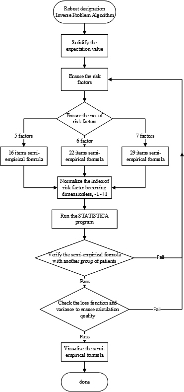
Figure 1.
The flowchart of specific workload illustrating how researchers apply the IPA technique in application of artificial intelligence.
2.An overview of IPA
2.1IPA flowchart
Figure 1 illustrates the flowchart of IPA operation in application of artificial intelligence. As depicted, the quantified expectation value of the project must be defined first, and then the number of risk factors should be preset. Noteworthy is that the adopted factors have to maintain their orthogonality to each other. In addition, the estimated expectation value must be verified through another group of patients’ data to ensure its accuracy. Any failure in verifying or checking the program outcomes (loss function, variance, or correlation coefficient) from STATISTICA necessitates to go back to the preliminary stage in re-defining the risk factors or increasing the number of patients’ data because the program may not converge to an acceptable range due to the limited data scope.
2.2Assigning the essential risk factors
The semi-empirical formula, as recommended by IPA, includes five to seven individual factors that cannot be derived from each other. For instance, weight and body mass index (BMI) cannot be assigned as two independent factors in one study since BMI can be derived from the patient’s weight and height W/H
2.3Defining the semi-empirical formula
Multiple terms are also fixed once the number of risk factors is determined. The semi-empirical formula contains only contributions from the factor and the cross-interactions between two factors. Therefore, neither triple (
(1)
(2)
(3)
The coefficient matrix [
First assume that in a linear equation
(4)
(5)
Assuming that
(6)
(7)
(8)
(9)
Here the dataset matrix-vector is
2.4Normalization of risk factors
Each risk factor must be normalized to become dimensionless before its input into the STATISTICA program. This ensures that the contribution from each factor can be equally dealt with although technically the program can be run without normalization. Each risk factor needs to be converted into the same range between
(10)
As denoted, the
2.5Running the STATISTICA default program
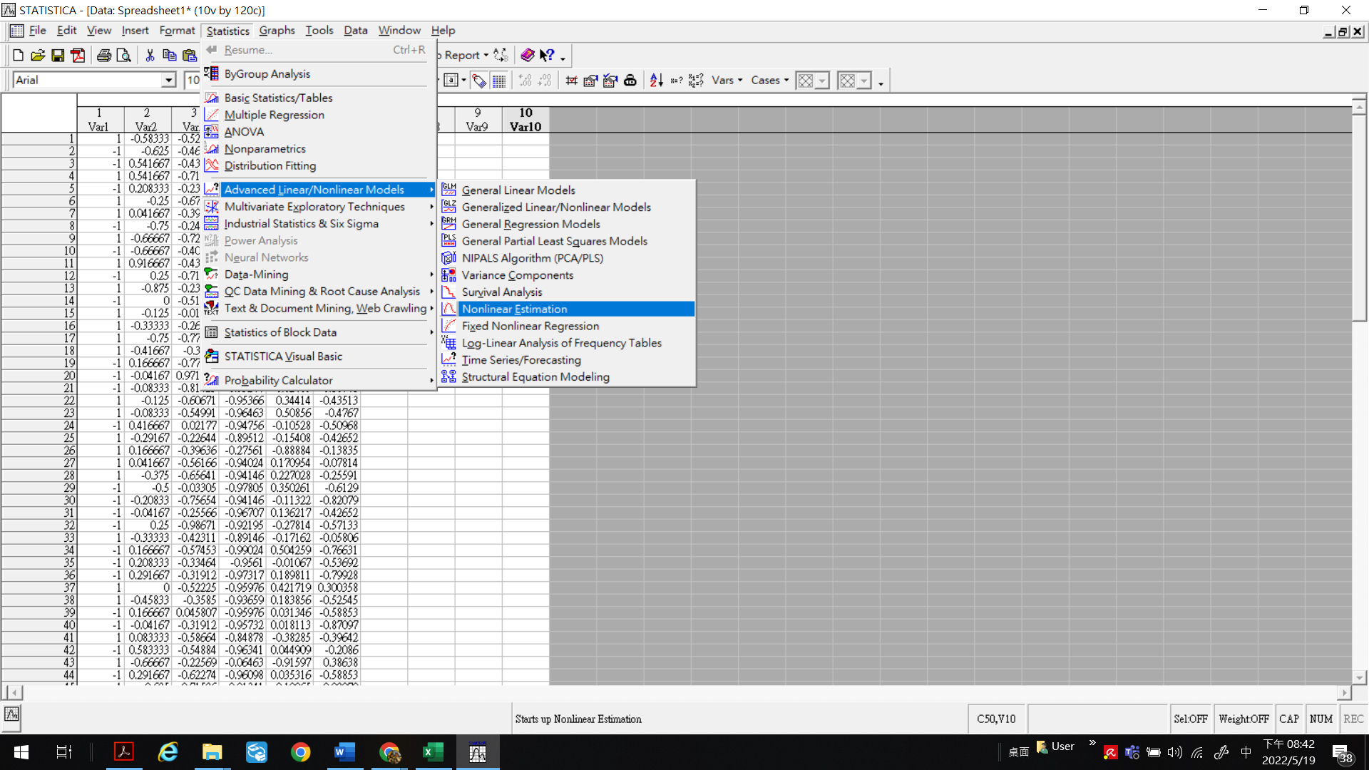
STATISTICA 7.1 version [14] was run to realize the inverse program algorithm, yielding the kernel function [14]. Correlations and cross-interactions among the risk factors were analyzed via user-defined regressions and first-order nonlinear models. Data from the primary group of specific patients were normalized and fed into the numerical tests for the loss function customization. Alternatively, Simplex or Rosenbrock pattern search techniques could yield converged solutions for these loss functions, while deriving the minimum loss function necessitated involving the Rosenbrock or quasi-Newton integrated approaches. Figure 2 depicts a typical STATISTICA program in function. The user needs to follow the suggested option and define the unique loss function to obtain the coefficients’ matrix according to the IPA technique. The STATISTICA program is fully compatible with EXCEL, so the original data can be calculated and arranged in EXCEL and then copied to STATISTICA for further analysis to save the processing time.
Figure 2.
A typical STATISTICA program in function. The user needs to follow the suggested option and define the unique loss function to obtain the coefficients matrix according to the IPA technique.
3.Integrated review of the IPA technique
3.1Integrated study of quantified prediction of expectation
Table 1
Six IPA- related papers were integrated and evaluated in this study. The following acronyms were used: BSA is body surface area, BUN is blood urea nitrogen level, CRP is C-reactive protein, CTA-TT is the suitable triggered timing of computer tomography angiography, CMS is contrast media solution, CMD is contrast media dosage, LDL-C is low-density lipoprotein-cholesterol, LRA/US is the maximal ratio of both left-and-right-arterial-to-upper sinuses, and Pre is the specific pressure of the injector for CMD
| References | ||||||
|---|---|---|---|---|---|---|
| [1] | [2] | [3] | [4] | [5] | [6] | |
| Expectation value | Serum creatinine after administering CMS | Coronary artery stenosis | Digoxin reading | Carotid stenosis | LRA/US | CTA-TT |
| Risk factor | BSA | Age | BSA | Age | CTA-TT | Age |
| Administered CMS | BSA | BUN | LDL-C | MAP | MAP | |
| Serum creatinine before administering CMS | MAP | Creatinine | MAP | Heart rate | HR | |
| BUN | Sugar AC | Na ions | Sugar AC | CMS | CMD | |
| Systolic blood pressure | LDL-C | K ions | CRP | Pre | Pre | |
| Mg ions | BSA | BSA | ||||
| MAP | ||||||
| Original patient’s number | 70 | 93 | 168 | 217 | 216 | 802 |
| Verified patient’s number | 30 | 45 | 45 | 55 | 35 | 199 |
| Loss function | 0.235 | 3.589 | 2.175 | 2.3543 | 2.0144 | 4.4084 |
| 0.9855 | 0.7955 | 0.8920 | 0.8746 | 0.9313 | 0.8965 | |
| 0.986 | 0.795 | 0.892 | 0.875 | 0.931 | 0.897 | |
Table 1 shows the integrated evaluation of the IPA-related papers. As depicted, the expectation value may be the serum creatinine index after contrast administration for the patient with cardiac diagnosis [1] or digoxin reading after the patient was administered digoxin [3]. Nevertheless, the expectation values in the same study could be either the maximal ratio of both left-and-right-arterial-to-upper sinuses (LRA/US) or suitable triggered timing of computer tomography angiography (CTA-TT) [5, 6]. Yet, the preliminary study of LRA/US helps to confirm the correlation among CTA-TT with other risk factors. Thus, a large group of patients was recommended to collect the data for further analysis of CTA-TT in the follow-up study. Eventually, the derived semi-empirical formula can provide instant estimation for patients who have undergone CTA examination. Most risk factors are biological indices collected in routine examination, such as Age, BSA, Sugar AC, or MAP. The number of patients for further verification is strongly suggested as 1/5 to the original patient’s number to create the database of STATISTICA 7.1. The loss function is defined as (OBS-PRED)
Figure 3.
(A) A
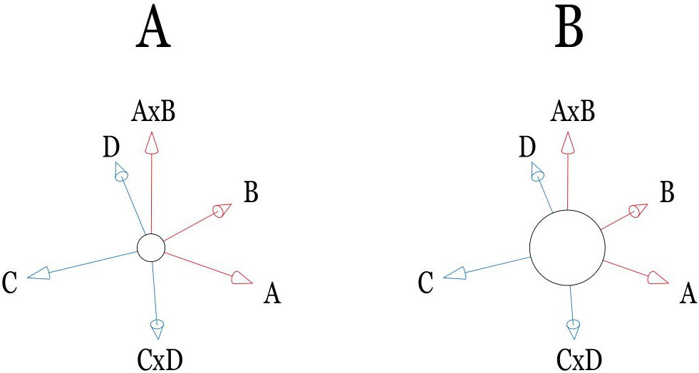
Figure 4.
The mathematical phenomena of convergence in IPA technique presumption. If the large constant dominates the IPA performance, the compromised solution series may rapidly damp to a stable position. Otherwise, it takes a long computational time to converge.
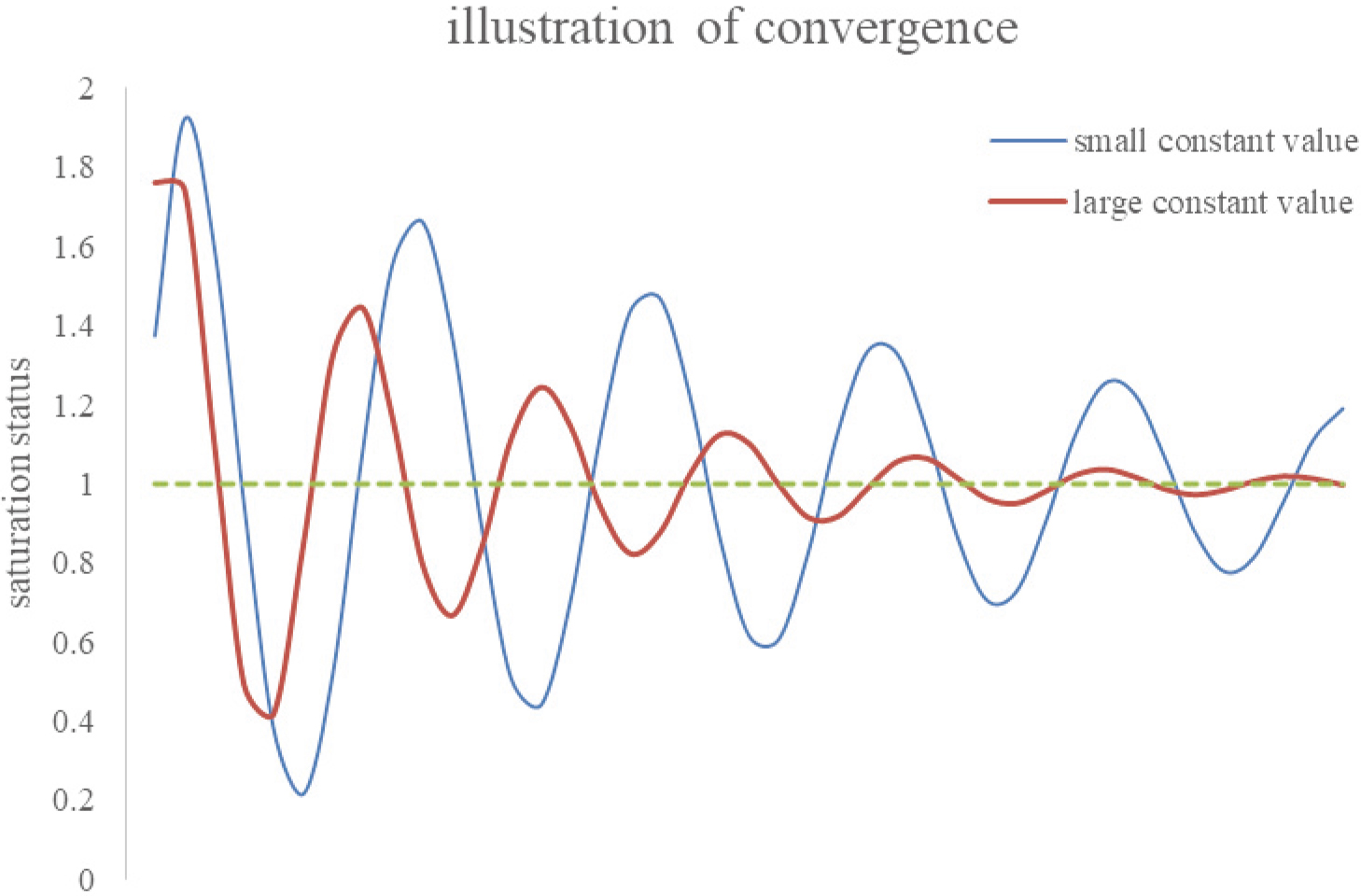
Figure 5.
(A) The X-, Y-, and Z-axes represent BSA (1.19
3.2Interpretation of coefficients of risk factors
The obtained coefficients of risk factors from STATISTICA running imply the importance of the specific risk factor. The personal biological examination’s original data of risk factors are normalized to eliminate their dimensionality. Therefore, Age, BSA, MAP, and all other factors’ data become converted into integer values between
3.3Cross-interactions among factors
In some special cases, the individual factor may not offer a dominant contribution to the expectation value. In contrast, cross-interactions among factors can strongly dominate the performing. According to IPA computational presumption, the cross-interaction between two factors (A and B) can be interpreted as A
3.4The IPA prediction convergence
A sizeable constant term in the semi-empirical formula is always preferable in the IPA predictions. Although it reduces the accuracy of estimation, it indicates the system stability in pursuing a compromised solution via numerical analysis. As illustrated in Fig. 3B, a constant term in the semi-empirical formula can be treated as the average expectation value of all individual patients. In contrast, contributions of other terms in the formula are either dominant (terms with large coefficients) or minor (terms with small ones) respectively to the outcome. Specifically, Fig. 3A shows a comparatively small constant value. In other words, other large coefficients might dominate the formula’s performance and cause more time to optimize the compromised solution. Figure 4 interprets the mathematical phenomena of convergence in IPA presumption. Once a large constant dominates the IPA performance, the compromised solution series may rapidly damp to a stable value. Otherwise, a long computational time is required for its convergence. However, a large constant also indicates a minor alignment that can be achieved in optimizing the solution. Noteworthy is that only in the study of Pan et al. [1], the rank of constant (rank 14/16) was less than any others, namely, ranks 6/16, 7/29, 5/16, 5/22, and 6/22, respectively in the studies [2, 3, 4, 5, 6]. Thus, the optimized loss function,
3.5The application of IPA in preventive medicine
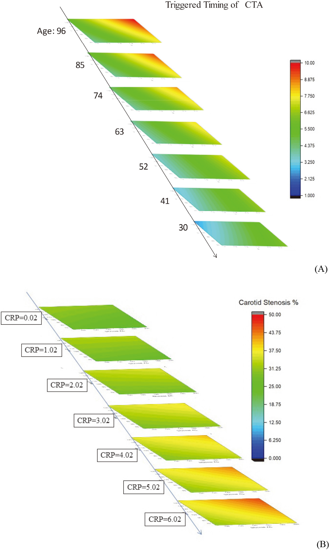
A simple visualization of the IPA technique prospects in preventive medicine can be obtaining by plotting the IPA calculated outcomes via a ladder diagram [4, 6]. In doing so, three dominant risks are assigned as X-, Y-, and Z-axis, respectively. The other risk factor is set as 0.0 after normalization because 0.0 implies an average value of that specific factor (cf. Eq. (10)). Thus, the preset scenario describes a general case of patients. Figure 5, (A) presents IPA-based timing optimization of head and neck CTA for 1001 patients in 2020–2021, whereas the respective ladder diagram represents BSA (from 1.19 to 2.36 m
4.Conclusions
This paper re-addressed and integrated six previous studies of these authors, focusing on the validity range and stumbling blocks of the inverse problem algorithm implementation into artificial intelligence and computer-aided medical applications. The integral part of this technique’s practical realization was normalizing several risk factors’ indices, thus eliminating their various dimensionalities and yielding a quantified integer data interval from
Acknowledgments
This study was financially supported by the Taichung Armed Forces General Hospital, Taiwan (Contract no. TCAFGH-D-111037).
Conflict of interest
None to report.
References
[1] | Pan LF, Davaa O, Chen CY, Pan LK. Quantitative evaluation of contrast-induced-nephropathy in vascular post-angiography patients: Feasibility study of a semi-empirical model. Bio-Medical Materials and Engineering. (2015) ; 26: : s851-860. |
[2] | Pan LF, Chiu SW, Xiao MF, Chen CH, Pan LK. Revised inverse problem algorithm-based prediction of coronary artery stenosis readings from the clinical data of patients with coronary heart diseases. Computer Assisted Surgery. (2017) ; 22: (s1): 70-78. |
[3] | Lin YH, Hsiao KY, Chang YT, Kittipayak S, Pan LF, Pan LK. Assessment of effective blood concentration readings from clinical data on patients with heart failure diseases after digoxin intake: A projection based on the inverse problem algorithm. JMMB. (2019) ; 19: (8): 1940061. |
[4] | Lin YH, Chiu SW, Lin YC, Lin CC, Pan LK. Inverse problem algorithm application to semi-quantitative analysis of 272 patients with ischemic stroke symptoms: Carotid stenosis risk assessment for five risk factors. JMMB. (2020) ; 20: (9): 2040021. |
[5] | Lin CS, Chen YF, Deng J, Yang DH, Pan LF, Pan LK. A six-parameter semi-quantitative analysis of 251 patients for the enhanced triggered timing of head and neck CT angiography scanning via the inverse problem algorithm. JMMB. (2020) ; 20: (10): 2040045. |
[6] | Liang CC, Pan LF, Chen MH, Deng J, Yang DH, Lin CS, Pan LK. Timing optimization of head and neck CT angiography via the inverse problem algorithm: In-vivo survey for 1001 patients in 2020–2021. JMMB. (2021) ; 21: (10): 2140055. |
[7] | Lin CS, Chen YF, Deng J, Yang DH, Chen MH, Lin YH, Pan LK. Taguchi-based optimization of head and neck CT angiography: In-vivo enhanced triggered timing for 600 patients. JMMB. (2021) ; 21: (9): 2140041. |
[8] | Chiang CY, Chen YH, Pan LF, Cho CC, Peng BR, Pan LK. The minimum detectable difference of C.T. angiography scans at various cardiac beats: Evaluation via a customized oblique V-shaped line gauge and PMMA phantom. JMMB. (2021) ; 21: (10): 2140066. |
[9] | Pan LF, Chen YH, Wang CC, Peng BR, Kittipayak S, Pan LK. Optimizing cardiac C.T. angiography minimum detectable difference via Taguchi’s dynamic algorithm, a V-shaped line gauge, and three PMMA phantoms. THC. (2022) ; 30: (S1): 91-103. |
[10] | Ke CH, Liu WJ, Peng BR, Pan LF, Pan LK. Optimizing the minimum detectable difference of gamma camera SPECT images via the Taguchi analysis: A feasibility study with a V-shaped slit gauge. Applied Sciences. (2022) ; 12: : 2708. |
[11] | Huang W, Gallivan KA, Absil PA. A Broyden class of quasi-Newton methods for Riemannian optimization. SIAM J. OPTIM. (2015) ; 25: (3): 1660-1685. |
[12] | Luan VT, Ostermann A. Exponential Rosenbrock methods of order five construction, analysis and numerical comparisons. Journal of Computational and Applied Mathematics. (2014) ; 255: : 417-431. |
[13] | Sesso HD, Stampfer MJ, Rosner B, et al. Systolic and diastolic blood pressure, pulse pressure, and mean arterial pressure as predictors of cardiovascular disease risk in men. Hypertension. (2000) ; 36: : 801-807. |
[14] | STATISTICA version 7.1.30.0, http://www.statsoft.com. |
[15] | Kreyszig E. Advanced Engineering Mathematics, 10ed. Wiley Co. Ld., USA. 2011 ISBN: 0470646136. |


