
A theoretical framework of gradient coil designed to mitigate eddy currents for a permanent magnet MRI system
Abstract
BACKGROUND:
High installation and operating cost have limited applications for many circumstances. In practice, primary and shielding coils cannot insert into the magnet pole simultaneously owing to deficient workspace for the planar permanent MRI systems
OBJECTIVE:
To minimize eddy currents induced in the resist-eddy current plates and pole piece when the gradient coil current switches on and off rapidly.
METHODS:
A theoretical framework that have minimum power dispassion and magnetic energy with eddy plate is proposed for a planar gradient coil. The mirror image of the magnetostatic model is substituted into the stream function for designing a minimum power dispassion planar gradient coil. A finite-difference is used to formulate the coil distribution that makes magnetic field similar to the required magnetic field for gradient coil design.
RESULTS:
A coil designed with actively shielded was simulated and compared with the designed gradient coils using mirror image theory and piece pole effect. According to the numerical evaluation of the x and z coils, the operating currents in the cases were reduced to 34.4% using magnetostatic mirror-image method to replay the active shielding. Moreover, there was a significant improvement on the shielding effect when added to resistive eddy current plate.
CONCLUSIONS:
Using the magnetostatic mirror image theory and mirror-image model, the current density function that could not only gives the minimum power dissipation and magnetic energy with the presence of the eddy plate and pole piece effect, but also provides excellent coil performance compared with active shielding solution.
1.Introduction
For modern medical application, superconducting magnetic resonance imaging (MRI) system has been a powerful medicine device, especially in noninvasive imaging modality aspect compared with computed tomography (CT) and x-ray technology [1]. Gradient coils, as a vital component of an MRI system, are usually designed to provide a linear and orthogonal gradient field along the three axes to spatially encode the information of tissue [2, 3]. Gradient coil that using passive shield technology cannot prevent eddy currents on the surrounding conductors when the current switching quickly, which may lead to serious image distortion [4, 5], energy loss [6], mechanical vibration [7], and eddy artifact [8]. Comparatively, active masking technology has a better image and lower noise caused by eddy currents than passive shielded coils, which is widely used in the MRI systems.
However, high installation and operating cost have limited applications for many circumstances. In practice, primary and shielding coils cannot insert into the magnet pole simultaneously owing to deficient workspace for the planar permanent MRI systems [9]. In order to reduce the eddy current and improve magnetic field quality to get a better image result, more and more coil design methods were discussed in MRI systems. Generally, there are two different kinds of design philosophy. Pre-emphasis is frequently used method, e.g., gradient waveform alternation by providing extra current to compensate for the second magnetic field affected by eddy currents. Alternatively, different types of shielding method also can be used for preventing eddy currents. For the actively shielded method, the current direction reverses in the primary coil and shielding coil layers so that so that the magnetic flux beyond the gradient coil can be offset largely [10]. Passively shielded method is often implemented outside of the gradient coils by applying a certain thickness metallic cylinder or plate [11]. In order to reduce the eddy current and improve magnetic field quality, high permeability materials is used to insert between the magnet and coil layers to enhance the low-frequency shielding performance. However, the hysteresis characteristics is difficult to eliminate so that magnetic field propagates through the multi-cylinder cryostat vessel in the low frequency. For example, Moon proposed a minimum inductance coil design method around the gradient coil [12]. Zu et al. presented analytical expressions for the magnetic field by multilayer dielectric plane and line current model [13].
In this paper, at theoretical gradient coil design approach using mirror-image theory was proposed for planar permanent MRI system. The proposed gradient coils considered the mirror-current around the magnet pole and resist-eddy current plate, which offered sufficient magnet space for patient and MRI system components, such as cooling devices. In the gradient coil design procedure, the power dissipation, stored energy, and field linearity were optimized to achieve the designed gradient fields. For a better comparison, a set of counterpart coil with same dimension and parameter using actively shielded method were simulated.
2.Method
In this section, a mirror image concept was adopted to design the planar gradient coil [14]. A resistive eddy current plate model was incorporated to replace the shielding coils and cause a limitation on eddy currents in the permanent magnet MRI device. The gradient coil optimization was achieved using a stream function-combined finite difference method.
Figure 1.
The planar MRI configurations showing limited space is available for the gradient assembly.
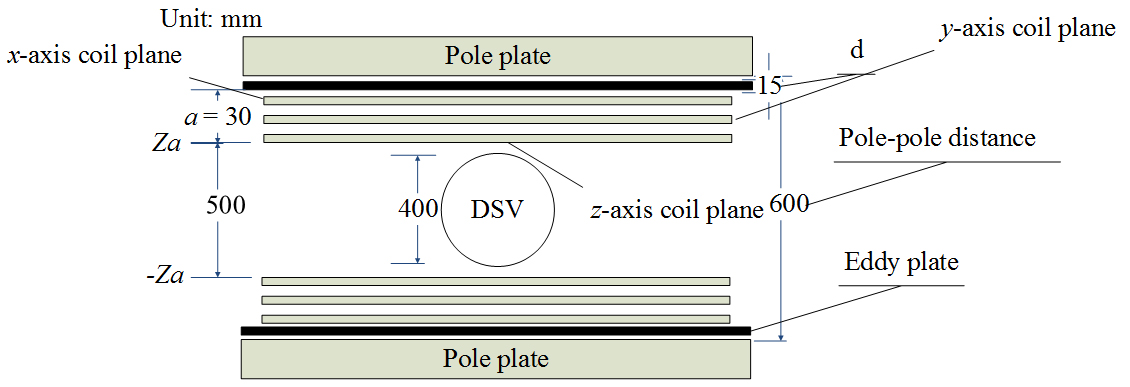
2.1Planar coil geometry and property
As shown in Fig. 1, only 50 mm space (in the z-direction) is available for installing the gradient coils in the planar MRI system. In practice, six active shielded coil layers (x, y and z) is impossible to place the limited space. In this paper, a whole resist-eddy current (thickness: d) is adopted to replace set of shielded gradient coils, offering a magnetic gradient field and a beter-shielding effect. Figure 1 presents the principle scheme coil layer dimensions. The three “plates” are x-axes coil, y-axes coil and z-axes coil respectively. In Fig. 1, the MRI system includes two magnet poles sited in top and bottom, a presents the distance between the coil layer (
2.2Mirror-image theory combined finite-difference method
In a vacuum space, the magnetic field generated by a current source could be calculated following Biot-Savart law. However, the effects of the magnetization current should be considered if there is a ferromagnetic medium nearby [15]. A whole resist-eddy current plate (thickness: d) can be divided into three regions, two boundaries are produced in the process, namely interface 1 and interface 2 (see the Fig. 2). As illustrated in Fig. 2, magnetic medium (relative permeability
Figure 2.
Three-layer region for the resist-eddy current plate (below coil plane
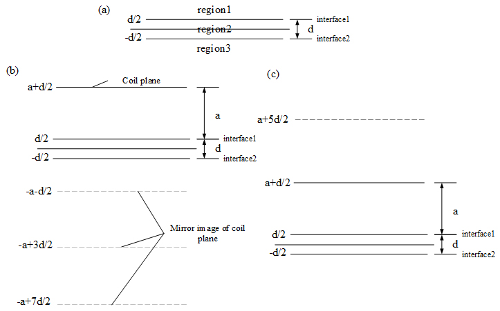
In this work, a pair of resist eddy current plate was added to prevent the eddy current in the magnet pole. The coil layers located at
(1)
Based on the mirror-image theory and Ampere loop theorem under medium/boundary condition, the locations and amplitudes of the mirror current were calculated as follows [13]:
(2)
(3)
where
(4)
where the superscripts
A finite difference method (FDM) was employed to improve the gradient coil design [16, 17]. In the continuity equation of current density,
(5)
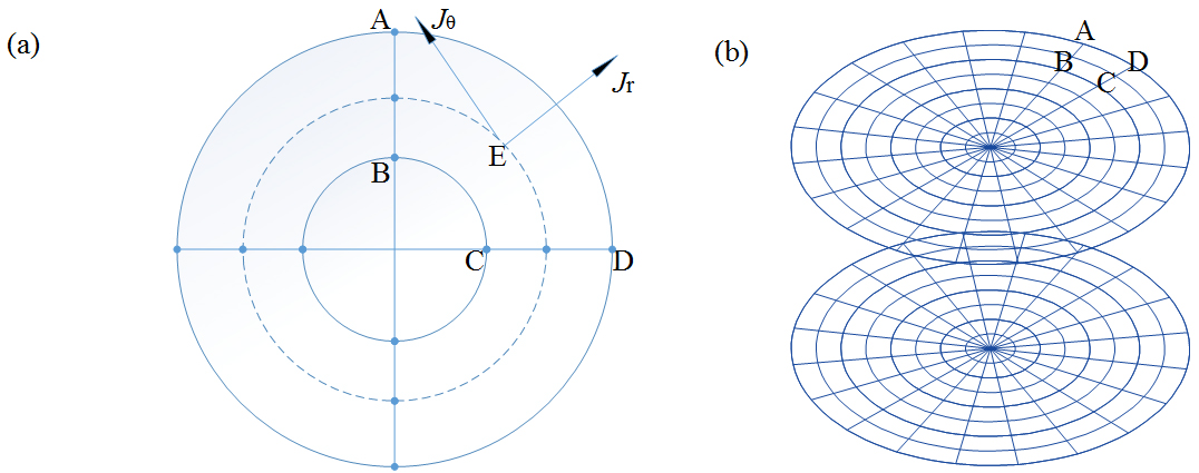
In the Fig. 3, the biplanar gradient coils discretization have been divided two directions, radial and circumferential directions respectively (see the Fig. 3a). For the biplanar coil surface the current density components can be approximated as follows:
(6)
According to the Biot-Savart law, the z-component of magnetic field in DSV region is defined as [20]:
(7)
where
(8)
(9)
Assuming that the contour level that is equally spaced is set as Nc, then we obtain
Figure 3.
Biplanar coil surface’s discretization using FED mesh. (a) radial and circumferential components of current density, (b) the planar gradient coil mesh.
2.3Optimization method of the gradient coil design
To obtain the coil optimization performance , an objective function was proposed related to linearity of magnetic field, power dissipation and magnetic energy in this part. The stored magnetic energy and power dissipation can be written respectively as [21, 22]:
(10)
(11)
where
(12)
where
(13)
where Ais the matrix format refer to the current density source and target field region;
(14)
where
Table 1
Coil geometry and characteristics
| Items | Parameter | Case I-1 | Case I-2 | Case II-1 | Case II-2 | Case III | Case IV |
| Resist eddy | Radius (m) | 0.45 | 0.45 | 0.45 | 0.45 | ||
| current | Thickness (mm) | 15 | 15 | 15 | 15 | ||
| plate | Relative permeability | 440 | 1616 | 440 | 1616 | ||
| Gradient | Radius (m) | 0.43 | 0.43 | 0.43 | 0.43 | 0.43 | 0.43 ( |
| coil | 0.48( | ||||||
| Distance between above and below plane (m) | 0.25 | 0.25 | 0.25 | 0.25 | 0.25 | 0.25 | |
| Wire width (mm) | 3 | 3 | 3 | 3 | 3 | 3 | |
| Wire thickness (mm) | 3 | 3 | 3 | 3 | 3 | 3 | |
| Pole plate | Relative permeability | 4000 | 4000 | ||||
| Thickness (mm) | 30 | 30 | |||||
| Target field | Field strength (mT/m) | 24 | 24 | 24 | 24 | 24 | 24 |
| DSV (m) | 0.4 | 0.4 | 0.4 | 0.4 | 0.4 | 0.4 |
3.Results and discussion
In all different kinds of MRI, magnetic-field component is required to vary linearly along three directions in the z axis. Its linearity is a crucial indicator of the gradient coil quality defined as:
(15)
where
Table 2
The comparison of the biplanar unshielded/shielded gradient coil and proposed coil using a mirror image of the magnetostatic method
| Properties | Case I-1 | Case I-2 | Case II-1 | Case II-2 | Case III | Case IV |
|---|---|---|---|---|---|---|
| Number of Loops (P/S) | 40/NA | 40/NA | 40/NA | 40/NA | 44/NA | 44/32 |
| Current amplitude (A) | 321.25 | 319 | 324.24 | 323.35 | 341.57 | 521.48 |
| Maximum field error (%) | 5.07 | 5.08 | 5.06 | 5.06 | 5.15 | 5.08 |
| Inductance ( | 188.85 | 189.1 | 180.90 | 180.50 | 170.43 | 475.31 |
| Resistance (m | 165.23 | 165.32 | 171.17 | 171.40 | 153.86 | 305.07 |
| Efficiency | 74.70 | 75.23 | 74.01 | 74.22 | 70.26 | 46.02 |
| FoM, | 2.95 | 2.93 | 3.03 | 3.05 | 1.03 | 1.24 |
| 3.38 | 3.42 | 3.20 | 3.21 | 1.62 | 1.37 | |
| Minimum wire spacing (mm) | 4.8 | 4.8 | 4.8 | 4.8 | 5.2 | 5.2 |
Figure 4.
Designed passively shielded and actively shielded
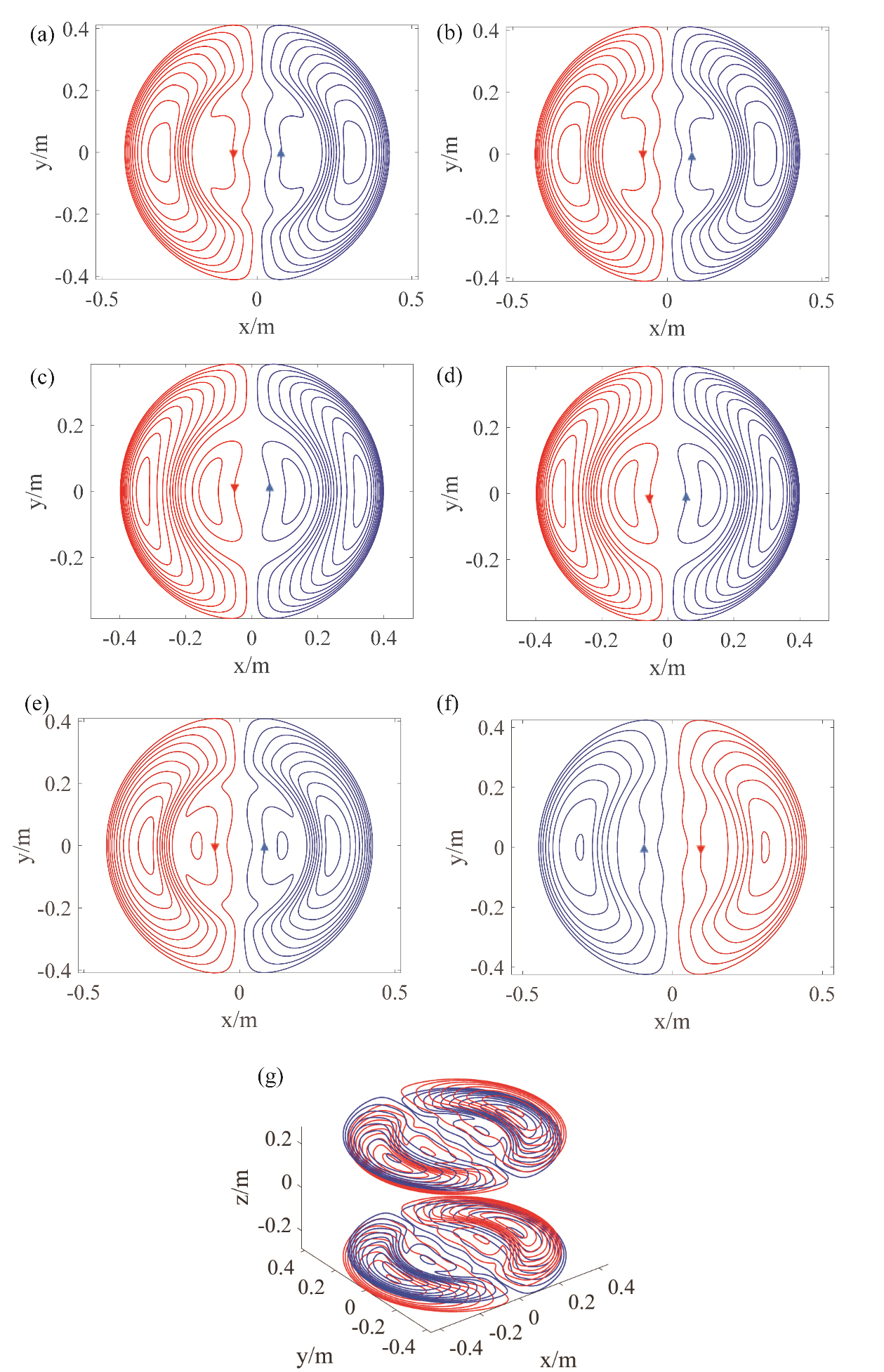
Figure 4 shows the coil winding patterns with same function contour of x-transverse coil. To demonstrate the coil configuration clarify, different kinds of coil patterns were plotted, where Fig. 4a and b presents the coil patterns generated using mirror-image theory with different materials
Figure 5.
Magnetic field distribution for the shielded and unshielded
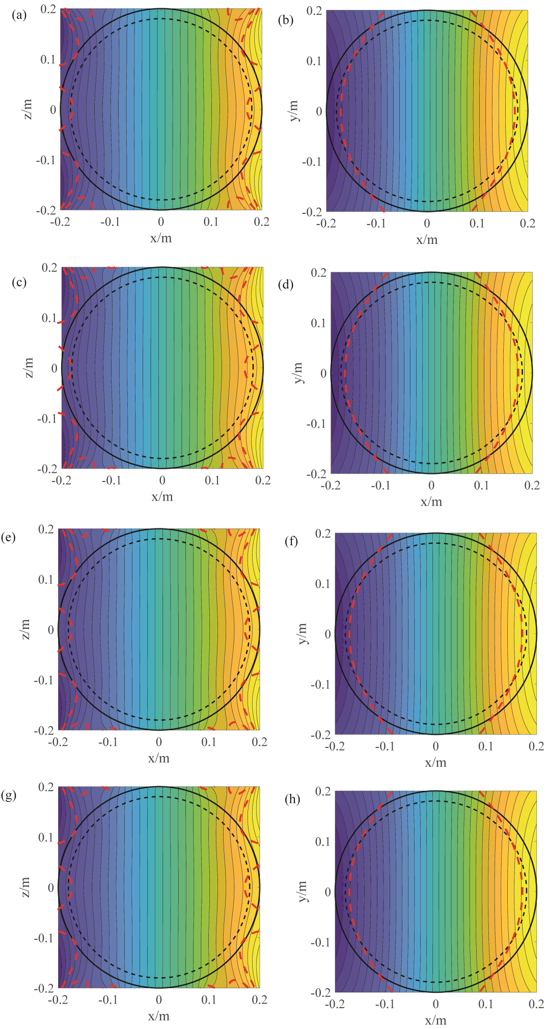
Figure 6.
A comparison of the magnetic field : (a) and (b) are the magnetic field for proposed coils (
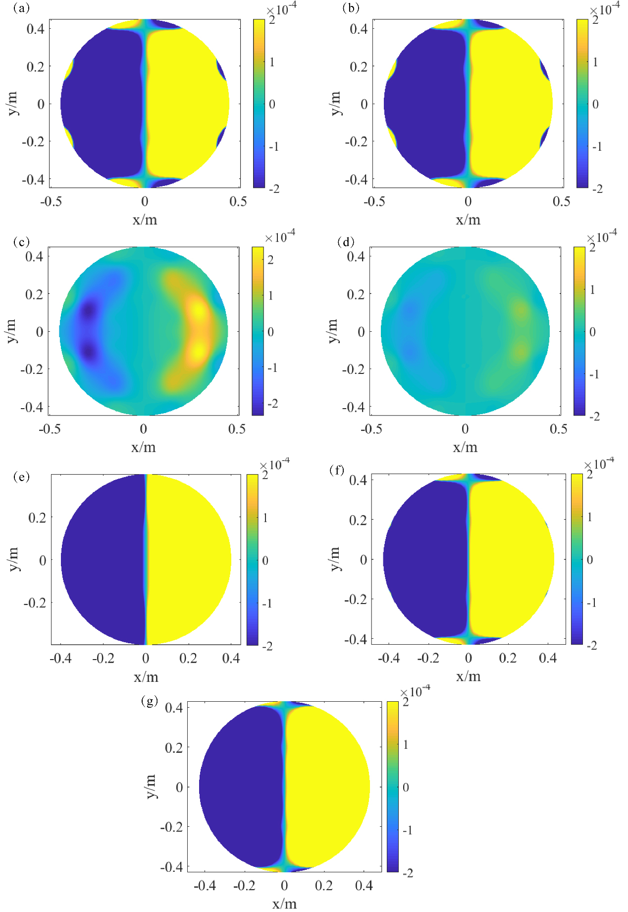
Figure 7.
A comparison of
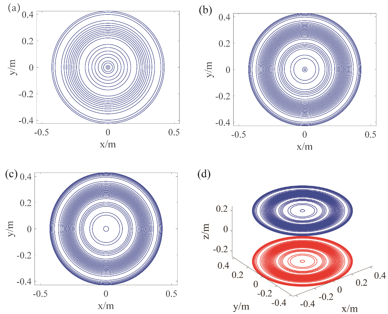
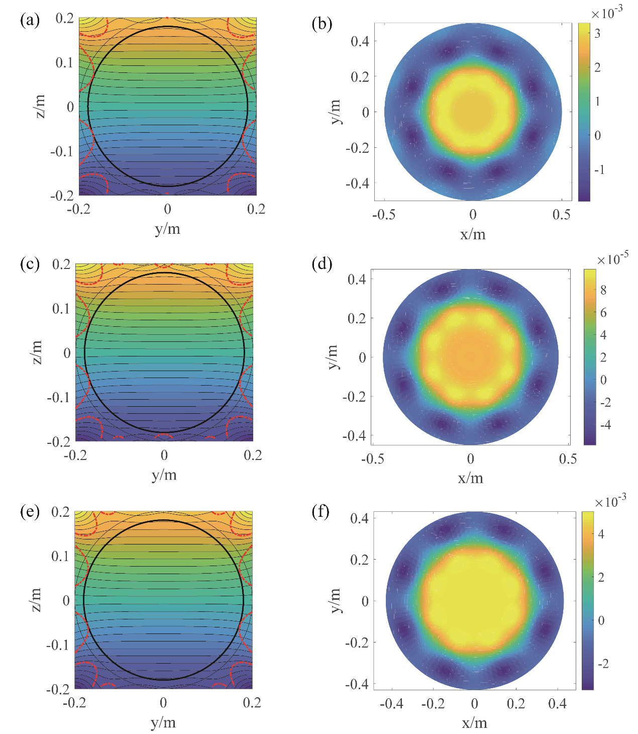
Figure 8.
Magnetic field distribution for the proposed
The magnetic field error and linearity produced by the different cases (as depicted in Table 2) are listed in Fig. 5. The magnetic field distribution of both the shielded and unshielded coils in DSV region present a similar linear variation for the x axis because the same target field and dimensions constraints (magnetic field error:
The magnetic field distributions for the shielding plate are illustrated in Fig. 6, however, the stray field distributions are quite different. For comparison, the magnetic field distributions on the sampling plane of unshielded and actively shielded coils are plotted, as depicted in Fig. 6e–g. The leaking magnetic field distributions of the coil patterns (
Figure 7 displays the proposed coils for the different cases and unshielded z-gradient coil patterns. The unshielded coil plane (radius 0.43 m) was located on
4.Conclusion
In this paper, a novel planar gradient coil design theoretical framework was proposed, which is beneficial to the development of permanent MRI device systems. The designed coil set can be used for planar MRI system by using resist-eddy current plate to eliminate the eddy currents, and combined the finite difference with mirror-image theory into the gradient coils design process, without using the actively shielded that usually requiring high currents. According to the results of the numerical calculation, for the x-gradient coil, the operating currents in the cases were reduced by 34.4% by replacing the active shielding using mirror-image theory, while a performance metric for the properties was maintained in this study. The performance of the coil will be re-verified evaluation in vivo experiments.
Acknowledgments
This study is supported by the National Natural Science Foundation of China (Grant No. 51605385), the Natural Science Foundation of Shaanxi Province (Grant No. 2017JQ5026), the Fundamental Research Funds for the Central Universities (Grant No. 3102017zy008), the Guangdong Basic and Applied Basic Research Foundation (Grant No.2019A1515111176), the Guangdong Science and Technology Innovation Strategy Special Foundation (2019B090904007), and the Shaanxi Provincial Key R&D Program (2020KW-058).
Conflict of interest
None to report.
References
[1] | Wang WD, Zhang P, Shi YK, Jiang QQ, Zou YJ. Design and Compatibility Evaluation of Magnetic Resonance Imaging-Guided Needle Insertion System. J Med Imaging Health Inform. (2015) ; 5: (8): 1963-1967. |
[2] | Wang LQ, Wang WM. Multi-objective optimization of gradient coil for benchtop magnetic resonance imaging system with high-resolution. Chin Phys B. (2014) ; 23: (2): 8. |
[3] | Zhang P, Shi YK, Wang WD, Wang YH. A spiral, bi-planar gradient coil design for open magnetic resonance imaging. Technology and Health Care. (2018) ; 26: (1): 119-132. |
[4] | Trakic A, Liu F, Lopez HS, Wang H, Crozier S. Longitudinal gradient coil optimization in the presence of transient eddy currents. Magnetic Resonance in Medicine. (2007) ; 57: (6): 1119-1130. |
[5] | Li X, Xia L, Liu F, Crozier S, Xie DX. Characterization and Reduction of X-Gradient Induced Eddy Currents in a NdFeB Magnetic Resonance Imaging Magnet-3D Finite Element Method-Based Numerical Studies. Concepts Magn. Reson. Part B. (2011) ; 39B: (1): 47-58. |
[6] | Tang FF, Freschi F, Repetto M, Li Y, Liu F, Crozier S. Mitigation of intra-coil eddy currents in split gradient coils in a hybrid MRI-LINAC system. IEEE Trans Biomed Eng. (2017) ; 64: (3): 725-732. |
[7] | Wang YH, Liu F, Zhou XR, Li Y, Crozier S. A numerical study of the acoustic radiation due to eddy current-cryostat interactions. Medical Physics. (2017) ; 44: (6): 2196-2206. |
[8] | Gilbert KM, Klassen LM, Menon RS. A low-cost, mechanically simple apparatus for measuring eddy current-induced magnetic fields in MRI. NMR Biomed. (2013) ; 26: (10): 1285-1290. |
[9] | Zhu MH, Xia L, Liu F, Crozier S. Deformation-space method for the design of biplanar transverse gradient coils in open MRI systems. IEEE Trans Magn. (2008) ; 44: (8): 2035-2041. |
[10] | Forbes LK, Crozier S. Novel target-field method for designing shielded biplanar shim and gradient coils. IEEE Trans Magn. (2004) ; 40: (1): 1929-1938. |
[11] | Zhang R, Xu J, Fu YY, et al. An optimized target-field method for MRI transverse biplanar gradient coil design. Meas Sci Technol. (2011) ; 22: (12): 7. |
[12] | Moon C, Park H, Lee S. A design method for minimum-inductance planar magnetic-resonance-imaging gradient coils considering the pole-piece effect. Meas Sci Technol. (1999) ; 10: (12): N136. |
[13] | Zu DL, Hong LM, Cao XM, Tang X. Analysis on background magnetic field to generate eddy current by pulsed gradient of permanent-magnet MRI. Sci China-Technol Sci. (2010) ; 53: (1): 886-891. |
[14] | Xu YJ, Lopez HS, Chen QY, Yang XD. Pole plate effected gradient coils design in permanent magnet MRI system. Concepts Magn. Reson. Part B. (2016) ; 46: (1): 169-177. |
[15] | Juhas A, Pekarić-Na N, Toepfer H. Magnetic field of rectangular current loop with sides parallel and perpendicular to the surface of high-permeability material. Serbian Journal of Electrical Engineering. (2014) ; 11: (1): 701-717. |
[16] | Zhu MH, Xia L, Liu F, Zhu JF, Kang LY, Crozier S. A finite difference method for the design of gradient coils in MRI-an initial framework. IEEE Trans Biomed Eng. (2012) ; 59: (9): 2412-2421. |
[17] | Zhu MH, Shou GF, Xia L, et al. A finite-difference method for the design of biplanar transverse gradient coil in MRI. 2010 4th International Conference on Bioinformatics and Biomedical Engineering. New York: IEEE; (2010) . |
[18] | Brideson MA, Forbes LK, Crozier S. Determining complicated winding patterns for shim coils using stream functions and the target-field method. Concepts in Magnetic Resonance. (2002) ; 14: (1): 9-18. |
[19] | Hu Y, Wang QL, Zhu XC, Niu CQ, Wang YH. Optimization magnetic resonance imaging shim coil using second derivative discretized stream function. Concepts Magn Reson Part B. (2017) ; 47B: (1): 10. |
[20] | Forbes LK, Brideson MA, Crozier S. A target-field method to design circular biplanar coils for asymmetric shim and gradient fields. IEEE Trans Magn. (2005) ; 41: (6): 2134-2144. |
[21] | Lemdiasov RA, Ludwig R. A stream function method for gradient coil design. Concepts Magn Reson Part B. (2005) ; 26B: (1): 67-80. |
[22] | Lopez HS, Liu F, Poole M, Crozier S. Equivalent magnetization current method applied to the design of gradient coils for magnetic resonance imaging. IEEE Trans Magn. (2009) ; 45: (2): 767-775. |
[23] | Wang YH, Wang QL, Guo L, Chen ZF, Niu CQ, Liu F. An actively shielded gradient coil design for use in planar MRI systems with limited space. Review of Scientific Instruments. (2018) ; 89: (9): 8. |
[24] | Kamon M, Tsuk MJ, White JK. Fasthenry – A multipole-accelerated 3-D inductance extraction program. IEEE Trans Microw Theory Tech. (1994) ; 42: (9): 1750-1758. |


