
Classification of fissured tongue images using deep neural networks
Abstract
BACKGROUND:
Tongue inspection is vital in traditional Chinese medicine. Fissured tongue is an important feature in tongue diagnosis, and primarily corresponds to three Chinese medicine syndromes: syndrome-related hotness, blood deficiency, and insufficiency of the spleen. Diagnosis of the syndrome is significantly affected by the experience of clinicians, and it is difficult for young doctors to perform accurate diagnoses.
OBJECTIVE:
The syndrome not only depends on the local features based on fissured regions but also on the global features of the whole tongue; therefore, a syndrome diagnosis framework combining the global and local features of a fissured tongue image was developed in the present study to achieve a quantitative and objective diagnosis.
METHODS:
First, we detected the fissured region of a tongue image using a single-shot multibox detector. Second, we extracted the global and local features from a whole tongue image and a fissured region using TongueNet (developed in-house). Third, we developed a classifier to determine the final syndrome.
RESULTS:
Based on an experiment involving 721 fissured tongue images, we discovered that TongueNet affords better feature extraction. The accuracy of TongueNet was 4% (
CONCLUSIONS:
Our findings indicate that TongueNet designed with batch normalization and dropout is more suitable for uncomplicated images than InceptionV3 and ResNet18. In addition, compared with the global features, the fusion features supplement the detailed information of the fissures and improve classification accuracy.
1.Introduction
Tongue diagnosis is vital in traditional Chinese medicine (TCM). According to TCM, the tongue is closely related to the health of the individual. Different characteristics (such as shape and color) of the tongue can reflect internal health and the severity or progression of disease. TCM practitioners evaluate clinical symptoms and select appropriate treatments by observing tongue characteristics; however, traditional tongue diagnosis is based on subjective observation and is often affected by personal experience, variation in environmental lighting, etc. [1]. Therefore, a quantitative and objective diagnostic method for issues related to the tongue must be developed.
In recent years, owing to the development of computer techniques, the application of digital image processing has been widely investigated with respect to tongue diagnosis. We cannot disregard new possibilities for improving TCM using computer technologies, such as segmentation of the tongue image [2, 3, 4], separation of tongue substances and tongue coating [5, 6], and analysis of tongue images [1, 7, 8, 9, 10, 11, 12, 13]. Ning et al. [4] presented a region merging-based automatic tongue segmentation method. In addition, using the hue, saturation, and value color space, Kamarudin et al. [5] devised new color-brightness threshold parameters to improve the efficiency of tongue substance and coating separation and shadow elimination. In the analysis of tongue images, researchers typically combine handcrafted features based on colors and shapes with the support vector machine (SVM), decision tree, and other classification models. Wang et al. [11] proposed a method that uses the information from convex defects of the tongue to recognize a tooth-marked tongue. Zhang et al. [1, 12] proposed an objective and systematic tongue color analysis system. Using the tongue color gamut, 12 standard tongue colors were quantitated. The tongue color feature vector was composed of the ratio of each color for the entire image.
In the Color Atlas of Chinese Medical Tongue Diagnosis, edited by Xu [14], a fissured tongue is defined by several shapes, such as cracks and fissures, on the surface of a tongue that differ in depth and number. The syndrome is a term in TCM, referring to the generalization of pathological attributes at a certain stage in the course of disease development. According to TCM theory, three types of syndromes correspond to a fissured tongue: syndrome-related hotness, blood deficiency, and insufficiency of the spleen. Syndrome-related hotness manifests as a reddish tongue and a rough fissured area; however, blood deficiency exhibits characteristics such as a white tongue with a fissured area. Meanwhile, insufficiency of spleen performance is reflected by fissures along with tooth-marked regions and a thick fur.
Even though fissured tongue is vital to the clinical practice of TCM, only a few studies have been conducted for digital analysis of images. Wang et al. [15] used the gray difference method to extract the fissure contour as well as calculate the fissure length, width, average gray value, and other parameters for construction of the feature vector. Zhang et al. [16] compared the performance of the watershed algorithm and the Weber local descriptor in fissure extraction, and discovered that the former performed better; however, Zhang focused only on identifying tagged pixels of fissures with certain thresholds without using an effective classifier. Therefore, Li et al. [17] improved Zhang’s method using the Otsu threshold and histogram equalization. Finally, an SVM was used to recognize fissured tongue, and the identification accuracy increased.
In general, although previous studies have realized significant achievements in the field of fissured tongue recognition, some important issues still need to be explored. Firstly, the sample size of the datasets was relatively small (e.g., less than 1000 for [15, 16, 17]), which may restrict the generalization of the classification models. Secondly, all methods used handcrafted features, although some minor details were difficult to describe. Finally, the studies focused on the method to identify fissured tongue, whereas the syndrome related to fissured tongue was not investigated.
The remainder of this paper is organized as follows: in Section 2, our dataset and the specific procedures pertaining to the proposed method are described; the experimental results are presented in Section 3; and the conclusions and discussion of future studies are provided in Section 4.
Figure 1.
Illustration of the architecture of the syndrome diagnosis model.
2.Materials and methods
Figure 1 summarizes the framework of the experimental design used in our study. We first preprocessed the collected fissured tongue data (segmentation, resizing, and labeling). A single-shot multibox detector (SSD) [18] was used to obtain the fissured region. Subsequently, the global and local features were extracted separately from the whole image, and the fissured region was detected using our proposed network, named G-TongueNet and L-TongueNet. After feature extraction, we concatenated the features in the channel dimension. Subsequently, a gradient-boosting decision tree (GBDT) [19] was used to classify the three syndromes: syndrome-related hotness, blood deficiency, and insufficiency of the spleen.
2.1Dataset
We collected 3,322 subjects from Heilongjiang University of Chinese Medicine from April 2018 to December 2019. The exclusion criteria for this study were the black race, white race, and subjects with serious mental problems, organic diseases, and cardiac pacemakers. The Institutional Review Boards reviewed the data, and approval was obtained from Heilongjiang University of Chinese Medicine. Written informed consent was obtained from each subject. The overall mean
The dataset was composed of 3322 tongue images measuring either 1480
2.2Image preprocessing
To maintain the size of the input image, the original pre-segmented tongue image must be scaled. We used the OpenCV toolbox to achieve long-term proportional scaling to 300
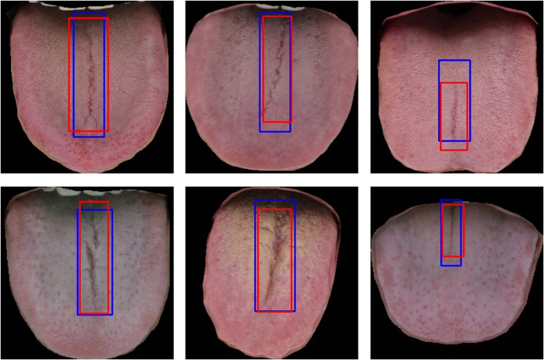
In this study, we labeled the fissured region using BBox-Label-Tool (https://github.com/NorrisWu/BBox-Label-Tool-master). After identifying the location, the boundary box was saved as (x, y, w, l), where x and y represent the top-left coordinates, and w and l denote the width and height, respectively. Finally, a four-element integer vector was saved to the notepad. Figure 2 shows three samples of tongue images with labels.
Figure 2.
Examples of labeled fissured regions.
2.3Fissured region detection
To learn the features of the fissured region in the tongue image, the region must first be detected. However, the color contrast between the fissured region and its surrounding tissue was unclear, and traditional target detection methods based on hand-designed features often cannot satisfy the requirements. Therefore, at this stage, we used a convolutional neural network (CNN) to determine the fissured region.
We used an SSD in this study, the architecture of which is shown in Fig. 3. The SSD uses a visual geometry group network (VGG16, including 13 convolutional layers and 3 fully connected layers) [20] as the backbone network. The last two fully connected layers were changed to convolutional layers, after which four convolutional layers were added. For an input image, the model first extracts feature maps of different sizes from the backbone network. After another convolutional layer and a pooling layer, every pixel in these feature maps will generate several default boxes of different sizes. Consequently, fissures of different scales can be detected. For every default box, we predicted the category, calculated the classification loss and position loss using the gold standard, and performed training to minimize the loss. Finally, non-maximum suppression was performed to filter overlapping boundary boxes.
Figure 3.
Fissured region detection network structure.
A total of 2601 fissured tongue images were assigned to a training set (70%) or a test set (30%). The training set included 1820 fissured tongue images, and the test set included 781 fissured tongue images. We used stochastic gradient descent to adjust our network to a batch size of 50, a learning rate of 0.0001, a weight decay of 0.0005, and an iteration of 50,000. The non-maximum suppression method was used to filter a part of the overlapping boundary boxes, and we set the overlap rate threshold to 0.6.
During testing, every image was calculated with the fixed weight from the SSD, and the fissured region was output.
2.4Feature extraction
We designed a CNN model named TongueNet to extract both global and local fissured tongue features. These features were used to classify the three syndromes: syndrome-related hotness, blood deficiency, and insufficiency of the spleen.
TongueNet is improved from LeNet [21], which solves the shortcomings of LeNet, i.e., it overfits easily by adding a batch normalization [22] layer and dropout [23]. Furthermore, to ensure that TongueNet learns the features of the fissured tongue image while reducing the training time and parameter calculation, the number of layers was not fixed, and the best model depth was obtained through experimental design.
Figure 4.
Fissure feature extraction model based on G-TongueNet.
The TongueNet architecture used in this study is shown in Fig. 4. TongueNet is primarily composed of several blocks that contain one convolutional layer, one BN layer, and one pooling layer. TongueNet adjusts the depth by increasing or decreasing the number of blocks. Considering the size of the input image, a larger kernel (5
TongueNet that extracts local and global features of fissured tongue images is named L-TongueNet and G-TongueNet, respectively. The grid search method was used to determine the best parameters of TongueNet. L-TongueNet achieved the best performance with a learning rate of 0.0001, a weight decay of 0.1, a drop rate of 0.2, a batch size of 60, and a block number of 8. We stopped our training after 500 epochs. Furthermore, G-TongueNet was used to determine the parameters using the grid search method. The main difference between L-TongueNet and G-TongueNet is that the former has 8 blocks, but the latter has 7 blocks. In addition, InceptionV3 [25, 26] and ResNet18 [27] were trained for comparison.
During testing, the network served as a fixed feature extractor. We eliminated the last layer of Softmax and output the pre-layer as deep features; therefore, we extracted global features from the original fissured tongue image and local features from the fissured region detected by the SSD. All these features were used to classify the three syndromes. Although the network can output the classification directly, we discovered that the fusion features were better. Comparisons and analyses are shown in Section 3.
2.5Classification of syndromes
At this stage, the global and local features were concatenated in the channel dimension. Subsequently, the GBDT was trained to classify the three syndromes. The GBDT builds multiple decision trees sequentially, where each decision tree is built on the residual from the previous decision tree.
Two classic classifiers, the SVM and back propagation (BP) neural networks [28, 29], were used for model comparison. The experimental results were evaluated using the following six metrics: (1) accuracy; (2) sensitivity; (3) specificity; (4) time complexity; (5) space complexity; and (6) number of parameters [30].
To eliminate the effects of accidental factors on the accuracy of the model, bootstrap and permutation tests were performed. All confidence intervals were computed based on the percentiles of 1,000 random resamplings (bootstraps) of the data. The accuracy difference and p-values were calculated by a standard permutation test [31] using 10,000 random resamplings of the test set. Firstly, the test set was sampled repeatedly to obtain two sample groups, which were respectively input to model A and model B. Subsequently, the accuracy difference between model A and model B was calculated; repeating 10,000 times, obtains 10,000 differences. Finally, we obtained the average accuracy difference. The confidence interval and p-value were also calculated from the 10,000 differences.
3.Results and discussion
3.1Results of fissured region detection
A total of 733 fissured regions were correctly detected, and the precision, recall, and mAP reached 0.81, 0.88, and 0.85, respectively. Figure 5 shows some fissured regions detected by the SSD in the test set. The results indicate that: 1) the SSD performance was good, i.e., 88% of fissures with all shapes were detected; and 2) some small fissures were overlooked. This was because small fissures, typically with shallow depths, have a similar contrast to surrounding tissue and hence are difficult to detect.
Figure 5.
Some fissured regions detected by SSD.
3.2Global and local features
We conducted the experiments on our dataset using two additional illustrious methods, i.e., ResNet18 and InceptionV3. Using the training strategy described in feature extraction, we trained L-ResNet18 and L-InceptionV3 from the fissured regions and G-ResNet18 and G-InceptionV3 from the whole tongue images.
Table 1
Comparison of the classification metrics of different global feature learning models
| Model | Accuracy | Sensitivity | Specificity | AUC | |
|---|---|---|---|---|---|
| Syndrome-related hotness | G-TongueNet | 0.86 | 0.88 | 0.83 | 0.81 |
| G-ResNet18 | 0.85 | 0.90 | 0.76 | 0.75 | |
| G-InceptionV3 | 0.79 | 0.81 | 0.74 | 0.77 | |
| Blood deficiency | G-TongueNet | 0.79 | 0.82 | 0.75 | 0.75 |
| G-ResNet18 | 0.79 | 0.82 | 0.74 | 0.83 | |
| G-InceptionV3 | 0.81 | 0.88 | 0.68 | 0.78 | |
| Insufficiency of the spleen | G-TongueNet | 0.83 | 0.92 | 0.65 | 0.82 |
| G-ResNet18 | 0.80 | 0.86 | 0.67 | 0.84 | |
| G-InceptionV3 | 0.84 | 0.88 | 0.71 | 0.82 |
Figure 6.
ROC of the global feature models.
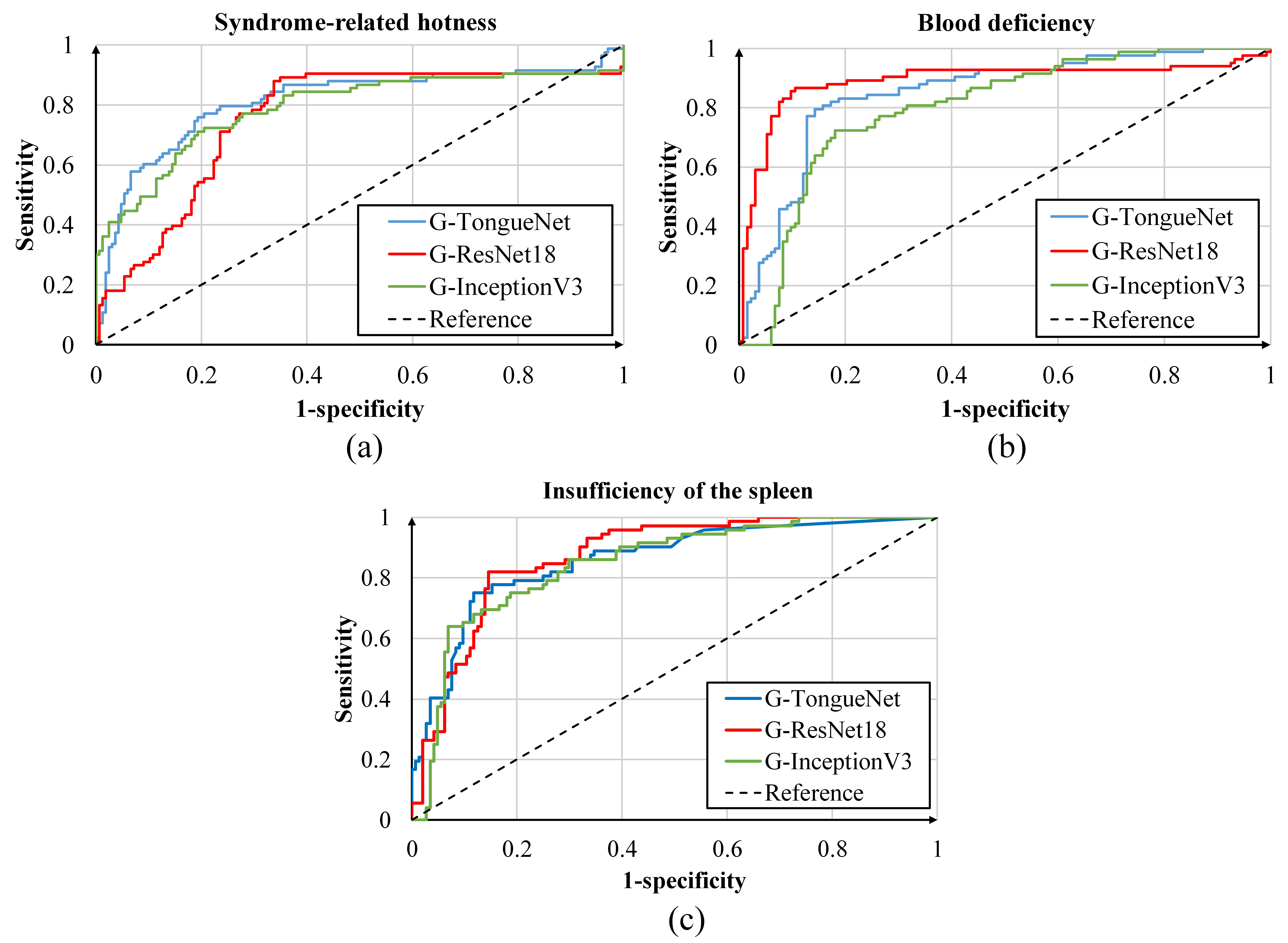
To illustrate the results more clearly, we constructed a receiver operating characteristics (ROC) curve of each syndrome, as shown in Fig. 6. Furthermore, we calculated the accuracy, sensitivity, specificity, and area under the curve (AUC) values, as shown in Table 1. Although G-TongueNet indicated the highest AUC value in the classification of syndrome-related hotness, ResNet18 attained the maximum AUC value in the classification of blood deficiency and insufficiency of the spleen. Different models attained their maximum values under different syndromes and metrics.
Table 2
Comparison of the complexity and overall accuracy of different global feature learning models
| Number of parameters (MB) | Time complexity (GFLOPs) | Space complexity (MB) | Overall accuracy (95% CI) | Accuracy difference (95% CI) | |
|---|---|---|---|---|---|
| G-ResNet18 | 42.66 | 9.58 | 54.63 | 0.72 | |
| (0.691, 0.742) | ( | ||||
| G-TongueNet | 1.04 | 1.19 | 30.30 | 0.75 | |
| (0.704, 0.798) | |||||
| G-InceptionV3 | 453.00 | 9.80 | 510.80 | 0.71 | ( |
| (0.664, 0.728) |
Figure 7.
ROC of local feature models.
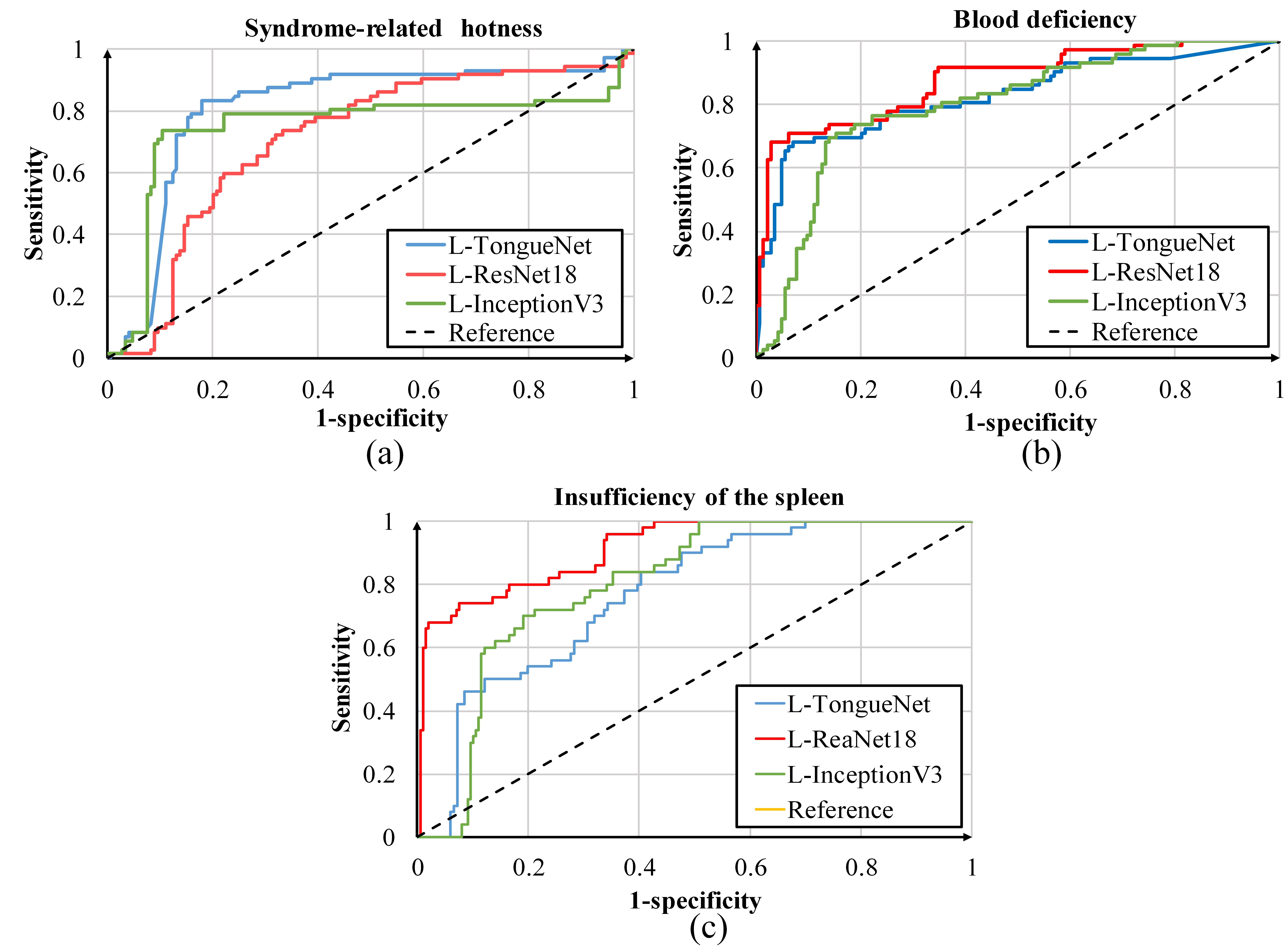
Table 2 shows the metrics of different global feature learning models. To avoid the contingency of the test set, we used bootstrap to resample the test set 1000 times and calculated the 95% confidence interval. The accuracy difference, representing the average difference in accuracy between two models in 10,000 permutation tests, and the p-value were also calculated. Firstly, the accuracy difference was valid and a p-value less than 0.005 signifies that G-TongueNet was better than G-ResNet18 and G-InceptionV3. Meanwhile, G-TongueNet performed better in terms of the number of parameters, time complexity, and space complexity. It can be concluded that G-TongueNet can significantly reduce the training time and model storage cost while obtaining the best deep features.
Table 3
Comparison of the classification metrics between different local feature learning models
| Model | Accuracy | Sensitivity | Specificity | AUC | |
|---|---|---|---|---|---|
| Syndrome-related hotness | L-TongueNet | 0.82 | 0.82 | 0.81 | 0.80 |
| L-ResNet18 | 0.80 | 0.81 | 0.76 | 0.78 | |
| L-InceptionV3 | 0.77 | 0.82 | 0.69 | 0.77 | |
| Blood deficiency | L-TongueNet | 0.85 | 0.86 | 0.83 | 0.80 |
| L-ResNet18 | 0.85 | 0.84 | 0.87 | 0.82 | |
| L-InceptionV3 | 0.82 | 0.86 | 0.75 | 0.79 | |
| Insufficiency of the spleen | L-TongueNet | 0.72 | 0.90 | 0.52 | 0.76 |
| L-ResNet18 | 0.73 | 0.93 | 0.54 | 0.83 | |
| L-InceptionV3 | 0.75 | 0.85 | 0.64 | 0.79 |
Similar to the global feature extraction experiment, we constructed the ROC curve and created a metric table from the local feature extraction experiment, as shown in Fig. 7 and Table 3. The results show that L-TongueNet, L-ResNet18, and L-InceptionV3 yielded similar performance, and no particular method triumphed in all metrics.
Table 4
Comparison of the complexity and overall accuracy of different local feature learning models
| Number of parameters (MB) | Time complexity (GFLOPs) | Space complexity (MB) | Overall accuracy (95% CI) | Accuracy difference (95% CI) | |
|---|---|---|---|---|---|
| L-ResNet18 | 42.66 | 9.58 | 54.63 | 0.72 | |
| (0.679, 0.735) | ( | ||||
| L-TongueNet | 1.09 | 1.19 | 30.30 | 0.72 | |
| (0.682, 0.748) | |||||
| L-InceptionV3 | 453.00 | 9.80 | 510.80 | 0.69 | ( |
| (0.655, 0.724) |
Furthermore, the number of parameters, space complexity, time complexity, and overall accuracy are shown in Table 4. Similarly, L-TongueNet performed the best in terms of number of parameters, space complexity, and time complexity. Although L-TongueNet performed better than L-InceptionV3, it exhibited the same overall accuracy as L-ResNet18. The results indicate that L-TongueNet and L-ResNet18 possessed the same feature extraction capabilities, which were better than those of L-InceptionV3. Additionally, L-InceptionV3 trained 415 times more parameters than L-TongueNet and exhibited worse accuracy due to overfitting.
3.3Classification results
From the experiments in the last part, it is evident that G-TongueNet and L-TongueNet performed the best in terms of global and local feature extraction; therefore, we used the 128-dimensional deep feature at the last fully connected layer of the G-TongueNet and L-TongueNet as the output. In this experiment, 721 tongue images were segmented into a training set and a test set at a ratio of 7:3. The training and test sets contained 505 and 216 images, respectively. Based on the model structure described in Section 2, after the fusion of global and local features, we used the GBDT to classify the syndromes. In addition, the SVM and BP networks were used for comparison.
Using the grid search method to adjust the parameters, we discovered that the linear kernel SVM with cost C
Table 5
Comparison of the classification metrics of different classifiers
| Model | Accuracy | Sensitivity | Specificity | AUC | |
|---|---|---|---|---|---|
| Syndrome-related hotness | SVM | 0.88 | 0.90 | 0.82 | 0.88 |
| GBDT | 0.88 | 0.88 | 0.86 | 0.88 | |
| BP | 0.86 | 0.88 | 0.81 | 0.85 | |
| Blood deficiency | SVM | 0.82 | 0.85 | 0.78 | 0.84 |
| GBDT | 0.85 | 0.88 | 0.75 | 0.81 | |
| BP | 0.85 | 0.88 | 0.81 | 0.86 | |
| Insufficiency of the spleen | SVM | 0.83 | 0.90 | 0.72 | 0.78 |
| GBDT | 0.82 | 0.90 | 0.70 | 0.73 | |
| BP | 0.81 | 0.90 | 0.70 | 0.75 |
Figure 8.
ROC of different classifiers.
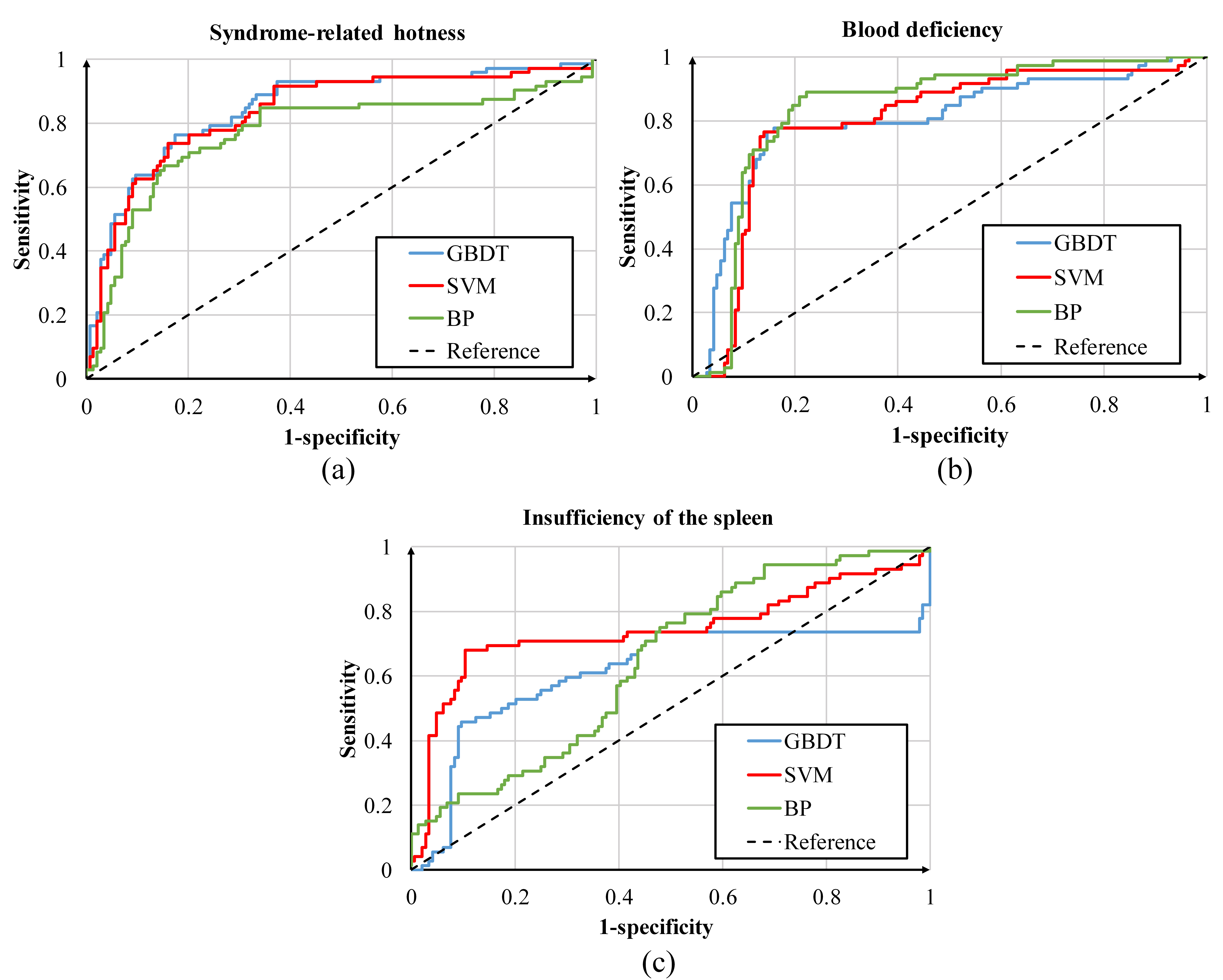
Figure 8 shows the ROC curve of each syndrome, and Table 5 shows the accuracy, sensitivity, specificity, and AUC. In terms of syndrome-related hotness and blood deficiency, the three curves were relatively close to each other; however, in terms of insufficiency of the spleen, the three curves differed, wherein the SVM performed better. Meanwhile, Table 5 shows the performance of the three methods more clearly. We discovered that in syndrome-related hotness classification, the GDBT achieved the highest accuracy, specificity, and AUC values; however, the SVM achieved the best accuracy, sensitivity, and AUC values. In blood deficiency classification, the GBDT achieved the highest accuracy and sensitivity values, but the BP network achieved the highest values for all metrics. Finally, in terms of insufficiency of the spleen, the SVM achieved the highest accuracy, specificity, and AUC values, whereas the three methods exhibited the same sensitivity value. It is noteworthy that, for some metrics, different classifiers achieved the highest value simultaneously; therefore, we believe that the difference among the three classifiers was minimal.
Table 6
Comparison of overall accuracy and accuracy difference of different classifiers
| Model | Overall accuracy (95% CI) | Accuracy difference (95% CI) |
|---|---|---|
| SVM | 0.77 | |
| (0.754, 0.789) | ( | |
| GBDT | 0.78 | |
| (0.747, 0.801) | ||
| BP | 0.77 | ( |
| (0.733, 0.796) |
Furthermore, we calculated the overall accuracy of the three classifiers, as shown in Table 6. The GBDT exhibited minimal advantages; however, from the results of the permutation test, we discovered no significant difference in the model accuracy (
Table 7
Comparison of the overall accuracy and difference in the accuracy of models based on different features
| Model | Overall accuracy (95% CI) | Accuracy difference (95% CI) |
|---|---|---|
| Model based on global features | 0.75 | |
| (0.704, 0.789) | ( | |
| Model based on fusion features | 0.78 | |
| (0.747, 0.801) | ||
| Model based on local features | 0.72 | ( |
| (0.682, 0.748) |
In addition, the classification results of G-TongueNet and L-TongueNet were compared with those of the fusion feature model using the GDBT. The results are shown in Table 7. The accuracy of the model using fusion features was 3% higher than that of G-TongueNet and 5% higher than that of L-TongueNet. After 1000 bootstrap replications, the average accuracy difference was calculated. Moreover, our fusion feature model still surpassed G-TongueNet and L-TongueNet by 2.5% and 5.3%, respectively. We believe that our method, which combines global and local features, can improve the accuracy of classification in syndromes.
4.Conclusion
Herein, we propose a framework for the classification of fissured tongue images using deep neural networks. Firstly, we completed the automatic detection of a fissured region from a tongue using an SSD. The experimental results indicate that TongueNet performed better than InceptionV3 and ResNet18 in feature extraction. Moreover, TongueNet performed better in time complexity and space complexity. The results suggest that a shallow network can extract better features from uncomplicated fissured tongue images. Finally, it was discovered that the fusion features possessed higher accuracy than the global or local features. This validated that the fusion features supplemented the detailed information of the fissures and yielded better performance. Using the framework, we achieved a quantitative and objective diagnosis of syndromes. Further, our method requires less storage space and less time. In future studies, we will investigate the fusion of other forms of information including pulse waves and facial information to improve the accuracy of diagnosis.
Acknowledgments
This work was supported by the National Key Research and Development Program of China (Grant no. 2018YFC1707704).
Conflict of interest
None to report.
References
[1] | Zhang B, Wang XZ, You J, Zhang D. Tongue color analysis for medical application. Evidence-Based Complementray and Alternative Medicine. (2013) ; 2013: : 264-742. doi: 10.1155/2013/264742. |
[2] | Kamarudin ND, Ooi CY, Kawanabe T, et al. A fast and effective segmentation algorithm with automatic removal of ineffective features on tongue images. Jurnal Teknologi. (2016) ; 78: (8): 153-163. doi: 10.11113/jt.v78.7129. |
[3] | Zhu MF, Du JQ. A novel approach for color tongue image extraction based on random walk algorithm. Applied Mechanics & Materials. (2013) ; 462-463: : 338-342. doi. 10.4028/www.scientific.net/AMM.462-463.338. |
[4] | Ning J, Zhang D, Wu C, Feng Y. Automatic tongue image segmentation based on gradient vector flow and region merging. Neural Computing & Applications, (2012) ; 21: (8): 1819-1826. doi: 10.1007/s00521-010-0484-3. |
[5] | Kamarudin ND, Ooi CY, Kawanabe T, et al. Tongue’s substance and coating recognition analysis using HSV color threshold in tongue diagnosis. First International Workshop on Pattern Recognition. (2016) ; 100110. doi: 10.1117/12.2242404. |
[6] | Kim KH, Do JH, Ryu H, Kim JY. Tongue diagnosis method for extraction of effective region and classification of tongue coating. First Workshops on Image Processing Theory, Tools and Applications. (2008) ; 1-7. doi: 10.1109/IPTA.2008.4743772. |
[7] | Wang X, Liu JW, Wu CY, Liu JH, et al. Artificial intelligence in tongue diagnosis: Using deep convolutional neural network for recognizing unhealthy tongue with tooth-mark. Computational & Structural Biotechnology Journal. (2020) ; 18: : 973-980. doi: 10.1016/j.csbj.2020.04.002. |
[8] | Li XQ, Zhang Y, et al. Tooth-marked tongue recognition using multiple instance learning and cnn features. IEEE Transactions on Cybernetics. (2019) ; 49: (2), 380-387. doi: 10.1109/TCYB.2017.2772289. |
[9] | Cao GT, Ding J, Duan Y, Tu LP, Xu JT, Xu D. Classification of tongue images based on doublet and color space dictionary. 2016 IEEE International Conference on Bioinformatics and Biomedicine. (2016) ; 1170-1175. doi: 10.1109/BIBM.2016.7822686. |
[10] | Qi Z, Tu LP, Chen JB, et al. The classification of tongue colors with standardized acquisition and icc profile correction in traditional chinese medicine. BioMed Research International. (2016) ; 2016: : 1-9. doi: 10.1155/2016/3510807. |
[11] | Wang H, Zhang XF, Cai YH. Research on teeth marks recognition in tongue image. in 2014 International Conference on Medical Biometrics, IEEE: 2014. pp. 80-84. doi: 10.1109/ICMB.2014.21. |
[12] | Wang XZ, Zhang B, Yang ZM, Wang HQ, Zhang D. Statistical analysis of tongue images for feature extraction and diagnostics. IEEE Transactions on Image Processing A Publication of the IEEE Signal Processing Society. 22: (12), 5336-5347. doi: 10.1109/TIP.2013.2284070. |
[13] | Obafemi-Ajayi T, Kanawong R, Xu D, Li S, Duan Y. Features for automated tongue image shape classification. IEEE International Conference on Bioinformatics & Biomedicine Workshops: (2013) . doi: 10.1109/BIBMW.2012.6470316. |
[14] | Xu JT, Color Atlas of Chinese Medical Tongue Diagnosis. Shanghai University of TCM Press, (2009) . |
[15] | Wang HY, Zong XJ. A new computerized method for tongue classification. International Conference on Intelligent Systems Design & Applications. (2006) ; 2: : 508-511. doi: 10.1109/ISDA.2006.253889. |
[16] | Zhang HK, Hu YY, Li X, et al. Computer identification and quantification of fissured tongue diagnosis. 2018 IEEE International Conference on Bioinformatics and Biomedicine (BIBM): (2018) . doi: 10.1109/BIBM.2018.8621114. |
[17] | Li XQ, Wang D, Cui Q. WLDF: effective statistical shape feature for cracked tongue recognition. Journal of Electrical Engineering & Technology. (2017) ; 12: (1): 420-427. doi: 10.5370/JEET.2017.12.1.420. |
[18] | Liu W, Anguelov D, Erhan D, et al. SSD: Single Shot MultiBox Detector. European Conference on Computer Vision. (2016) . doi: 10.1007/978-3-319-46448-0_2. |
[19] | Lu HY, Wang HF, Yoon SW. A Dynamic Gradient Boosting Machine Using Genetic Optimizer for Practical Breast Cancer Prognosis. Expert Systems with Applications. 116: . pp. S0957417418305542. doi: 10.1016/j.eswa.2018.08.040. |
[20] | Simonyan K, Zisserman A. Very deep convolutional networks for large-scale image recognition. arXiv preprint arXiv14091556. |
[21] | Lecun Y, Bottou L, Bengio Y, Haffner P. Gradient-based learning applied to document recognition. Proceedings of the IEEE, 86: (11): 2278-2324. doi: 10.1109/5.726791. |
[22] | Ioffe S, Szegedy C. Batch normalization: Accelerating deep network training by reducing internal covariate shift. arXiv preprint arXiv150203167. |
[23] | Krizhevsky A, Sutskever I, Hinton G. ImageNet classification with deep convolutional neural networks. Advances in Neural Information Processing Systems. (2012) ; 25: (2): 1097-1105. doi: 10.1145/3065386. |
[24] | Nair V, Hinton G. Rectified linear units improve restricted boltzmann machines. in ICML: 2010. |
[25] | Szegedy C, Vanhoucke V, Ioffe S, et al. Rethinking the inception architecture for computer vision. Proceedings of the IEEE conference on computer vision and pattern recognition. (2016) ; pp. 2818-2826. doi: 10.1109/CVPR.2016.308. |
[26] | Szegedy C, Ioffe S, Vanhoucke V, Alemi A. Inception-v4, inception-resnet and the impact of residual connections on learning. Proceedings of the AAAI Conference on Artificial Intelligence: 2017. arXiv:1602.07261. |
[27] | He KM, Zhang XY, Ren SQ, Sun J. Deep residual learning for image recognition. Proceedings of the IEEE conference on computer vision and pattern recognition. (2016) ; pp. 770-778: doi: 10.1109/CVPR.2016.90. |
[28] | Zhang XY, Yang G, Bo X, et al. Application of the rough set theory and BP neural network model in disease diagnosis. 2010 Sixth International Conference on Natural Computation, pp. 167-171: IEEE: 2010. doi: 10.1109/ICNC.2010.5583303. |
[29] | Liu DL, Ling M, Hui C, Ke M. Tumor disease diagnosis model based on bp neural network. 2017 International Conference on Smart Grid and Electrical Automation (ICSGEA), pp. 308-311: IEEE: 2017. doi: 10.1109/ICSGEA.2017.72. |
[30] | Ma SJ, Cai W, Liu WK, et al. A lighted deep convolutional neural network based fault diagnosis of rotating machinery. Sensors, 19: (10), p. 2381. doi: 10.3390/s19102381. |
[31] | Chihara L, Hesterberg T. Mathematical statistics with resampling and R. Wiley Online Library, (2011) . |


