
Suppression of acoustic reflection artifact in endoscopic photoacoustic tomographic images based on approximation of ideal signals
Abstract
BACKGROUND:
In endoscopic photoacoustic tomography (EPAT), the photoacoustically induced ultrasonic wave reflects at tissue boundaries due to the acoustic inhomogeneity of the imaged tissue, resulting in reflection artifacts (RAs) in the reconstructed images.
OBJECTIVE:
To suppress RAs in EPAT image reconstruction for improving the image quality.
METHODS:
A method was presented to render the cross-sectional images of the optical absorption with reduced RAs from acoustic measurements. The ideal photoacoustic signal was recovered from acoustic signals collected by the detector through solving a least square problem. Then, high-quality images of the optical absorption distribution were reconstructed from the ideal signal.
RESULTS:
The results demonstrated the improvement in the quality of the images rendered by this method in comparison with the conventional back-projection (BP) reconstructions. Compared with the short lag spatial coherence (SLSC) method, the peak signal-to-noise ratio (PSNR), normalized mean square absolute distance (NMSAD), and structural similarity (SSIM) were improved by up to 8%, 20%, and 5%, respectively.
CONCLUSIONS:
This method was capable of rendering images displaying the complex tissue types with reduced RAs and lower computational burden in comparison with previously developed methods.
1.Introduction
Photoacoustic tomography (PAT) is a rapidly developing functional imaging modality in recent years. It provides good optical contrast and ultrasonic resolution as well as high imaging depth compared with pure optical imaging technologies [1]. Endoscopic PAT (EPAT) combines noninvasive PAT with endoscopic detection, which has a great potential in the early diagnosis of diseased tissues in a tubular object such as digestive tract and coronary vessels.
In practical applications, it is usually difficult to achieve the theoretical imaging depth because of acoustic reflection. When the PA wave propagates in different tissue types in all directions, partial wave far away from the detector may be reflected by the acoustically dense deep tissue and then propagates back to the detector which is similar to a virtual acoustic source, resulting in reflection artifacts (RAs) in the reconstructed images [2]. The RAs usually appear at a deeper depth than actual optical absorbing structures and they are easily confused with the optical absorbers to be imaged [3]. Further, RAs at a certain depth are stronger than weak PA signals generated by deep tissues, leading to the reduced imaging depth [4]. In addition, the strongly reflected clutter arising from the acoustic sources outside the imaging plane is another contributing factor leading to the limited imaging depth [5].
Early researches on RA reduction focused on clutter decorrelation. For example, Jaeger et al. [5] designed a deformation compensated averaging (DCA) approach basing on tissue palpation with the imaging probe. It requires special training for operators to control the probe motion. Moreover, it can only be employed in the epi-mode of PA imaging for easily deformable tissues such as forearm and neck, but unsuitable for EPAT. To overcome the shortcomings of DCA, Jaeger et al. [6] developed a single-focus localized vibration tagging (LOVIT) method without the need for tissue palpation. The localized tissue displacement was induced by the acoustic radiation force (ARF) generated by a focused ultrasonic beam at its focus. Different from DCA, LOVIT does not require considerable practice and training for operators. It can only be employed in the imaging system equipped with an detector which can transmit ARF beam satisfying the ultrasonic safety rules. Moreover, it takes a long time to scan the entire imaging plane since it eliminates the clutter at one focal region at a time. Later, to shorten the signal acquisition time, Petrosyan et al. [7] improved the single-focus LOVIT by creating multiple foci in parallel forming the comb-shaped ARF patterns.
The clutter decorrelation requires additional devices to acquire pulse-echo images recording tissue deformation, which prolongs the process of data acquisition. Alles et al. [8] distinguished reflected clutters and PA signals based on the difference in their spatial coherence expressed by the short-lag spatial coherence (SLSC). Compared with clutter decorrelation, SLSC needs only a single scan, which shortens the acquisition process. However, it has difficulties in distinguishing the clutter from the incoherent signal produced by dense microvascular tissues whose spatial coherence is similar to or lower than that of the clutter. Moreover, SLSC relies on time measurement of the geometric path associated with beamforming, so the reduced accuracy is observed in the case of hyperechoic reflection or strong reflection.
Recently, deep learning with convolutional neural networks (CNNs) has been widely used in medical image processing and analysis. CNN has shown its potential in recognition and removal of RAs in PA imaging [9]. The main concern is that public data sets for PAT has not been available, and the clinical case data are seriously insufficient. The data sets used in current studies are usually constructed by computer simulation. The validity of CNNs trained by such simulation data may not be guaranteed in in vivo imaging of human tissues.
This paper presents a simple method to suppress in-plane RAs in EPAT. The method recovers the approximation of ideal PA signals from acoustic measurements and numerically generated planar ultrasound. It does not require additional devices to record tissue deformation, and it is computationally efficient in comparison with CNN which requires a large amount of image data for training.
2.Method
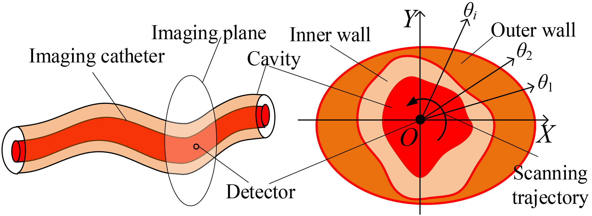
As shown in Fig. 1, an imaging catheter is inserted into the object cavity. The detector at the catheter tip circumferentially scans surrounding tissues and collects time-dependent series of acoustic pressure photoacoustically generated by optical absorbing structures. The imaging plane is perpendicular to the catheter, and the detector is located in the image center. A XOY rectangular coordinate system and a
Figure 1.
Schematic diagram of acquiring PA signal from inside a tubular object. Left: axial view. Right: transverse view.
The probe emits short laser pulses (
The photoacoustic pressure propagating in acoustically heterogeneous lossy medium satisfies the following wave equation considering both absorption and dispersion [11],
(1)
where
(2)
where
Assume that the PA wave is reflected only once during propagation. Based on the Born approximation, the pressure reaching the detector is determined by [13, 14]
(3)
where
(4)
(5)
and
(6)
Here,
The planar ultrasonic wave is numerically generated as follow,
(7)
where
(8)
and
(9)
Here,
(10)
where
The matrix form of Eq. (10) in frequency domain is
(11)
where
(12)
Here,
(13)
(14)
where
The measured acoustic signal is the superposition of the ideal signal and reflected clutter,
(15)
where
(16)
where
(17)
and
(18)
where
(19)
where I is the identity matrix.
The AOED is finally recovered from the ideal signal by back projection (BP) [15] as follow,
(20)
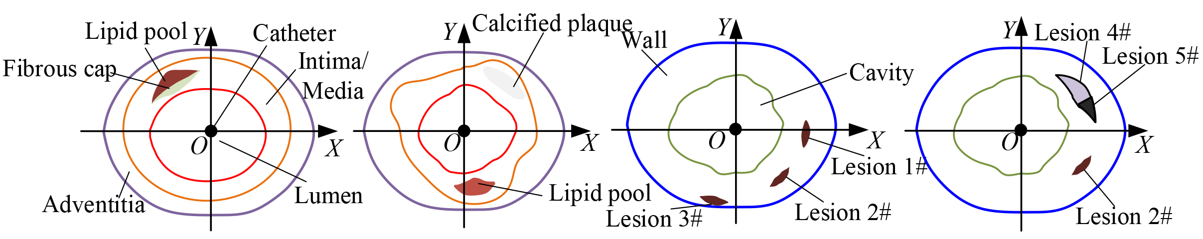
Figure 2.
Geometry of computer-simulated phantoms. From left to right, the phantoms are numbered as I, II, III, and IV.
where
3.Results
Figure 2 shows the cross-sectional geometry of the computer-simulated coronary vessel and cavity phantoms. Table 1 lists their parameters by referring to [16]. The SoS and density of each tissue layer are set as the Gauss distribution with the mean of the values in the table and the variance of 5 and 0.05, respectively.
Table 1
Optical, acoustic, and structural parameters of different tissue types in forward simulation
| Tissue name | Tissue component | Average refractive index | Average reflectivity | OAC (cm | OSC (cm | Anisotropy factor | Average SoS (m/s) | Average density (kg/L) | Average radial thickness (mm) |
|---|---|---|---|---|---|---|---|---|---|
| Vessel wall adventitia | Connective tissue | 1.42 | 0.08 | 0.21 | 6 | 0.85 | 1600 | 1.026 | Phantom I: 0.5 |
| Phantom II: 0.6 | |||||||||
| Vessel wall intima/media | Muscular tissue | 1.42 | 0.05 | 0.21 | 6 | 0.85 | 1580 | 1.073 | Phantom I: 1.0 |
| Phantom II: 1.2 | |||||||||
| Fibrous cap | Fibrous tissue | 1.47 | 0.24 | 0.018 | 25 | 0.78 | 1610 | 1.058 | 0.3 |
| Calcified plaque | Calcium | 1.47 | 0.34 | 0.62 | 560 | 0.78 | 1540 | 1.668 | 0.5 |
| Lipid pool | Lipid | 1.47 | 0.42 | 0.18 | 520 | 0.82 | 1650 | 0.947 | Phantom I: 0.3 |
| Phantom II: 0.5 | |||||||||
| lumen | Blood | 1.35 | 0.12 | 0.75 | 610 | 0.999 | 1560 | 1.065 | Phantom I: 2.0 |
| Phantom II: 1.7 | |||||||||
| Cavity wall | Connective/muscular tissue | 1.43 | 0.1 | 0.21 | 16 | 0.8 | 1600 | 1.136 | 6 |
| Lesion 1# | Effusion | 1.47 | 0.48 | 0.12 | 320 | 0.85 | 1620 | 1.087 | 1.08 |
| Lesion 2# | Tumour | 1.48 | 0.44 | 0.025 | 55 | 0.85 | 1630 | 1.112 | 1.05 |
| Lesion 3# | Fatty tissue | 1.47 | 0.45 | 0.11 | 510 | 0.85 | 1480 | 0.947 | 1.1 |
| Lesion 4# | Fibrous tissue | 1.47 | 0.24 | 0.013 | 25 | 0.85 | 1560 | 0.945 | 1.12 |
| Lesion 5# | Fibro-fatty tissue | 1.47 | 0.46 | 0.023 | 35 | 0.85 | 1580 | 1.16 | 2.5 |
| Cavity | Digestive juice | 1.2 | 0.32 | 0.52 | 620 | 0.999 | 1540 | 1.005 | 5 |
Figure 3.
Images of AOED (top) and initial pressure (bottom) by forward simulation.
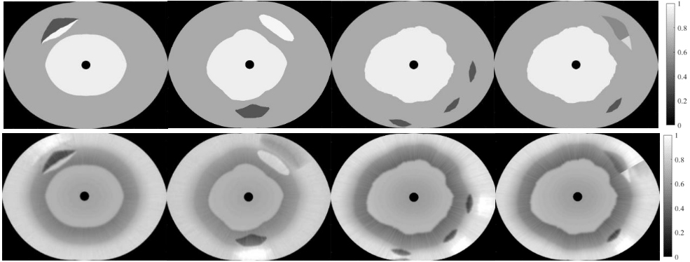
Figure 4.
Images of AOED reconstructed by using BP (top) and our method (bottom).
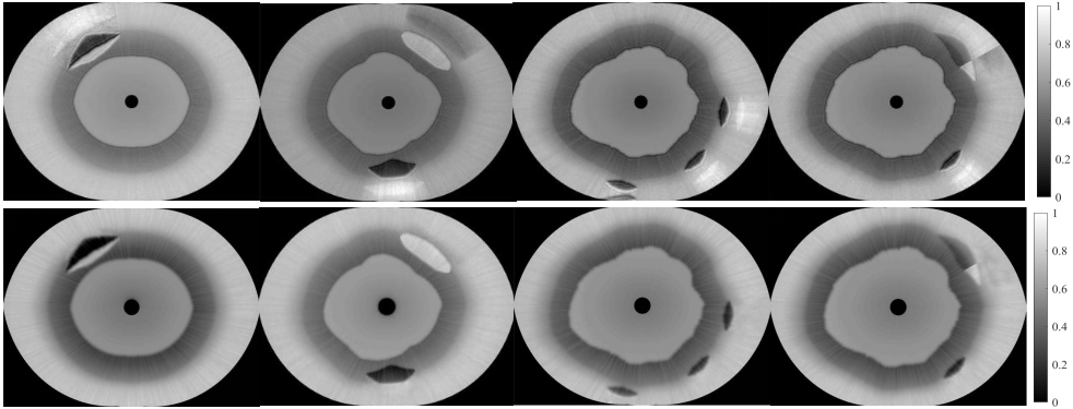
Figure 5.
Evaluation indexes of reconstructed images before and after suppression of RAs.
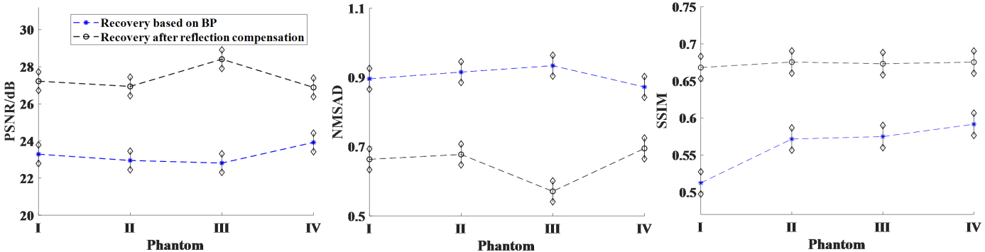
Figure 6.
Images of AOED reconstructed by SLSC (top) and CNN (bottom).
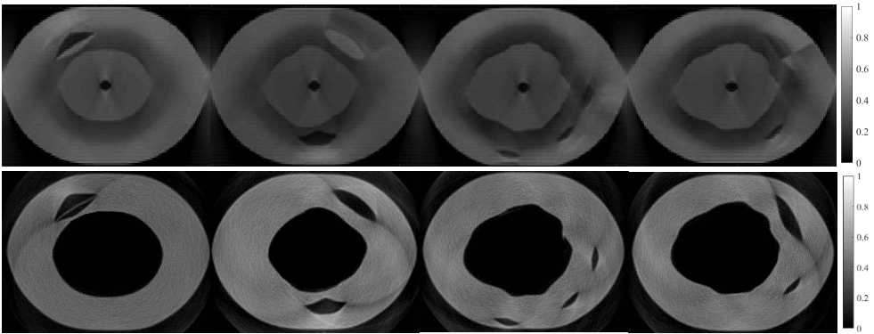
Figure 7.
Evaluation indexes of reconstructed images by using our method, SLSC and CNN.
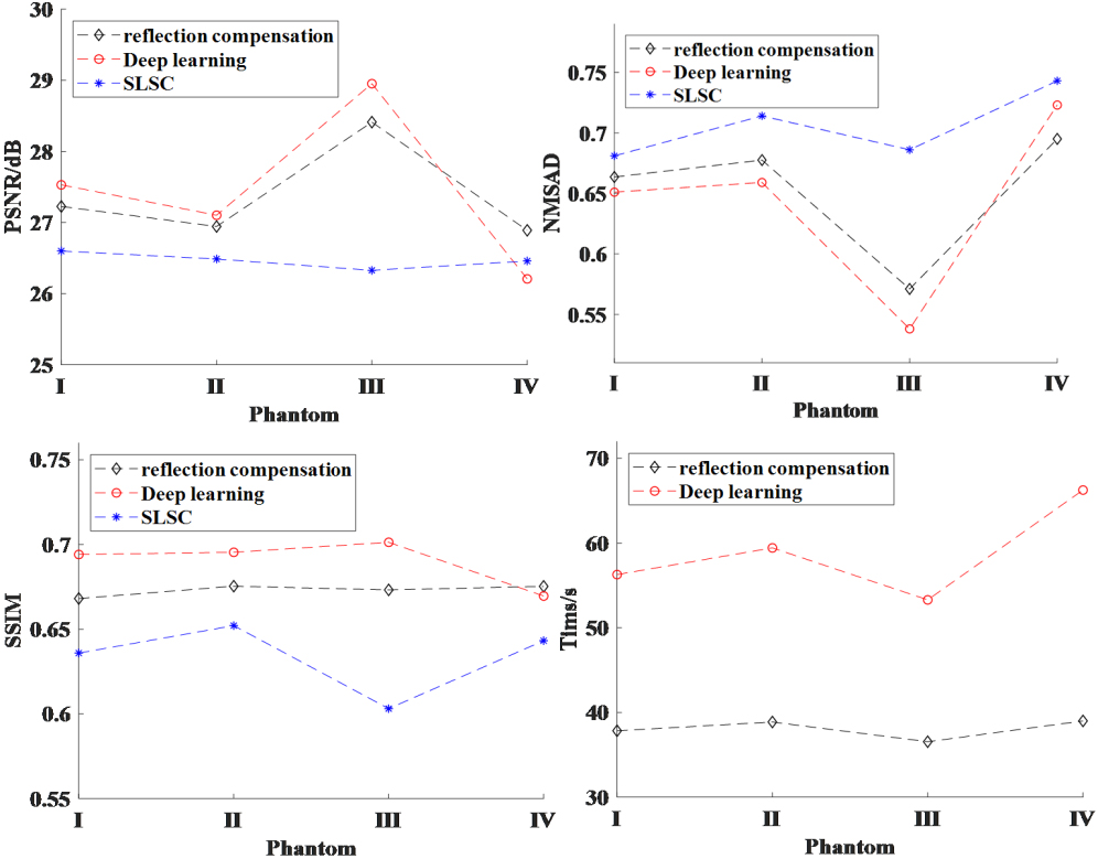
Figure 3 shows the forward simulation results of the AOED and PA signal which contains the additive Gaussian white noise with the signal-to-noise ratio (SNR) of 30 dB. The exciting wavelength and pulse duration are 1.7
Table 2
Evaluation indexes of reconstructed images in the case of
|
| Vessel phantom I | Vessel phantom II | Cavity phantom III | Cavity phantom IV | ||||||||
|---|---|---|---|---|---|---|---|---|---|---|---|---|
| PSNR (dB) | NMSAD | SSIM | PSNR (dB) | NMSAD | SSIM | PSNR (dB) | NMSAD | SSIM | PSNR (dB) | NMSAD | SSIM | |
| 0 | 26.5 | 0.678 | 0.667 | 26.8 | 0.691 | 0.660 | 26.1 | 0.720 | 0.658 | 26. 4 | 0.706 | 0.664 |
| 0.1 | 0.005 | 0.005 | 0.1 | 0.005 | 0.005 | 0.1 | 0.005 | 0.005 | 0.1 | 0.005 | 0.005 | |
|
| 27.2 | 0.663 | 0.678 | 27.5 | 0.677 | 0.677 | 28.4 | 0.572 | 0.665 | 26.9 | 0.695 | 0.672 |
| 0.1 | 0.005 | 0.005 | 0.1 | 0.005 | 0.005 | 0.1 | 0.005 | 0.005 | 0.1 | 0.005 | 0.005 | |
Figure 8.
Reconstructed images of AOED. (a) From top to bottom,
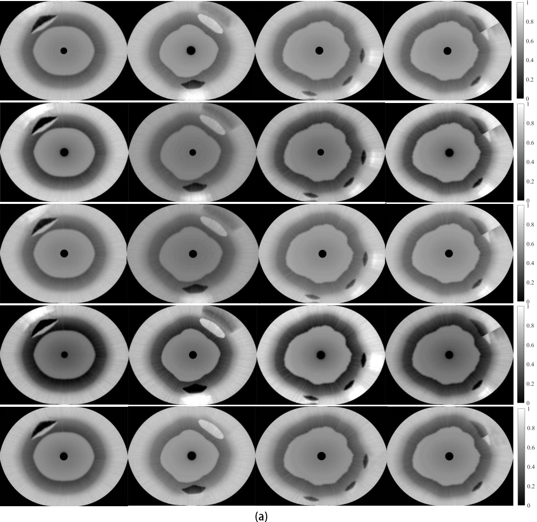
Figure 8.
Continued.
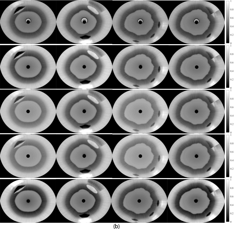
Figure 9.
Evaluation indexes of images regarding different (a)
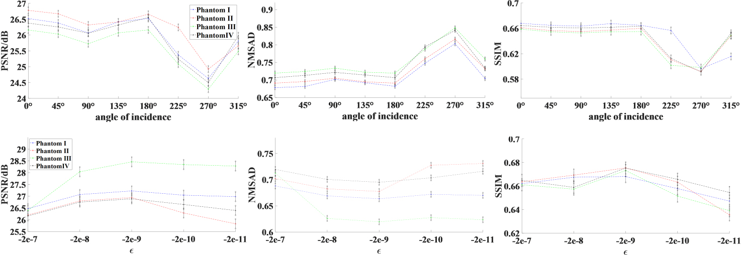
Figure 4 presents the images reconstructed by using our method and BP [15]. We utilized k-wave toolbox in MATLAB to generate the planar ultrasonic wave where
We adopted peak signal to noise ratio (PSNR), normalized mean square absolute distance (NMSAD), and structural similarity (SSIM) [17] as quantitative indices to evaluate the reconstruction quality. From Fig. 5, we concluded that the quality of the images after RA suppression is improved in comparison with that of BP reconstructions. These convincing results demonstrate the effectiveness of our method in reducing RAs and the improvement in the contrast of different tissue types.
We compared our method with the SLSC approach [8] and a CNN method of our previous work [18]. SLSC is used as a weighting factor of different signals in reconstructing images to suppress clutters and preserve PA signals as well. As stated in Introduction, the SLSC approach is unable to effectively distinguish incoherent signals generated by dense tissues from the clutters because of their similar spatial coherence. Severe artifacts are observed around the cavity wall in Fig. 6. Figure 7 reveals the improvement in the quantitative indices of our method in comparison with SLSC.
The CNN method constructs and trains a neural network based on a U-net. The network is used to optimize the time-reversal reconstructions. We constructed the data set by computer simulation which contains 5000 pairs of sample images. We trained and tested the network on a GPU configured with NVIDIA geforce 1080ti. Figures 6 and 7 reveal that the quality of CNN reconstructions is similar to that of our method. CNN has the advantages of strong learning ability and good portability. However, its performance in reconstructing high-quality images depends on the data set used for training. It can only provide application scenarios with limited amount of data, and it is time-consuming to train the network with a high requirement for hardware.
4.Discussion
We discussed the influence of the incident angle of the planar ultrasound denoted as
5.Conclusion
This work developed a method to suppress RAs in EPAT images with low requirements for equipment and operators. The results of simulated phantoms demonstrate its validity in improving the image quality. The best quality is obtained when
This study focused on removal of in-plane RAs which are produced by the acoustic scatterers and optical absorbers inside the imaging plane. As for out-of-plane reflection, a highly focused ultrasonic transducer is needed to achieve high-quality imaging, where the out-of-plane clutter can be neglected.
Deep learning has shown great potential in real-time imaging with the development of high-performance processor, big data technology, and the continuous increase of open source databases. In the future work, we plan to design a model-based strategy to suppress RAs in EPAT by combining the approximation of ideal PA signals with CNN training.
Acknowledgments
This work was supported by the National Natural Science Foundations of China (no. 62071181).
Conflict of interest
None to report.
References
[1] | Yao J, Wang LV. Recent progress in photoacoustic molecular imaging. Curr Opin Chem Biol. (2018) ; 45: : 104–112. doi: 10.1016/j.cbpa.2018.03.016. |
[2] | Ye M, Yuan J. The study of selecting the optimum SOS group based on PA imaging. J Nanjing University (Natural Sciences). (2016) ; 52: (3): 528–535. doi: 10.13232/j.cnki.jnju.2016.03.015. |
[3] | Held G, Preisser S, Akaray HG, Peeters S, Frenz M, Jaeger M. Effect of irradiation distance on image contrast in epi-optoacoustic imaging of human volunteers. Biomed Opt Express. (2014) ; 5: (11): 3765–3780. doi: 10.1364/BOE.5.003765. |
[4] | Jaeger M, Frenz M, Schweizer D. Iterative reconstruction algorithm for reduction of echo background in optoacoustic images. Proceedings of SPIE International Conference on Photons Plus Ultrasound: Imaging and Sensing 2008. San Francisco, USA; 19 Jan. (2008) . p. 68561C. doi: 10.1117/12.768822. |
[5] | Jaeger M, Harris-Birtill D, Gertsch A, O’Flynn E. Deformation compensated averaging for clutter reduction in epiphotoacoustic imaging in vivo. J Biomed Opt. (2012) ; 17: (6): 066007. doi: 10.1117/1.JBO.17.6.066007. |
[6] | Jaeger M, Bamber JC, Frenz M. Clutter elimination for deep clinical optoacoustic imaging using localised vibration tagging (LOVIT). Photoacoustics. (2013) ; 1: : 19–29. doi: 10.1016/j.pacs.2013.07.002. |
[7] | Petrosyan T, Theodorou M, Bamber J, Frenz M, Jaeger M. Rapid scanning wide-field clutter elimination in epi-optoacoustic imaging using comb LOVIT. Photoacoustics. (2018) ; 10: : 20–30. doi: 10.1016/j.pacs.2018.02.001. |
[8] | Alles EJ, Jaeger M, Bamber JC. Photoacoustic clutter reduction using short-lag spatial coherence weighted imaging. Proceedings of 2014 IEEE International Ultrasonics Symposium. Chicago, IL, USA; 3–6 Sep., (2014) . pp. 41–44. doi: 10.1109/ULTSYM.2014.0011. |
[9] | Allman D, Reiter A, Bell M. Photoacoustic source detection and reflection artifact removal enabled by deep learning. IEEE Trans Med Imaging. (2018) ; 37: : 1464–1477. doi: 10.1109/TMI.2018.2829662. |
[10] | Wang LV, Jacques SL. Monte Carlo modeling of light transport in multi-layered tissues in standard C. Houston: University of Texas M. D. Anderson Cancer Center. (1992) . |
[11] | Mohammadi L, Behnam H, Tavakkoli J, Avanaki MRN. Skull’s photoacoustic attenuation and dispersion modeling with deterministic ray-tracing: towards real-time aberration correction. Sensors. (2019) ; 19: (2): 345. doi: 10.3390/s19020345. |
[12] | La Rivière PJ, Zhang J, Anastasio MA. Image reconstruction in optoacoustic tomography for dispersive acoustic media. Opt Lett. (2006) ; 31: (6): 781–783. doi: 10.1364/OL.31.000781. |
[13] | Schiffner MF, Schmitz G. Plane wave pulse-echo ultrasound diffraction tomography with a fixed linear transducer array. Acoustical Imaging. (2012) ; 31: (3): 19–30. doi: 10.1007/978-94-007-2619-2_3. |
[14] | Singh MKA, Jaeger M, Frenz M, Steenbergen W. Photoacoustic reflection artifact reduction using photoacoustic-guided focused ultrasound: comparison between plane-wave and element-by-element synthetic backpropagation approach. Biomed Opt Express. (2017) ; 8: (4): 2245–2260. doi: 10.1364/BOE.8.002245. |
[15] | Li ML, Wang LV. A study of reconstruction in photoacoustic tomography with a focused transducer. Proceedings of SPIE International Conference on Photons Plus Ultrasound: Imaging and Sensing 2007. 13 Feb., (2007) . p. 64371E. doi: 10.1117/12.703716. |
[16] | Jacques SL. Optical properties of biological tissues: A review. Phys. Med. Biol. (2013) ; 58: (11): R37. doi: 10.1088/0031-9155/58/11/R37. |
[17] | Zhuang T. CT: Principle and Algorithm. Shanghai: Shanghai Jiao Tong University Press; (1992) . |
[18] | Sun Z, Yan X. A deep learning method for limited-view intravascular photoacoustic image reconstruction. J Med Imag Health In. (2020) ; 10: (11): 2707–2713. doi: 10.1166/jmihi.2020.3204. |
[19] | Schwab HM, Beckmann MF, Schmitz G. Photoacoustic clutter reduction by inversion of a linear scatter model using plane wave ultrasound measurements. Biomed Opt Express. (2016) ; 7: (4): 1468–1478. doi: 10.1364/BOE.7.001468. |


