Combination of variational mode decomposition and coherent factor for ultrasound computer tomography

Wang, Shanshan; Zou, Xinyi; Zeng, Liang; Song, Junjie; Zhou, Liang; Ding, Mingyue; Yuchi, Ming

doi:10.3233/THC-228016

Combination of variational mode decomposition and coherent factor for ultrasound computer tomography

Article type: Research Article

Authors: Wang, Shanshan^a | Zou, Xinyi^a | Zeng, Liang^a | Song, Junjie^b | Zhou, Liang^b | Ding, Mingyue^b | Yuchi, Ming^{b; *}

Affiliations: [a] School of Electrical and Electronic Engineering, Hubei Key Laboratory for High-efficiency Utilization of Solar Energy and Operation Control of Energy Storage System, Hubei University of Technology, Wuhan, Hubei, China | [b] School of Life Science and Technology, Huazhong University of Science and Technology, Wuhan, Hubei, China

Correspondence: [*] Corresponding author: Ming Yuchi, School of Life Science and Technology, Huazhong University of Science and Technology, Wuhan, Hubei, China. Tel.: +86 13995547537; E-mail: m.yuchi@hust.edu.cn.

Keywords: Variational mode decomposition, ultrasound computer tomography, ring array

DOI: 10.3233/THC-228016

Journal: Technology and Health Care, vol. 30, no. S1, pp. 163-171, 2022

Published: 25 February 2022

Get PDF

Abstract

BACKGROUND:

Ultrasound computed tomography (USCT) is a promising technique for improving the detection of breast cancer. Image quality of USCT has a major impact on the breast cancer diagnosis.

OBJECTIVE:

This paper investigates the combination of variational mode decomposition (VMD) and coherent factor method for USCT image quality enhancement.

METHODS:

The signals can be decomposed into multiple intrinsic mode functions (IMFs) sifting through the frequency by VMD method. Refactoring the remaining IMFs, spatio-temporally smoothed coherence factor (STSCF) beamforming method is applied to reconstructed data for USCT.

RESULTS:

The validation of combination the VMD and STSCF is described through the breast phantom experiment and in vivo experiments. The evaluation indicators such as contrast ratio (CR), contrast to noise ratio (CNR) and signal to noise ratio (SNR) have been better improved in the experimental results. For the breast phantom, the proposed method gives a higher resolution and the better contrast properties for the hyperechoic cyst. The borders of cysts and tumors in the breast phantom can be distinguished clearly. For volunteer breast experiments, artifacts are removed more efficiently while the clutters are suppressed simultaneously.

CONCLUSION:

The combination of VMD and STSCF can further reduce the noise and suppress the side lobes.

1.Introduction

Signal processing plays a crucial role in image reconstruction. Empirical Mode Decomposition (EMD) is firstly proposed in 1998 for signal decomposition, it is the core algorithm of Hilbert Huang transform (HHT) [1]. It aims at obtaining a series of intrinsic mode functions (IMF) representing the time scales of signal features by decomposing the non-linear non-stationary signals so that each IMF is a narrow-band signal for Hilbert spectrum (HS) analysis. Due to modal aliasing and endpoint effects in EMD, ensemble empirical mode decomposition (EEMD) method is proposed by Huang [2]. EEMD method overcomes the modal aliasing problem of EMD. In order to distribute the signal evenly, it adds Gaussian white noise to the signal, but there are still serious pseudo components [3, 4]. Variational mode decomposition (VMD) is an adaptive signal decomposition algorithm proposed by Dragomiretskiy and Zosso [5]. It can decompose a signal into some meaningful modes efficiently according to their frequency information and maintain good robustness. Dutta [6] points out that the VMD method decomposes data into multiple modalities to acquire and process noise signals in the data and improve the signal-to-noise ratio.

Ultrasound computed tomography (USCT) is a new management technique for breast cancer detection [7]. Image quality of USCT has a major impact on the early diagnosis of breast cancer. The raw data collected by USCT contains a lot of external noises. The effective reflection and transmission signals need to be separated from the noises. Ruiter introduced the signal pre-processing method which convolve the local maximum of the envelope with the truncated difference of the sine function [8]. Yankelevsky processed ultrasound signals by component-based modeling. It could effectively reduce the side lobe artifacts [9]. Nebojsa Duric developed a USCT system which can be reconstructed multiple images with the processing data [10].

In this work, VMD method is introduced for USCT signal processing dealing with the phase aberration of the A-scan signals. After the VMD decomposition and the remaining IMF refactoring, image reconstruction is performed by weighting with coherence factor, which can further reduce the noise and suppress the side lobes [11]. To demonstrate the benefits of the VMD method in USCT imaging, the phantom and in vivo experiments are performed.

The remainder of this paper is arranged as follows. The method of the VMD technique and the coherence factor are described in Section 2. Section 3 shows the experimental setups. The USCT system and experimental subjects are also introduced briefly. Section 4 presents the experimental results. The selection of the number of modal components are discussed in Section 5. Finally, Section 6 is devoted to the conclusion.

2.Methods

2.1Variational mode decomposition algorithm

Variational mode decomposition is a sequential process that decomposes the input signal into a discrete number of sub-signals (modes), where each mode has limited bandwidth. Each mode k has a center pulsation ωk. The number of modes can be selected which determines the center pulsation.

For assessing the bandwidth of a mode, the associated analytic signals by means of the Hilbert transform are computed so that a unilateral frequency spectrum can be obtained. By mixing with the exponent adjusted to the respective estimated center frequency, the spectrum of the mode is moved to the baseband. The constrained variational problem is described in the literature [5], the formula is given by

minuk,ωk={∑k∥∂t⁡[(δ⁢(t)+jπ⁢t)∗uk⁢(t)]⁡e-j⁢ωk⁢t∥22}

(1)

Subject to:∑kuk=f

where f the signals, uk the mode, ωk the center frequency. k number of modes, δ the Dirac distribution, t time script, and * denotes convolution. ∑k the summation over all modes.

The reconstruction constraint problem uses a quadratic penalty function and Lagrange multiplier operator. The quadratic penalty function is the method that can transform the constrained optimization problem into an unconstrained optimization problem for accurate reconstruction. Usually, prior knowledge such as Gaussian noise is added. In a noise-free environment, the weight is infinite for performing strict data fidelity, so that the processing system will show morbidity. On the other hand, the Lagrange multiplier is a method of strictly implementing constraints. The combination of the quadratic penalty function and Lagrange multiplier operator has good convergence of function under strict execution of Lagrange multipliers. The augmented Lagrangian method is as follows [12]:

(2)

L⁢(uk,ωk,λ)=α⁢∑k∥∂t⁡[(δ⁢(t)+jπ⁢t)∗uk⁢(t)]⁡e-j⁢ωk⁢t∥22+∥f⁢(t)-∑kuk⁢(t)∥22+⟨λ⁢(t),f⁢(t)-∑kuk⁢(t)⟩

where α is the balancing parameter, λ the Lagrangian multiplier. The solution method for the Eq. (2) is called the alternate direction method of multipliers (ADMM) [13]. The iterative formulas of uk and ωk are described as follow

(3)

u^kn+1⁢(ω)=f^⁢(ω)-∑i≠ku^i⁢(ω)+λ^⁢(ω)21+2⁢α⁢(ω-ωk)2

(4)

ωkn+1=∫0∞ω⁢|u^k⁢(ω)|2⁢𝑑ω∫0∞|u^k⁢(ω)|⁢d2⁢ω

where u^k⁢(ω) is the center of gravity corresponding power spectrum, f^⁢(ω) the spectrum of signal, n the number of iteration.

According to the iteration of mode uk and center frequency ωk, the ADMM algorithm is used to directly optimize in the frequency domain after Fourier transform. The update formula of Lagrangian multiplier can be obtained as follows:

(5)

λ^n+1⁢(ω)←λ^n⁢(ω)+τ⁢(f^⁢(ω)-∑ku^kn+1⁢(ω))

The final convergence formula of the mode is as follows:

(6)

∑k||u^kn+1-u^kn||⁢/.22⁢||u^kn||22<ε.

The Lagrange multiplier is to strengthen constraint, and second penalty can improve the convergence. Constraints can be relaxed using only the quadratic penalty function and deleting the Lagrangian multiplier if precise reconstruction is not required. In fact, the quadratic penalty function represents the accuracy with which the least squares are associated with the added Gaussian noise. The main process of VMD can be briefly summarized as follows [14]:

(1) Initialize u^k1, ωk1, λ^1 initial value of iteration n, maximum number of iteration N;
(2) n=n+1, update u^k for all ω⩾0 based on Eq. (3);
(3) update ωk for all ω⩾0 based on Eq. (4);
(4) update λ^ based on Eq. (5);
(5) Repeat step (2) to (4) until n>N and convergence formula ∑k||u^kn+1-u^kn||22/||u^kn||22<ε.

A complex echo signal can be decomposed into multiple modal signals by VMD. If the noise in the unexpected mode is removed and the modalities of other frequencies near the center frequency of the transducer are combined, the new data can be used to reconstruct the image.

2.2Combination of VMD and coherent factor (CF)

After the VMD decomposition, the data of the useful modality is retained. The image reconstruction is performed by weighting with coherence factor, which can further reduce the noise and suppress the side lobes.

The CF is defined as follows [15]:

(7)

C⁢F⁢[n]=|∑m=0M-1sm⁢[n]|2M⁢∑m=0M-1|sm⁢[n]|2=1-1M⁢∑m=0M-1|sm⁢[n]-s¯⁢[n]|21M⁢∑m=0M-1|sm⁢[n]|2,

where sm⁢[n] the RF data of channel m, s¯⁢[n] the mean of sm⁢[n], n the time index, |⋅| the modulus, and M the entire number of channels.

The coherent of CF is calculated at individual time index of each element. The side lobe interferences have a great influence on CF value. Spatio-temporally smoothed coherence factor (STSCF) can smooth the coherence factor spatially and temporally. It can reduce speckle variance in homogeneous regions consequently. The formula of the STSCF is

(8)

𝑆𝑇𝑆𝐶⁢F⁢[n]=∑k=-KK|∑l=0M-L∑m=lL+l-1sm⁢[n+k]|2(M-L+1)⁢∑k=-KK∑l=0M-L|∑m=lL+l-1sm⁢[n+k]|2,

where sm⁢[n+k] received RF data of channel m. K the range of time series, L is the subarray length, M the entire number of array channels.

3.Experimental setups

The experiment was carried out on the USCT system developed by the Medical Ultrasound Laboratory. The ring array consists of 1024 elements with center frequency of 2.5 MHz and sampling frequency of 12.5 MHz. The diameter of transducer is 200 mm. The ring array is placed in a suitable sink. The image object is usually placed in the center of the array and filled with water in the sink. The ring array was immersed in the sink. Water was coupled between the probe and the imaged object. Each element sequentially transmits signals, and all elements receive the echo signals. Figure 1a shows the ring transducer and breast phantom 052A (CIRSINC, USA). The phantom 052A was located in the center of the probe for scanning. Figure 1b is a data acquisition process for breast of a female volunteer. During the measurement, the volunteer was lying prostrate on the expeimental platform.

Figure 1.

(a) Ring transducer and breast phantom 052A; (b) Breast scan of a female volunteer.

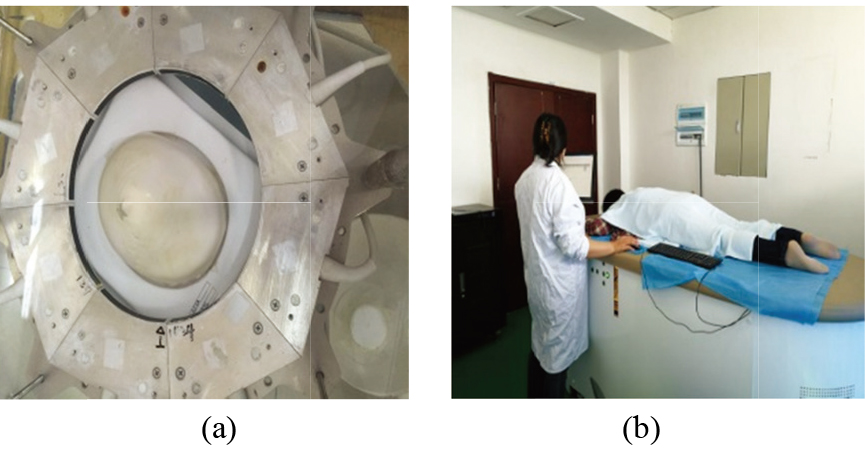
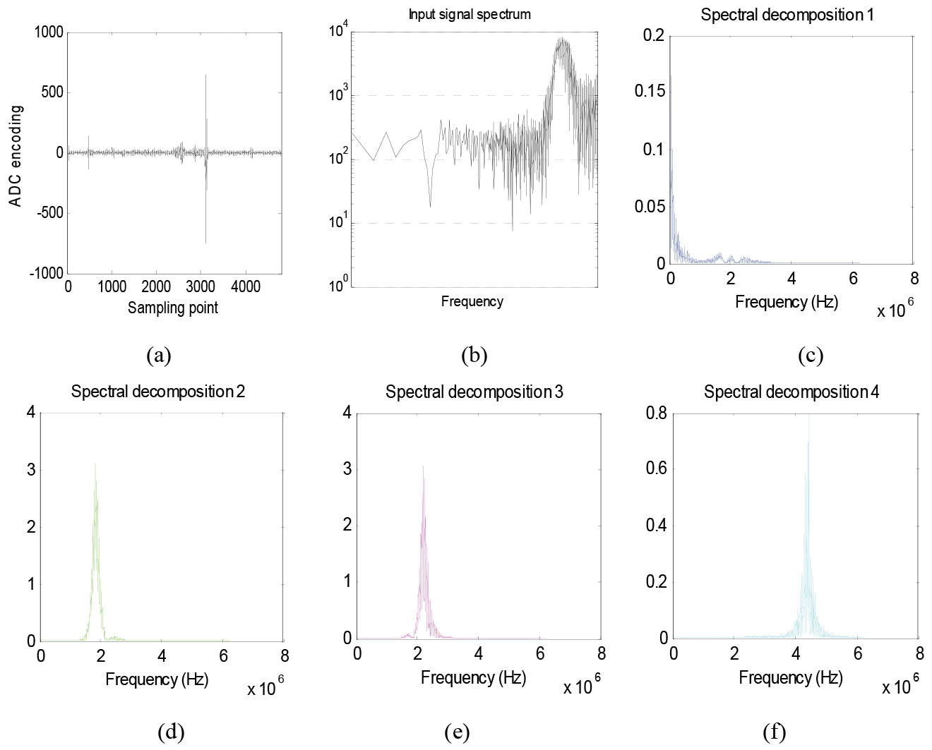
Figure 2.

The spectral analyzing for one channel data. (a) original signal; (b) spectrum of (a); (c) spectrum of mode 1; (d) spectrum of mode 2; (e) spectrum of mode 3; (f) spectrum of mode 4.

4.Experimental results

Figure 2 shows the spectral analysis of a channel data of the phantom 052A. Here, the number of k is selected as 4. Figure 2a shows the original signals of one channel in the ring array. Figure 2b shows the spectrum of the original signals. Four modes are decomposed according to the value of k. Figure 2c–f shows the spectrum of the four modal data. It can be seen that the frequency of Fig. 2c is the lowest frequency, and the Fig. 2f has the highest frequency. By performing Fourier inverse transformation on the four sets of data, time domain data of four modes can be obtained. The decomposed data can be used for imaging.

For representing the relationship between the original signal and the three modalities more clearly, the spectrum of the original signals and each mode after decomposition are plotted in logarithmic coordinates, as shown in Fig. 3. The black curve represents the original signal which is obtained by Fourier transform of the data in Fig. 2a. The blue, green, red and pale blue curves represent the spectrum of the four modes as shown in Fig. 2c–f. It can be seen from the figure that the blue part is mainly a low-frequency signal, which may be caused by the direct-current offset and need be removed. The green is a useful signal with a large value, which needs to be retained. The red part is a signal with a higher frequency, and there is also a lot of useful information. The pale blue part is the highest frequency which included lots of noises. Here, all channel signals are decomposed into four modes. The blue low-frequency mode and pale blue mode are removed, and the new data obtained by combining the other two modes is used for imaging. The imaging results are shown in Fig. 4.

Figure 3.

Spectral analyzing for one channel data and all modes.

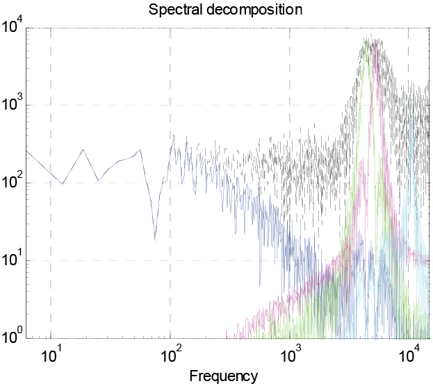
Figure 4.

Reconstructed images of breast phantom by (a) DAS; (b) VMD; (c) STSCF; (d) VMD+CF; (e) VMD+STSCF; (f) MRI.

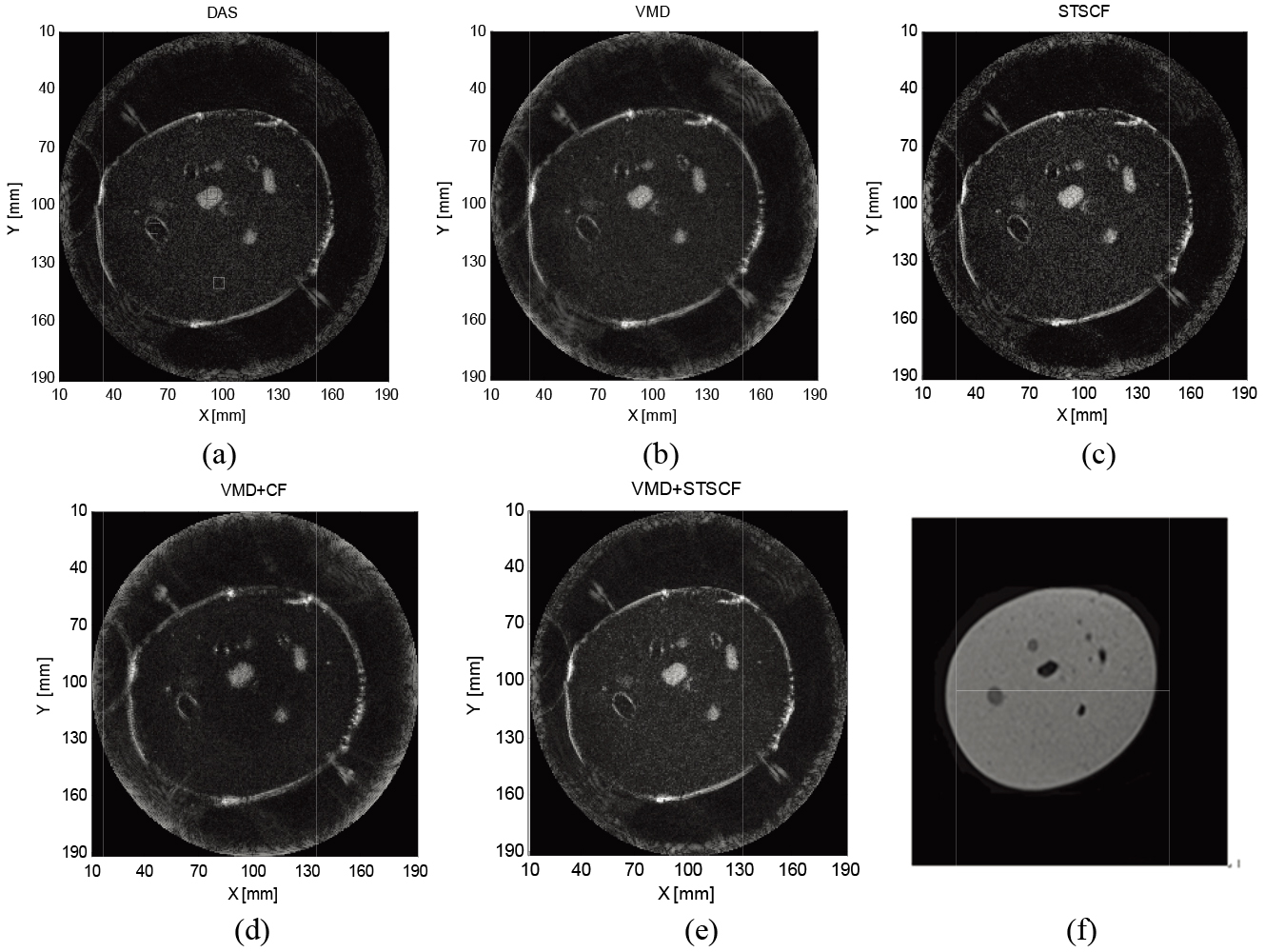
Figure 4a is the phantom 052A image reconstructed by DAS. The background is the water. Figure 4b is reconstructed by the DAS after the data processing using VMD method. Mode 2 and mode 3 data are remained for reconstructed. The image reconstructed by VMD method has higher contrast while the cysts and calcification points in the phantom are clearer compared with DAS. But the artifacts in the water are also clearer. Figure 4c is reconstructed using traditional DAS beamformer weighted by the STSCF. Figure 4d is reconstructed using the CF method weighted combination of the remaining mode 2 and mode 3 data using VMD decomposition. In Fig. 4e, the CF method is replaced by the STSCF method for reconstructed images. Figure 4f shows the image by MRI scanning.

For quantity analysis, CR, CNR and SNR were calculated to evaluate image contrast and resolution. Table 1 shows the values of CR, CNR and SNR before and after processing by the VMD method. CR is defined as C⁢R=|μ𝑅𝑂𝐼-μB|. μB and μ𝑅𝑂𝐼 are the mean value of the background and region-of-interest (ROI) respectively. CNR is defined as the ratio of CR to σB. σB is the standard deviation of amplitudes in the background [16]. SNR is calculated as 𝑆𝑁𝑅=μB⁢/.⁢σB.

Table 1

CR, CNR and SNR of different methods for the breast phantom

Method	CR	CNR	CR	CNR	Mean	Std	SNR
	ROI1		ROI2		Background
DAS	0.96	0.09	88.38	8.01	28.57	11.04	0.54
VMD	1.01	0.13	99.53	13.03	33.35	7.64	0.84
STSCF	1.31	0.09	120.01	8.25	32.15	10.54	0.34
VMD-CF	0.98	0.09	75.39	11.38	29.31	6.62	0.94
VMD-STSCF	1.38	0.16	123.79	13.79	38.01	8.25	0.65

In ROI1, using the VMD method can increase CR from 0.96 dB to 1.01 dB compared with DAS. In ROI2, the CR is increased from 88.38 dB to 99.53 dB. Using the VMD+STSCF method, the CR is further improved. Therefore, both in the hyperechoic area and the hypoechoic area, the method can effectively improve the contrast. Similarly, CNR is also increased by 0.04 dB to 5 dB. The uniform tissue in the phantom is selected as the background region, the mean value of the region and the overall brightness of the image increase a little. The background variance became smaller which indicated that the tissue image in the phantom appeared to be more uniform using VMD method. In the reconstruction of the VMD method, the image quality of the phantom is improved but more artifacts can be seen in the water. It shows that this method will still lead to the generation of pseudo components when data decomposition is performed, but the main influence is the near field data.

When VMD is combined with CF, the contrast of ROI1 is slightly improved, and the contrast of ROI2 is decreased. This indicates that after the VMD processing, the CF method can suppress the side lobes and improve the contrast in the low echo region, but at the same time it also produces a serious pseudo. Due to the influence of artifacts, the contrast is reduced in the high echo region. At the same time, there are black artifacts around the middle high echo area of the ring. When VMD is combined with STSCF, the CR and CNR of both ROI regions are improved. Compared with the use of the VMD method alone, or the use of the STSCF method alone as shown in Fig. 4, the combination of the two methods can better reduce the side lobes and clutter.

Figure 5.

Reconstructed images of female volunteer breast by (a) DAS; (b) VMD; (c) VMD+CF; (d) VMD+STSCF.

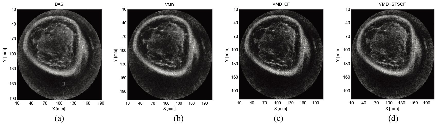
Figure 5a is the breast image of a female volunteer reconstructed by DAS, and Fig. 5b is reconstructed after the data processing using VMD method. It can be seen that compared with DAS, the contrast is higher using the VMD method. Figure 5c is reconstructed by CF combined with VMD method. Figure 5d is STSCF combined with VMD. Table 2 shows the CR, CNR and SNR values before and after processing with the VMD method. The CR is increased from 0.5 dB to 6.49 dB. In ROI2, the CR is increased from 11.43 dB to 13.68 dB. Therefore, in the high echo region and the low echo region, the method can effectively improve the contrast. Similarly, the CNR has also increased by 0.4 dB. A more uniform portion of the image of the water is selected as the background, the brightness and the variance are reduced. The background appears to be more uniform. When VMD is combined with CF, the contrast of ROI1 is slightly higher than that of DAS, and the contrast of ROI2 is decreased. This indicates that after the VMD processing of the data, the CF method can suppress the side lobes and improve the contrast in the low echo region. However, at the same time, it also produces artifacts. Because of the effects of artifacts, the contrast is reduced in the hyperechoic area. When VMD is combined with STSCF, the CR and CNR of the two ROI regions are improved. Compared with the VMD method alone, the combination of the two methods can better reduce the side lobes and clutter.

Table 2

CR, CNR and SNR of different methods

Method	CR	CNR	CR	CNR	Mean	Std	SNR
	ROI1		ROI2		Background
DAS	0.50	0.03	11.43	0.59	58.24	19.51	0.28
VMD	1.19	0.04	13.68	0.92	39.15	14.86	0.28
VMD-CF	0.56	0.02	7.91	0.42	68.75	18.81	0.22
VMD-STSCF	1.21	0.06	9.52	0.46	47.91	20.76	0.23

5.Discussion

Before the VMD applied, the number of modal components k needs to be determined. The k value affects the center frequency of each modal component after decomposition. A bigger k means more modes can be decomposed, and which is supposed to obtain more modal combination patterns. However, there has been a phenomenon of over-decomposition of the center frequency. In this paper, k is determined by observing the center frequency of each modal component. Using VMD method to decompose the data in Fig. 2a. All modes k are shown in Table 3.

Table 3

Center frequency corresponding to different k

Number k	Center frequency (/MHz)
2	0.06	1.94	–	–	–	–	–
3	0.06	1.94	4.09	–	–	–	–
4	0.06	1.85	2.19	4.45	–	–	–
5	0.06	1.81	2.08	2.45	4.91	–	–
6	0.06	1.81	2.08	2.45	4.16	4.91

In Table 3, over-decomposition of the center frequency appeared when k is selected as 5. Here, we assumed k= 4.

6.Conclusion

The input data can be modulated adaptively by VMD method which can avoid modal aliasing and pseudo component generation effectively. Meanwhile, the method represents the original signal at a good scale and reduces noise interference. However, this method also has some problems, such as artifacts may increase and affect the near field data. STSCF can smooth CF both spatially and temporally, reducing the impact of CF changes and improving image quality effectively. The combination of VMD and STSCF can further reduce the noise and suppress the side lobes. The results of the breast phantom and volunteer breast experiments show that it can effectively reduce noise while reducing side lobes compared with the traditional imaging method.

Acknowledgments

This research was supported by the National Key R&D Program of China (2016YFE0203900, 2018YFC0116100) and the Hubei University of Technology Doctoral Research Startup Fund Project (BSQD2019018).

Conflict of interest

None to report.

References

[1]	Huang HE, Shen Z, Long SR, Wu MC, The empirical mode decomposition and the Hilbert spectrum for nonlinear and nonstationary time series analysis, The Royal Society. (1998) ; 454: (1971): 903–993.
[2]	Wu Z, Huang HE, Ensemble empirical mode decomposition: A noise-assisted data analysis method, Adv. Adapt. Data Anal. (2008) ; 1: (1): 1–40.
[3]	Guo CW, Ding Y, Yuan J, Xu G, Wang XD, Carson PL, Adaptive photoacoustic imaging quality optimization with EMD and reconstruction, SPIE Medical Imaging. (2016) ; 10024.
[4]	Liao A, Shen C, Li P, Potential Contrast Improvement in Ultrasound Pulse Inversion Imaging Using EMD and EEMD, IEEE trans. Ultrason. Ferroelectr. Freq. Control. (2010) ; 57: (2): 317–326.
[5]	Dragomiretskiy K, Zosso D, Variational mode decomposition, IEEE Trans. on Signal Processing. (2014) ; 62: (3): 531–544.
[6]	Dutta T, Satija U, Ramkumar B, A novel method for automatic modulation classification under non-Gaussian noise based on variational mode decomposition, Communication. (2016) ; 1: : 1–8.
[7]	Duric N, Littrup P, Roy O, Li CP, Schmidt S, Cheng XY, Janer R, Clinical breast imaging with ultrasound tomography: A description of the SoftVue system, J. Acoust. Soc. Am. (2014) ; 135: : 2155–2155.
[8]	Ruiter NV, Schwarzenberg GF, Zapf M, Improvement of 3D Ultrasound Computer Tomography Images by Signal Pre-Processing. IEEE Ultrason. Symp. (2008) ; 852–855.
[9]	Yankelevsky Y, Friedman Z, Feuer A, Component-based modeling and processing of medical ultrasound signals, IEEE trans. Ultrason. Ferroelectr. Freq. Control. (2017) ; 65: (21): 5743–5755.
[10]	Duric N, Littrup P, Roy O, Clinical breast imaging with ultrasound tomography: A description of the SoftVue system. J. Acoust. Soc. Am. (2014) ; 135: (4): 2155–2155.
[11]	Wang SS, Zeng L, Song JJ, Zhou L, Coherence Factor-Like beamforming for ultrasound computed tomography, Journal of Medical Imaging and Health Informatics. (2020) ; 10: (1): 672–676.
[12]	Bertsekas DP, Multiplier methods: A survey, Automatica. (1976) ; 12: (2): 133–145.
[13]	Hestenes MR, Multiplier and gradient methods, J. Optimiz. Theory Appl. (1969) ; 4: (5): 303–320.
[14]	Fu WL, Zhou JZ, Zhang YC, Fault diagnosis for rolling element bearings with VMD time-frequency analysis and SVM, Fifth International Conference on Instrumentation and Measurement, Computer, Communication and Control. (2015) ; 69–72.
[15]	Nilsen CC, Holm S, Wiener beamforming and the coherence factor in ultrasound imaging, IEEE trans. Ultrason. Ferroelectr. Freq. Control. (2010) ; 57: : 1329–1346.
[16]	Lediju M, Trahey GE, Byram BC, Dahl JJ, Short-lag spatial coherence of backscattered echoes: Imaging characteristics, IEEE trans. Ultrason. Ferroelectr. Freq. Control. (2011) ; 58: : 1377–1388.