
3D segmentation of lungs with juxta-pleural tumor using the improved active shape model approach
Abstract
BACKGROUND AND OBJECTIVE:
At present, there are many methods for pathological lung segmentation. However, there are still two unresolved problems. (1) The search steps in traditional ASM is a least square optimization method, which is sensitive to outlier marker points, and it makes the profile update to the transition area in the middle of normal lung tissue and tumor rather than a true lung contour. (2) If the noise images exist in the training dataset, the corrected shape model cannot be constructed.
METHODS:
To solve the first problem, we proposed a new ASM algorithm. Firstly, we detected these outlier marker points by a distance method, and then the different searching functions to the abnormal and normal marker points are applied. To solve the second problem, robust principal component analysis (RPCA) of low rank theory can remove noise, so the proposed method combines RPCA instead of PCA with ASM to solve this problem. Low rank decompose for marker points matrix of training dataset and covariance matrix of PCA will be done before segmentation using ASM.
RESULTS:
Using the proposed method to segment 122 lung images with juxta-pleural tumors of EMPIRE10 database, got the overlap rate with the gold standard as 94.5%. While the accuracy of ASM based on PCA is only 69.5%.
CONCLUSIONS:
The results showed that when the noise sample is contained in the training sample set, a good segmentation result for the lungs with juxta-pleural tumors can be obtained by the ASM based on RPCA.
1.Introduction
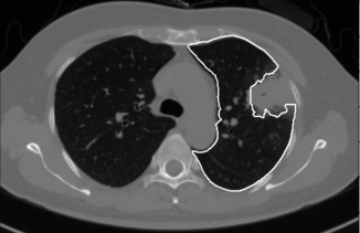
Pulmonary parenchyma segmentation is the first step in computer-aided diagnosis of lung cancer. The segmentation methods of pulmonary parenchyma which includes normal and pathological can be divided into three categories, that is based on visual appearance [1], the location relationship of shape [2] and hybrid [3]. The first kind of methods mostly considers that the gray value of lung area is lower than that of other surrounding tissues, so the pathological lung (especially including interstitial lung disease) is segmented by classifier based on gray and texture features. However, such methods are only suitable for the pulmonary segmentation of no juxta-pleural tumor, because the small different of gray value between pleura and tumor, as shown in Fig. 1. The second kind of methods mainly introduces the anatomical relationship between lung and heart, liver, spleen, rib. But this method still cannot solve the problem that is juxta-pleural tumor is excluded into the pulmonary parenchyma. The third kind of methods establishes shape model and evolves lung contour according to the surface features. Sun et al. [4] used Active Shape Model (ASM) to obtain the initial lung contour, and then used local surface features to drive the evolution of contour. Anthimopoulos et al. [5] used 15 lung image sequences to construct probability map of normal lung regions, and used registration method to segment pathological lung. Alam et al. [6] used marker points on ribs and spines to initialize the shape model, and then combined with deformable models to segment lung regions with large tumors. The above literatures can achieve better segmentation results without noise samples in training set, however they all do not consider the problem of noise samples in training set during the construction process of the training shape model. Noise samples are the images in training dataset which have incorrect contours, such as Fig. 1.
Figure 1.
Lung segmentation result is marked by white contour. This lung with a large juxta-pleural tumor is segmented by the traditional method.
When the juxta-pleural tumor’s diameter is less than 3 cm, they can be filled by morphological or curved surface fitting methods. However, when the juxta-pleural tumor’s diameter is larger than 3 cm, it needs a segmentation algorithm which can consider both the prior shape and the features of the image to be segmented. ASM is such a segmentation algorithm [7].
ASM expresses the shape model based on point distribution model (PDM). The shape model uses principal component analysis (PCA) to learn the average shape and deformation range according to the training set. And then ASM establishes the local feature appearance model according to the training set. Finally, ASM evolves the contour of the test image based on local feature appearance model and the shape model. However, PCA used in ASM can only remove the influence of noise samples which obey Gaussian distribution. That is to say, when there are other type noise samples in the training set, ASM cannot train the correct shape model. Moreover, the segmentation effect of ASM is also affected by abnormal marker points that located on pseudo-edges [8].
In recent years, scholars have applied low rank theory to image shape processing, including alignment and segmentation. In the study by Zhou et al. [9], the low rank theory is applied to the non-rigid alignment of image sets. Ahmedtl et al. [10] propose a fixed deformable face set alignment algorithm, which combines low rank theory and piecewise affine transformation into the alignment model. Li et al. [11] combined low rank and Active Appearance Model. Hu et al. [12] and Zhang et al. [13] proposed sparse shape composition (SSC) based on sparse theory and applied it to liver shape modeling. The above literatures had solved the problem of non-Gaussian noise sensitivity in shape model and all achieved good results. However, the low rank theory has not yet been applied to the ASM model.
Scholars have also done a lot of research in abnormal marker point detection. If the updated distance offset of a marker point is bigger than other marker points, the marker point is an abnormal marker point. Shi et al. and Shao et al. [14, 15] randomly divides the set of marker points into several subsets. If the shape reconstructed by the subset of marker points is different from the shape reconstructed by the corresponding marker points according to the training model, it shows that this subset contains abnormal marker points.
The shapes of training sample set have low rank attribute because the lung anatomical shape of different human is roughly same. Robust principal component analysis (RPCA) in low rank theory is more robust to noise samples. Therefore, this paper combined RPCA with ASM to solve the problem that the correct shape model cannot be obtained because of the noise samples in the training set. In the process of evolving lung boundary contour, some marker points called abnormal marker points cannot be updated to the real edge, so it is necessary to identify these abnormal marker points first. In this paper an abnormal marker point recognition method based on distance threshold is designed and assigns different searching functions to abnormal and normal marker points. For abnormal marker points, only the prior shape model is considered in searching functions while for normal marker point local low level features appearance model and shape model should also be considered together.
Figure 2.
The flow chart of the proposed algorithm.
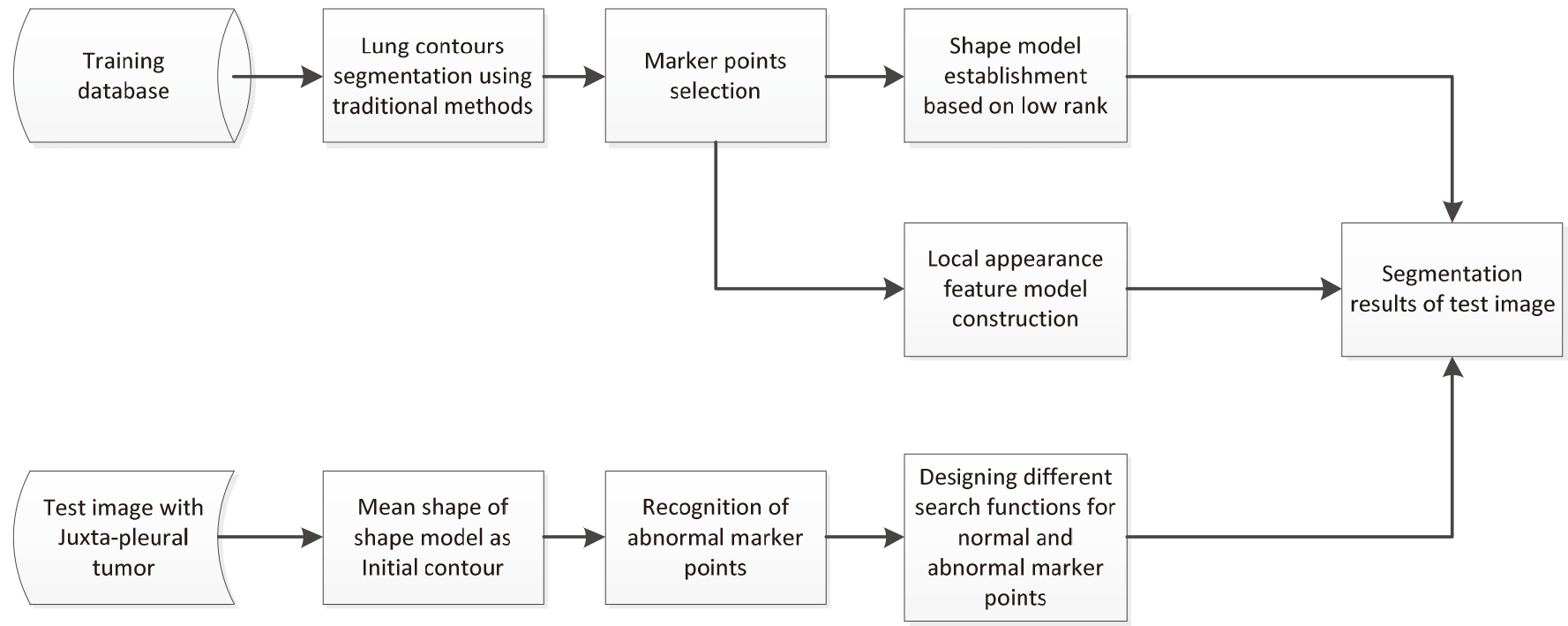
The flowchart of the proposed algorithm is shown in Fig. 2, including training and testing phase. In the training phase first use traditional segmentation methods to obtain lung contours of training data set. Then select marker points on the segmented lung contour. At last construct two models: shape model based on low rank and local appearance feature model. In the testing phase, mean shape of training data set’s shape model is considered as the initial contour of ASM. Then use traditional segmentation methods to obtain the pseudo-contour which always excludes juxta-pleural tumor. Select marker points on the pseudo-contour. Distinguish normal and abnormal marker points. Design different searching functions for normal and abnormal marker points. Subsequently, the initial shape is iteratively deformed and refined by different searching functions under training dataset’s shape model and local appearance feature model.
2.Lung with juxta-pleural tumor segmentation method
2.1Marker points extraction
First, the traditional method is used to segment the pulmonary region of the samples in training set and obtained lung boundary contour. The segmentation steps include extra-pulmonary region exclusion by iteration threshold and region growing segmentation methods, trachea elimination, internal cavity filling, liver exclusion and left and right lungs separation [16].
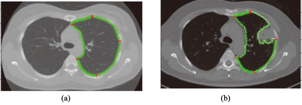
Second, extract marker points on left or right lung boundary contour, respectively according to Shenshen et al. [17]. In this way, there are 5 main marker points and 90 marker points in the left or right lung boundary (as shown in Fig. 3).
Figure 3.
Extracted marker points. Main marker points are shown in red; other marker points are shown in green. (a) normal lung (b) pathological lungs with juxta-pleural tumor.
2.2Shape model established
Aligned lung boundaries in training sample dataset by procrustes analysis method. In order to remove the influence of the noise contours such as Fig. 3b, PCA is replaced by RPCA.
The boundary contours of images in the training data set is
Firstly,
(1)
where
(2)
where
(3)
where
(4)
where
(5)
Equation (2.2) can be written in the form of Eq. (6). The accelerated approximation gradient [18] is used to solve Eq. (6).
(6)
Calculating the eigenvalues of
Figure 4.
The mean shape
2.3Model solution
The accelerated approximation gradient [18] is used to solve Eq. (2.2).
| 1: Input: |
| 2: |
| 3: While no convergence |
| 4: |
| 5: |
| 6: |
| 7: |
| 8: |
| 9: |
| 10: |
| 11: End while |
| 12: Output: |
The accelerated approximation gradient [18] is used to solve Eq. (2.5.2).
| 1: Input: |
| 2: |
| 3: While not convergence |
| 4: |
| 5: |
| 6: |
| 7: |
| 8: |
| 9: |
| 10: |
| 11: End while |
| 12: Output: |
2.4Local appearance feature model construction
In this paper, a local appearance feature model is established based on PCA using gray features. The gray-level appearance model that describes the typical image structure around each marker point is obtained from pixel profiles, sampled (using linear interpolation) around each marker point, perpendicular to the boundary contour. On either side
For each marker point
2.5Target contour search
2.5.1Recognition of abnormal marker point
Because of the adhesion between tumor and chest wall, concave lung contour is obtained based on the traditional ASM method, as shown in Fig. 5 in blue. The marker points on the contour notch are the abnormal marker points. These abnormal marker points are updated to the boundary between lung parenchyma and tumor. Therefore, the different search function of abnormal marker points should be given for abnormal marker points.
Firstly, lung contour with juxta-pleural tumor
the alignment results are shown in Fig. 5.
Figure 5.
Align the mean contour of the training samples which is shown in red and lung contour with juxta-pleural tumor which is shown in blue.
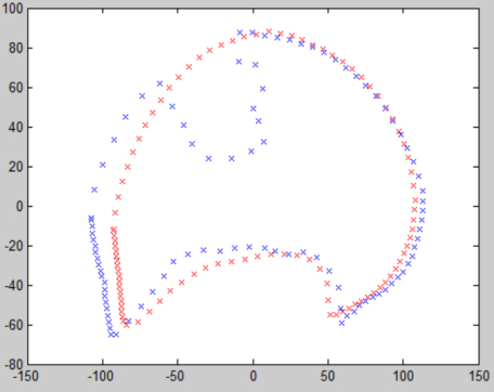
Figure 6.
The corresponding points distance between the lung contour with juxta-pleural tumor and the mean contour of the training samples.
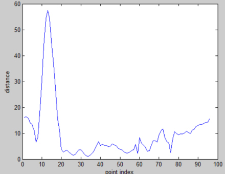
If the distance of the corresponding marker point between the lung contour with juxta-pleural tumor and the mean contour of the training samples is bigger than the threshold value
2.5.2Search the targeted contour
The initial searching curve is the mean contour. Then defines the searching rule by piecewise function. For abnormal marker point, should only make b in the range of
(7)
3.Experiment
3.1Experiment data set
First, the training dataset is established. The training dataset consists of 135 multi-slice spiral CT lung scan images collected from the First Affiliated Hospital of Guangzhou Medical University. And among them, sixteen scans are included juxta-pleural tumor on the left side and fourteen scans are included juxta-pleural tumor on the right side. The size of the lung scan images is 512*512*100
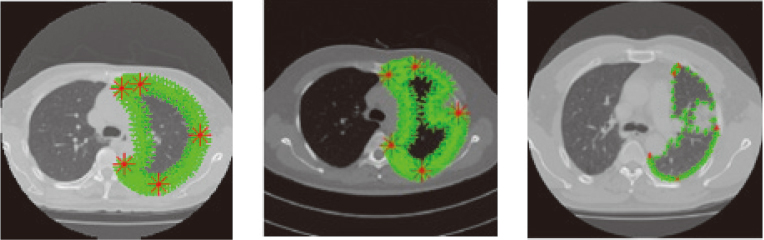
Figure 7.
Training samples including noise samples, the five main marking points are red, the marking points are green. (a) marker points in lung contour with no juxta-pleural tumor. (b) and (c) marker points in lung contour with juxta-pleural tumor.
3.2Parameter setting
In low rank algorithm,
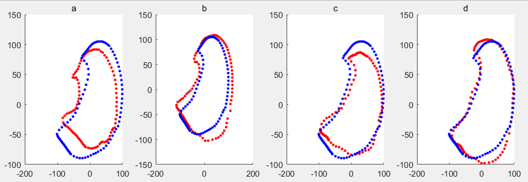
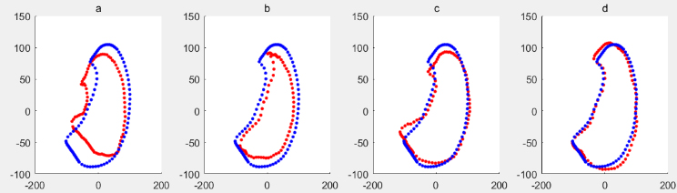
Figure 8.
Mean shape of training sample set including noise samples is shown in blue, the deformed shape based on RPCA of ASM is shown in red, when
![Mean shape of training sample set including noise samples is shown in blue, the deformed shape based on RPCA of ASM is shown in red, when t=1∼4 respectively. The shape model is shown in Fig. 9 using ASM of PCA for the training data set with noise samples. The code of traditional ASM was used [7].](https://ip.ios.semcs.net:443/media/thc/2021/29-S1/thc-29-S1-thc218037/thc-29-thc218037-g008.jpg)
3.3Comparisons of generated shape models
The shape model is shown in Fig. 8 using ASM of RPCA for the training data set with noise samples. It can be seen that the larger t is, the more similar the shape obtained is to the average shape. And the code of low rank was also used [20]. The shape model is shown in Fig. 10 using ASM of PCA for the training data set without noise samples. When
Figure 9.
Mean shape of training sample set including noise samples is shown in blue, the deformed shape based on PCA of ASM is shown in red, when
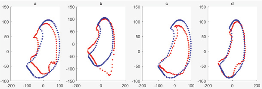
Figure 10.
Mean shape of training sample set without noise samples is shown in blue, the deformed shape based on PCA of ASM is shown in red, when
3.4Evaluation of segmentation results
The contour containment region obtained by the segmentation algorithm is compared with the contour containment region manually drawn by the doctor (as the golden standard), and the coverage degree overlap is calculated.
(8)
While
Table 1
TPF of three situations comparison
| ASM | ASM | ASM | |
|---|---|---|---|
| Left lung | 97.79 | 76.79 | 95.00 |
| Rightlung | 96.89 | 78.60 | 93.54 |
Table 2
Relationship between noise samples’ number and accuracy for RPCA
| 4 | 8 | 12 | 14/16 | |
|---|---|---|---|---|
| Left lung | 97.54% | 97.12% | 96.68% | 95.03% |
| Rightlung | 96.12% | 95.73% | 94.69% | 93.54% |
![The result of lung segmentation. (a) [15]’s method (b) ASM based on RPCA.](https://ip.ios.semcs.net:443/media/thc/2021/29-S1/thc-29-S1-thc218037/thc-29-thc218037-g011.jpg)
Figure 12.
Lung segmentation processing with juxta-pleural tumor by the ASM based on RPCA.
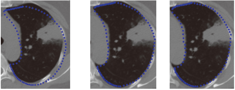
Figure 13.
Compares the lung segmentation results with juxta-pleural tumor based on ASM based on PCA and ASM based on RPCA; (a)
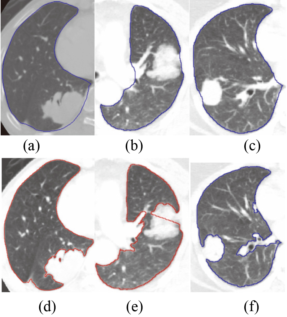
Figure 14.
Lung segmentation result with tumor by ASM based on RPCA.
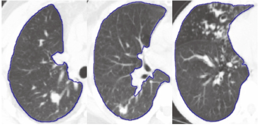
Figure 15.
3D visualization results. (a) ASM based on PCA; (b) ASM based on RPCA.
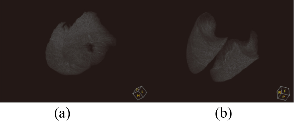
The segmentation results were compared with the ground truth according to TPF (true positive fraction) under three situations, shown as Table 1. The first situation is the train dataset doesn’t contain noise samples and using traditional ASM; the second situation is the train dataset includes noise samples and using traditional ASM; the third situation is the train dataset includes noise samples and using RPCA-based ASM. From Table 1, it can be seen that RPCA-based ASM is largely unaffected by the training set noise images. The relationship between noise samples’ number in the training dataset and segmentation accuracy for RPCA-based ASM is shown in Table 2. It can be seen that with the increase of the number of noise samples, the accuracy of segmentation is decreasing. Figure 12 shows the initial position, middle position and final position of the lung contour searching process by the proposed method. Figure 13 compares the ASM based on RPCA and traditional ASM method in lung segmentation with juxta-pleural tumor. It can be seen that the proposed method is also useful for large juxta-pleural tumors. Figure 14 shows the effect of the lung segmentation with tumor by the ASM based on RPCA. Figure 15 shows 3D visualization results of ASM based on PCA and ASM based on RPCA. In 3D visualization results, ASM based on PCA cannot include juxta-pleural tumors into the lung parenchyma, so a hole is shown.
3.5Computer time
The proposed algorithm was implemented in C++ and Matlab Lib and test on a PC with Intel i7-8550U CPU and 8GB of RAM. The average computing time of the algorithm was 5
4.Conclusion
When using ASM based on PCA to segment lung region, the correct shape model cannot be obtained under the training data set with noise samples. In this paper, we combined the RPCA based on the low rank theory which can remove the influence of noise samples on the shape model. The average overlap degree of ASM segmentation based on RPCA is 94.5%, while the average overlap degree of traditional ASM segmentation based on PCA is 69.5%, under the training data set with the noise samples. Experiments show that ASM based on RPCA can achieve better segmentation results than traditional ASM.
The search step of traditional ASM is a least square optimization method, which is sensitive to outlier marker points. Because the CT gray value of the juxta-pleural tumor is similar to lung wall, some marker points are likely to be updated to the transition region of normal lung tissues and tumor rather than the real lung border in the searching process, so it is necessary to identify these abnormal markers firstly. A new abnormal marker identification method is proposed and give different searching function for normal markers and abnormal markers. Experiments show the improved ASM method can get better results than the traditional one. With the results obtained in this work, future endeavor will research the different type pathological lung segmentation framework into a lung CAD system.
Acknowledgments
This work was financially supported by the Natural Science Foundation of China (61703285), the China Postdoctoral Science Foundation (2019M651142), the Liaoning Province Universities Scientific Research Project (20180550615), and the Shenyang Science and Technology Plan Project (18013015).
Conflict of interest
None to report.
References
[1] | Gu Y, Lu X, Yang L, et al. Automatic lung nodule detection using a 3D deep convolutional neural network combined with a multi-scale prediction strategy in chest CTs. Computers in Biology and Medicine. (2018) ; 103: : 220-231. |
[2] | Oluyide OM, Jules-Raymond T, Serestina V. Automatic lung segmentation based on Graph Cut using a distance-constrained energy. IET Computer Vision. (2018) ; 12: (5): 609-615. |
[3] | Sharif MI, Li JP, Naz J, et al. A comprehensive review on multi-organs tumor detection based on machine learning. Pattern Recognition Letters. (2020) ; 131: : 30-37. |
[4] | Sun S, Bauer C, Beichel R. Automated 3-D Segmentation of Lungs with Lung Cancer in CT Data Using a Novel Robust Active Shape Model Approach. IEEE Transactions on Medical Imaging, (2012) . |
[5] | Anthimopoulos M, Christodoulidis S, Ebner L, et al. Semantic segmentation of pathological lung tissue with dilated fully convolutional networks. IEEE Journal of Biomedical and Health Informatics. (2018) ; 23: (2): 714-722. |
[6] | Alam J, Alam S, Hossan A. Multi-stage lung cancer detection and prediction using multi-class svm classifie[C]//2018 International Conference on Computer, Communication, Chemical, Material and Electronic Engineering (IC4ME2). IEEE, (2018) ; 1-4. |
[7] | Ginneken B. et al. Active Shape Model Segmentation with Optimal Features, IEEE Transactions on Medical Imaging, (2002) . |
[8] | Zhou X, Yu W. Low-rank modeling and its applications in medical image analysis[C]// SPIE Defense, Security, and Sensing. International Society for Optics and Photonics, (2013) . |
[9] | Zhou X, Yang C, Zhao H, et al. Low-Rank Modeling and Its Applications in Image Analysis. ACM Computing Surveys. (2014) ; 47: (2): 1-33. |
[10] | Ahmedtl J, Gao B, Woo WL, et al. Ensemble Joint Sparse Low Rank Matrix Decomposition for Thermography Diagnosis System. IEEE Transactions on Industrial Electronics, (2020) . |
[11] | Li A, Chen D, Wu Z, et al. Self-supervised sparse coding scheme for image classification based on low rank representation. PloS One. (2018) ; 13: (6): e0199141. |
[12] | Hu Z, Nie F, Tian L, et al. A comprehensive survey for low rank regularization. arXiv preprint arXiv1808.04521, (2018) . |
[13] | Zhang S, Zhan Y, Dewan M, et al. Towards robust and effective shape modeling Sparse shape composition. Medical Image Analysis. (2012) ; 16: (1): 265-277. |
[14] | Shi C, Cheng Y, Wang J, et al. Low-rank and sparse decomposition based shape model and probabilistic atlas for automatic pathological organ segmentation. Medical Image Analysis. (2017) ; 38: : 30-49. |
[15] | Shao YQ, Gao YZ, Guo YR, Shi YH, Yang X, Shen DG. Hierarchical lung field segmentation with joint shape and appearance sparse learning. IEEE Transactions on Medical Imaging. (2014) ; 33: (9): 1761-1780. |
[16] | Hu S, Hoffman EA, Reinhardt TJM. Automatic lung segmentation for accurate quantitation of volumetric X-ray CT images. IEEE Trans Med Imaging. (2001) ; 20: (6): 490-498. |
[17] | Sun S, Ren H, Meng F. Abnormal lung regions segmentation method based on improved ASM, 2016 Chinese Control and Decision Conference (CCDC), (2016) . |
[18] | Jin C, Netrapalli P, Jordan MI. Accelerated gradient descent escapes saddle points faster than gradient descent[C]//Conference on Learning Theory. PMLR, (2018) ; 1042-1085. |
[19] | Murphy K, van Ginneken, et al. Evaluation of registration methods on thoracic CT: the EMPIRE10 challenge. IEEE Trans. Med. Imaging. (2011) ; 30: (11): 1901-1920. |
[20] | Candès EJ, Li X, Ma Y, Wright J. Robust principal component analysis? Journal of the ACM (JACM). (2011) ; 58: (3): 1-37. |


