A preliminary in vivo study of a method for measuring magneto-acoustic sonic source under electrical stimulation

1.Introduction

Functional electrical stimulation (FES) [1] is widely studied and applied in neural modulation and physiological function rehabilitation. Electrical stimulation research pertaining to nerve regulation and functional reconstruction of the limbs and muscles has made remarkable progress in recent years [1, 2, 3, 4].

Functional electrical stimulation operates based on the electrical excitability of nerve cells. When the stimulation current is applied to tissue, a localized electric field distribution will be formed inside the tissue. The electric field at a specific depth will depolarize the cell membranes of nearby neurons. If the electric field in the tissue exceeds the nerve excited threshold, the permeability of the cell membrane to ions will be altered, resulting in the mutation of the membrane potential and the formation of an action potential [5, 6], thus producing an excited neural state. These observations indicate that nerve excitability can be regulated and controlled by stimulating a specific target area in tissue by an external current.

However, the stimulating current distribution in the tissue is unknown [7] due to the complex distribution [8] and the anisotropy of electrical conductivity. There is no effective monitoring method and objective image reference for the stimulating current. Precise stimulation of target areas, such as muscle fibers and deep structures, which require a specific stimulation intensity, can be observed only by physiological effects indirectly, such as the anti-stress of the limbs during stimulation.

In this context, a variety of imaging detection methods have been developed. Current density imaging (CDI) and electrical impedance tomography (EIT) [9] were developed. They used electrode to inject the current excitation and measure the voltage at the sample surface noninvasively [10]. These methods are with low cost, safety and real-time speed. However, ill-posed problem limits the current imaging resolution. Magnetic resonance current density imaging (MRCDI) [11, 12], was developed to achieve high spatial location accuracy. When a current is imposed onto a sample, the magnetic field is disturbance. The conductivity can be reconstructed by measuring the disturbance. In vitro and in vivo experiments show that a high conductivity resolution can be obtained. However, the signal-to-noise (SNR) is low compared to the common electrical stimulation current level. To improve the measuring precision of biological current, the current imaging method based on superconducting quantum interference devices (SQUIDs) has been studied and reported [13, 14]. The method is based on the superconducting Josephson Effect and flux quantization, which converts current-generated flux to voltage for imaging. However, SQUIDs must be operated under magnetic shielding conditions and are sensitive to external magnetic fields. Furthermore, the stimulating current will interfere with the detection and imaging of SQUIDs.

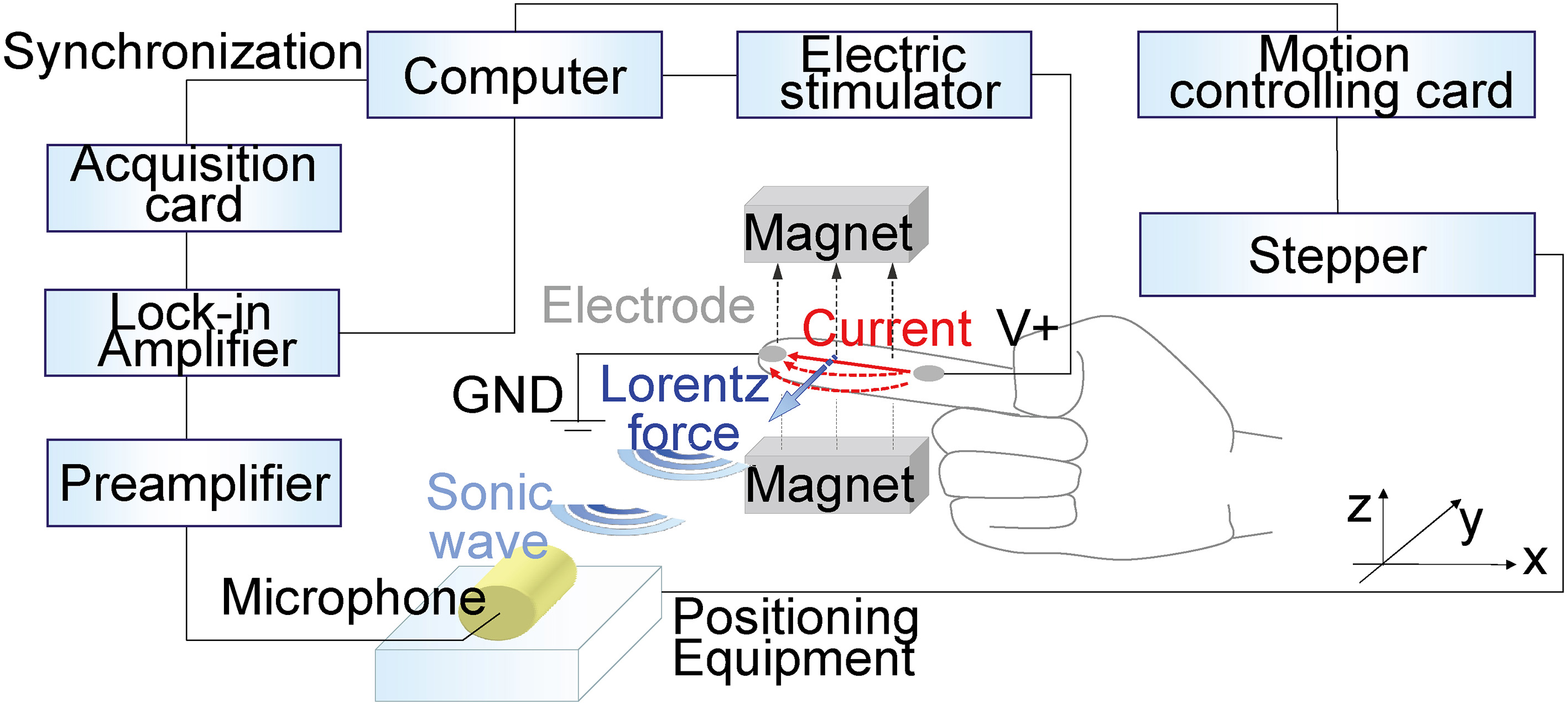
To obtain high detection and location accuracy, a magneto-acoustic (MA) imaging method has been proposed [15, 16, 17]. The method involves the application of a time-varying current to a sample in a static magnetic field. The current in the sample is influenced by the Lorentz force. Particles in the tissue vibrate and generate a sonic wave. The sonic signal is measured, and thus, the current distribution and the acoustic source can be located [18, 19], as shown in Fig. 1. The linear propagation of the sonic wave [20] avoids the current dispersion effect; therefore, a high-resolution measurement of the current can be achieved by locating the sonic source [21]. Bioelectrical current monitoring obtained valuable information from MA imaging. The approach is also beneficial for the early diagnosis of cancer [22] and other diseases related to the electrical properties of tissue.

Figure 1.

Scheme for detecting a MA wave using electric stimulating current.

Current studies are mainly based on short-pulse excitation, which involves a 100 V to 10 kV high-voltage pulse with a micro-second width for excitation [23, 24] to obtain a high MA signal level. However, due to the short duration of the pulse, the signal power is low. Moreover, the SNR and the detection accuracy are limited.

Methods of modified excitation have been developed. The step-in frequency and frequency-modulating method has been reported to increase the SNR [25]. However, the transducer needs to be band calibrated for multi-frequency measurements. The use of differential frequency ultrasound to generate a MA signal has been studied to increase the SNR, but the resolution is limited [26]. Coded excitation is used to improve the SNR of the MA signal [27]. The MA signal is then measured and compressed. Results indicate that this method provides a bigger SNR improvement and requires less time than waveform averaging method. However, the code length limits the SNR improvement.

The use of the lock-in amplification method [28] to improve the accuracy of MA signals in detecting bioelectric currents has been reported [29]. This approach improves the measuring accuracy, but only the amplitude of a single frequency amplitude is measured. Thus it is difficult to locate the sonic source using this method.

We have proposed a new approach for locating the MA source of sample conductivity in vitro by using lock-in measurements [30]. However, there are no reports on MA signal measurement or source location for in vivo human samples.

In this study, the measuring system is updated to achieve higher accuracy in locating the sonic source. An in vivo study on the human finger under electrical stimulation is performed, and the measurement and location accuracy of the sonic source are investigated.

2.Theory

The wave equation of MA effect in the frequency domain is [23]

wherein 𝑷⁢(𝒓,j⁢ω) is the MA signal in the frequency domain; 𝒓 is a space variable; 𝑱 is the current density; The Lorentz force density 𝑭=𝑱×B0; 𝑩0 is the flux density of magnetic field. S⁢(j⁢ω) is the electrical stimulation; H⁢(j⁢ω) is the imaging system function; ω is the angular frequency; and c is the sound transmitting speed in the medium.

Using the Green’s function in the frequency domain, the MA signal can be separated into temporal and spatial terms [31], and the sound signal in the frequency domain expression is

where 𝒓0 is the detection point. ∇⋅𝑭=∇⋅(𝑱×B0) is the acoustic source, and it can be observed that the sonic source contains the current distribution of the sample. ej⁢ω⁢|𝒓-𝒓0|/c is the transmitting delay caused by the detection distance, which is reflected in the phase. 1/(4⁢π⁢|𝒓0-𝒓|) is the transmission coefficient of the sound wave over a specified distance, which is reflected in the amplitude.

We have established a Cartesian coordinate system, as is shown in Fig. 1. The stimulating current is along the x direction. The magnetic field is along z direction. The sonic wave transmits along -y direction. Here we suppose the sample size is smaller than the measuring distance to the spherical sonic wave.

where 𝑱i=Ai⁢𝑱^, Ai is the amplitude, 𝑱^ is the unit current density of 𝑱; li is the distance from the i-th discrete sample pixels to the detector. The size of the summation pixels are x0⁢z0⁢Δ⁢l.

The sonic pressure from the i-th source is

If the stimulation is a sinusoidal signal, the spectrum components are all zero except for the excitation frequency. Therefore, the term -c⁢[∇⋅(𝑱^×𝑩0)]⁢(1/4⁢π)⁢x0⁢z0⁢Δ⁢l⁢S⁢(j⁢ω)⁢H⁢(j⁢ω) can be considered a constant.

The amplitude and phase of 𝑷i⁢(𝒓,j⁢ω) are

As is known, a single-frequency sinusoidal signal s⁢(t)=A1⁢sin⁡(ω⁢t+Φ1) from the sonic source can be represented as a vector (A1,Φ1)=(A1,j⁢ω⁢l1/c) in the complex plane, where l1 is measuring distance. The real part is A1⁢sin⁡Φ1, and the imaginary part is A1⁢cos⁡Φ1.

Figure 2.

Scheme of the vector summation of the sonic sources.

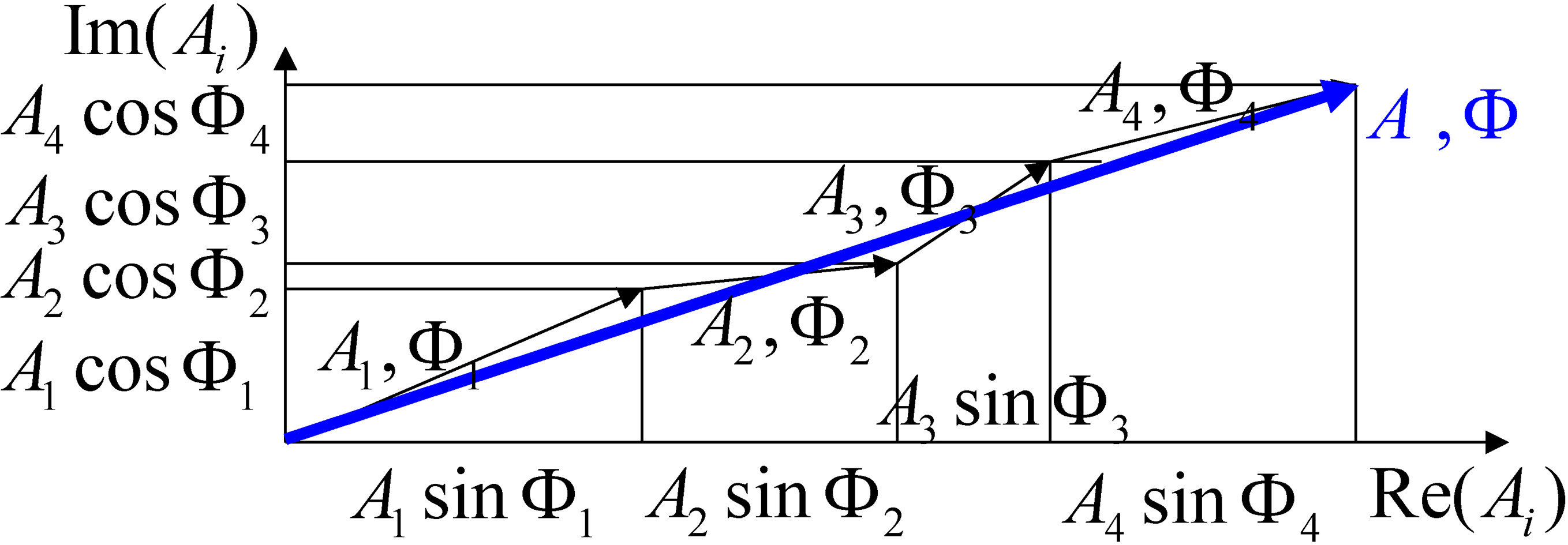
Suppose the sample is formed by n source points, MA signal is calculated by the vector summation, as shown in Fig. 2.

The amplitude A and phase Φ are

If the electrode distribution and the sample parameters are known, the stimulating current distribution in the sample can be calculated by the finite element method. Therefore, the amplitude A and phase Φ of each sonic source pixel can be calculated according to Eq. (7). In experiments, A and Φ can be measured by a lock-in amplifier.

Assuming the excitation signal period is T, the phase Φ can be expressed as follows:

This expression indicates that the measured phase is linearly related to the location of the sonic source.

3.Method

The structure of the experimental system is shown in Fig. 3. The function generator output is controlled by a computer, including the waveform, magnitude, phase, and frequency of the exciting signal. A power amplifier is used to strengthen the output power.

Figure 3.

Photographs of the experimental system. (a) Experimental system. (b) Plate with electrodes. (c) Sample measurement.

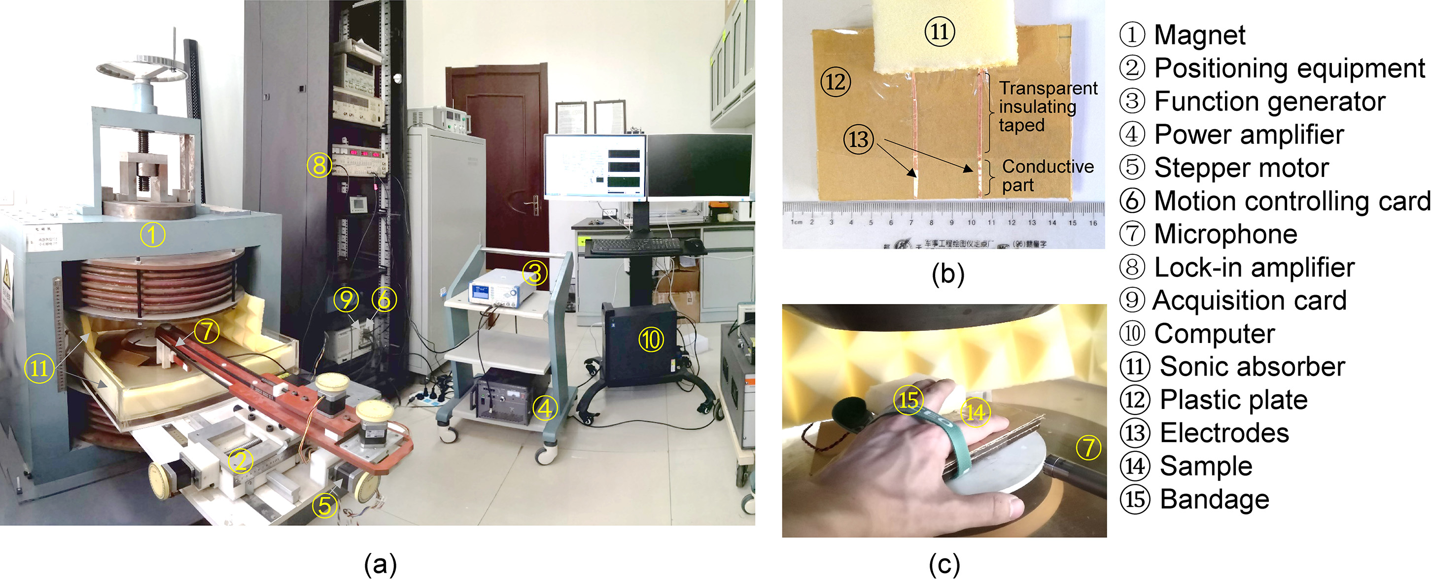
The sample is placed in a uniform static magnetic field. The cylindrical uniform magnetic field is 0.3 Tesla with 5 cm radius and 10 cm height. The flux density of the magnetic field. The nonuniformity of flux density is less than 6%. Meanwhile, the function generator outputs a synchronous signal, which is connected to the lock-in amplifier as a reference signal.

The motion controlling card (PXI7340, NI, USA) is used for motion control, including the output of the controlling code, to enable the motor to step in. The minimum step angle of the stepper motor (NEMA 23, Danaher, USA) is 1.8∘.

Space-positioning equipment is used to drive the microphone to move over 5 degrees of freedom: along the x, y, and z axes, sensor rotation and sample rotation. The x axis screw pitch is 3 mm, the y axis screw pitch is 4 mm, and the z axle screw pitch is 3 mm. In this study, only y axis direction (along the normal of the microphone detection surface) is used.

The microphone converts the MA signal to a voltage signal. The microphone is a polarized microphone (4955, B&K, Denmark) whose frequency response is 5 Hz to 20 kHz. The gain can be set by adjusting the preamplifier module (2690, B&K, Denmark). The sensitivity of the microphone is set to 100 V/Pa.

The MA signal is measured by the lock-in amplifier (LI5640, NF, Japan) according to reference signals from the function generator. The measured signal is eventually adopted by an acquisition card (PXI5922, NI, USA) and then processed and stored.

The electrode is made of a strip copper foil and adhered to a plastic plate. The conductive part of the copper foil measures 2 cm and is placed in contact with the sample. The other parts are sealed with transparent insulating tape to avoid accidental contact. The hand is tied by a bandage to avoid movement. The sample and the plastic plate are adhered in the magnetic field. The sonic absorber sponge is set to reduce noise. Pyramid-shaped sponges are also set around the sample and the microphone.

4.Results

We aimed to preliminarily validate the method of locating MA sources. The detection accuracy of the amplitude and phase of the MA signal using lock-in measurements is investigated. A human finger is used as an in vivo experimental sample.

4.1Experimental results under different excitation levels

A human finger (in vivo) is used to test the measurement accuracy. The finger is fixed in the magnetic field. The exciting frequency is 10 kHz. The resistance of the finger is 5.04 ± 0.72 kΩ, as measured by an LCR tester (3522–50, Hioki, Japan) ten times. The resistant measurement positions are the same as the planned contact positions of the stimulating electrodes. The two contact points are located on the first and third joints on the front of the index finger. Conductive paste is applied to the contact points. In a preliminary study, the conductivity of the finger sample is considered uniform and taken as the entire sonic source. The gap between the two electrodes is 3 cm. The detection distance is 7 cm. The measured amplitudes and phases under various excitation currents are shown in Fig. 4a.

Figure 4.

Amplitude and phase of MA signal under various levels of excitation (sinusoidal wave). (a) Results for various exciting amplitudes. (b) Results for various exciting phases.

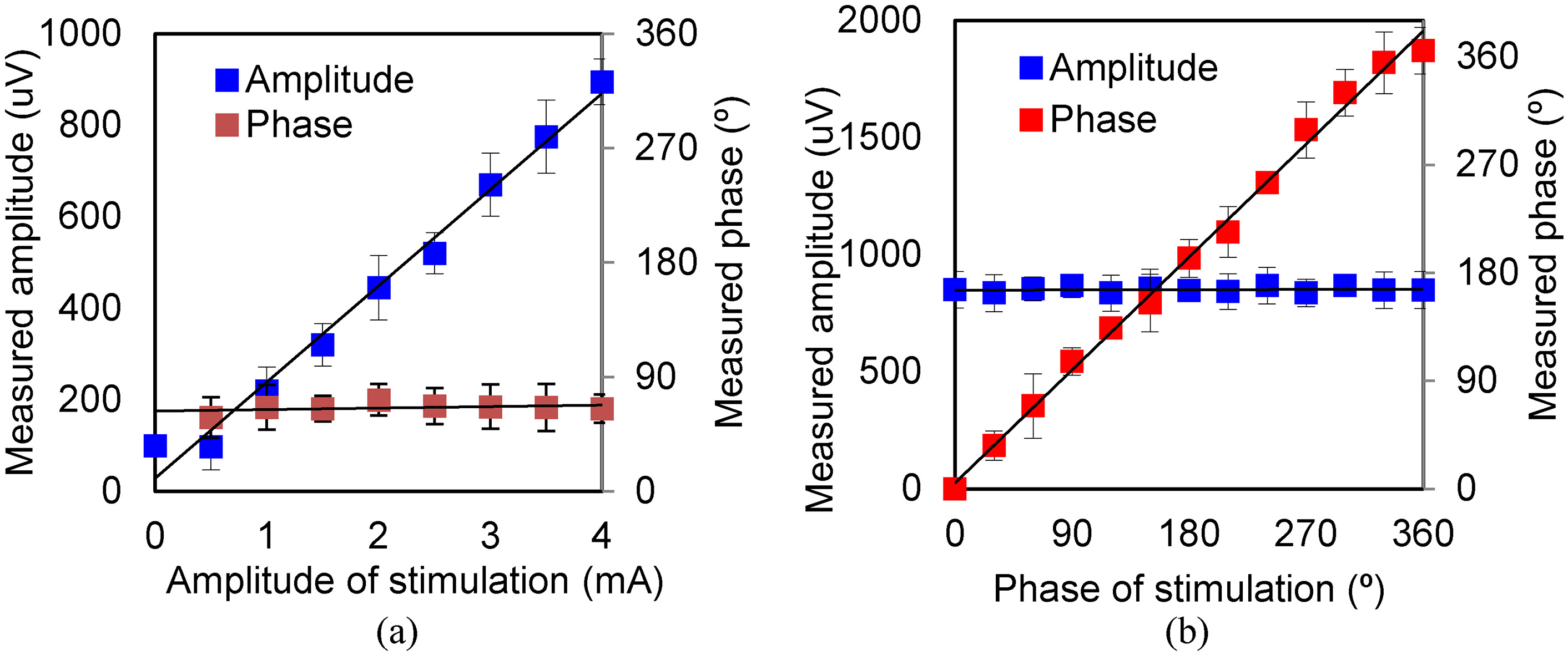
As shown in Fig. 4a, when the excitation current varies from 0.5 mA to 4 mA, the measured amplitude of the MA signal varies linearly, whereas the phase is a constant, indicating that the sonic source can be located from the phase. After calculation, the detection accuracy of the MA signal is 10-6–10-7 Pascal.

The parameters measured under an excitation current of less than 0.5 mA are affected by noise. The results show, the MA signal is extracted under 0.5 mA excitation, at the same time, the sonic source is located.

The amplitudes and phases measured under various excitation phases are shown in Fig. 4b. The excitation phase is set from 0∘ to 360∘. The exciting amplitude is 4 mA. The exciting frequency is 10 kHz, and the detecting distance is 7 cm.

We measure the MA signal amplitude and phase. Figure 4b shows that the measured MA signal phase increases linearly with the phase of the excitation, while the amplitude remains unchanged.

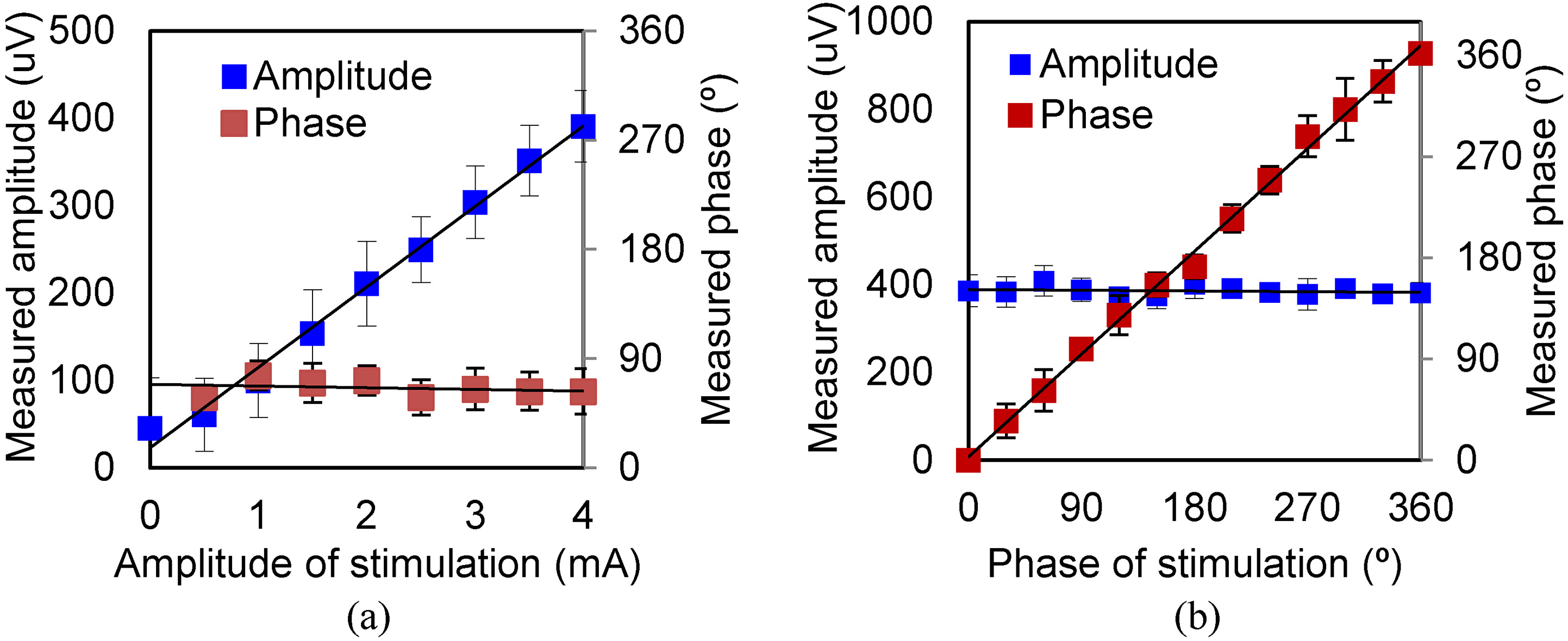
The amplitudes and phases under triangular wave and square wave excitation with the same amplitude and frequency are also measured and are shown in Figs 5 and 6. The curves show similar characteristics. The amplitudes of the triangular and square waves are smaller than those of the sinusoidal wave. The reason is that, at the same repetition frequency, the spectral range of the square wave and triangular wave is wider than that of the sinusoidal wave, and the spectral composition at 10 kHz is lower.

Figure 5.

Amplitude and phase of MA signal under various levels of excitation (triangular wave). (a) Results for various exciting amplitudes. (b) Results for various exciting phases.

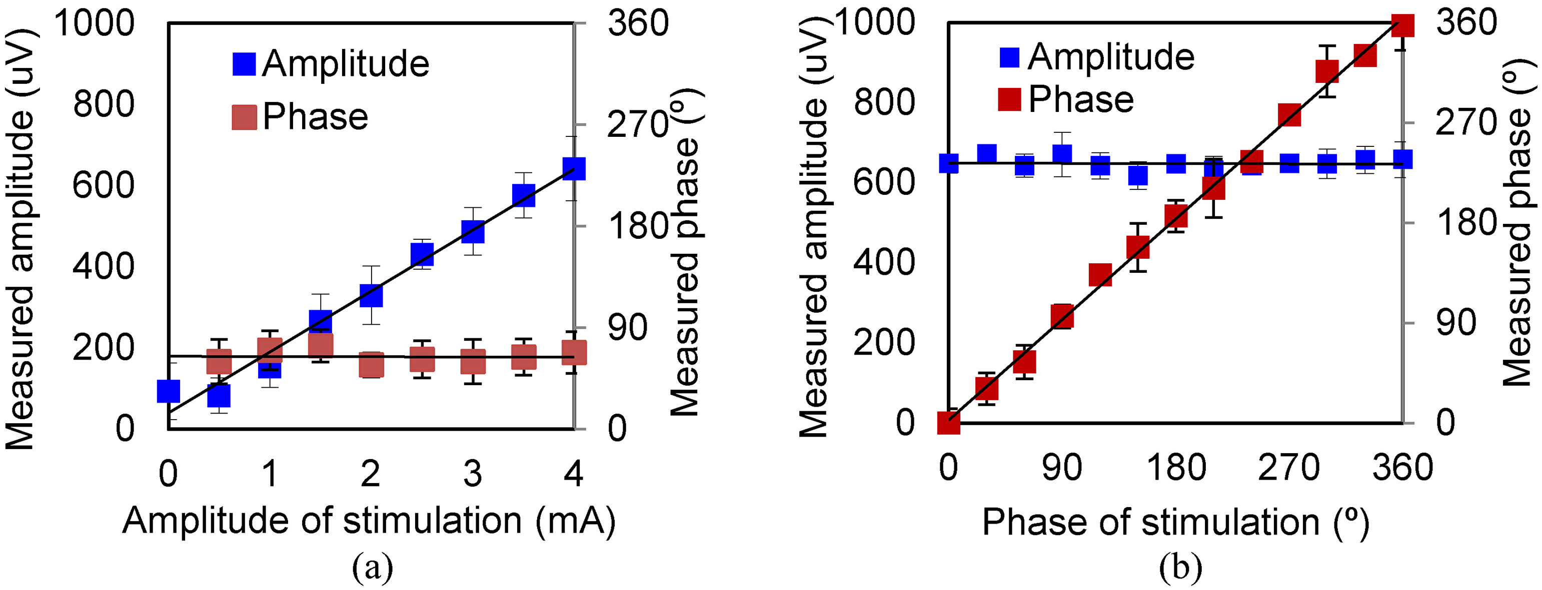
Figure 6.

Amplitude and phase of MA signal under various levels of excitation (square wave). (a) Results for various exciting amplitudes. (b) Results for various exciting phases.

The result of the experiment under various excitation levels illustrates that the designed measurement system can detect signals from an in vivo human finger sample under the mA excitation. The measurement accuracy is improved to less than 1 μPa, and the sonic source can be located.

4.2Experimental results obtained at different detection distances

To investigate the locating characteristics of the sonic source of the proposed system, the amplitude and phase curves with distances are measured.

The excitation is 4 mA with 5 k, 10 k and 20 kHz frequencies. Because the nickel shell of the microphone is influenced by the magnetization effect over an area with a radius less than 50 mm, the detection distance is set to 50, 55, … 125 mm. The measured and simulated (according to Eq. (7)) amplitude and phase curves are shown in Fig. 7. The simulating parameters are same as reference [30]. In the experiment, we treat the finger as the entire sonic source; therefore, in the corresponding simulation, we also treat the finger as the entire source.

Figure 7.

Measured amplitude and phase at different distances.

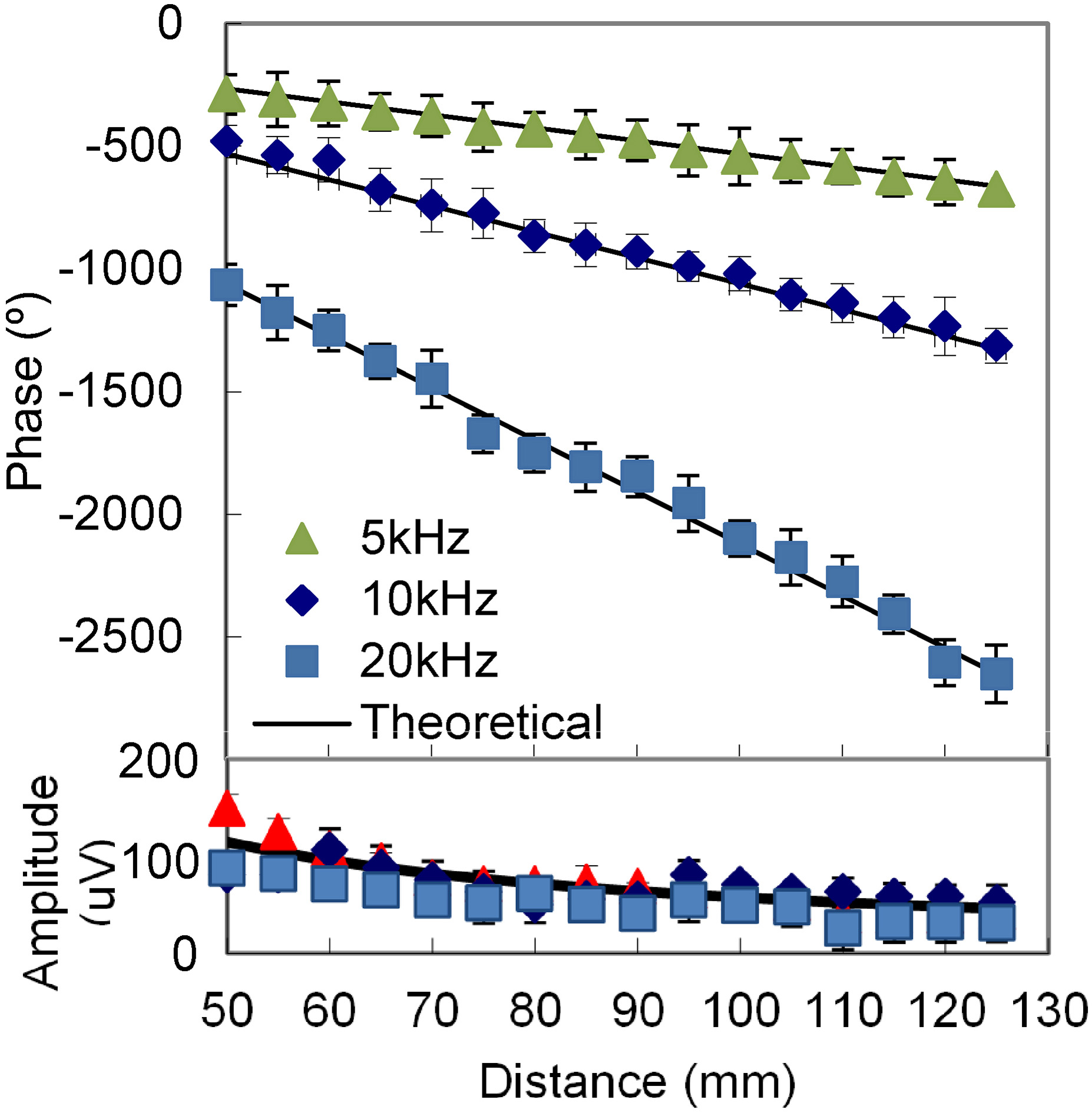
As shown in Fig. 7, the measured amplitudes decrease when the distance increases. The relative errors between the measured and theoretical data at the three frequencies are 12.2%, 18.5%, and 22.6%. The results show that the errors of amplitude at high frequency are larger than at low frequency. The reason is the acoustic wave attenuation at high frequency is greater than that at low frequency. The background noise affects the measurement at high frequencies much more than low frequencies. In addition, the environment and circuit noise cause deviation. This deviation can be suppressed by improving the noise shield equipment and filtering. Over the range of 60–125 mm, the phases change are 22.3∘, 52.8∘, and 97.5∘ every 5 millimeters at the three frequencies, which agree with the simulations. The errors between the measured and the theoretical phases are 10.9∘, 25.6∘, and 31.9∘, respectively. The errors is due to the movement error of the locating equipment. Environmental noise disturbance may be another reason.

Figure 8.

Measured phase at different distances. (a) 10 kHz square wave excitation. (b) 10 kHz triangular wave excitation.

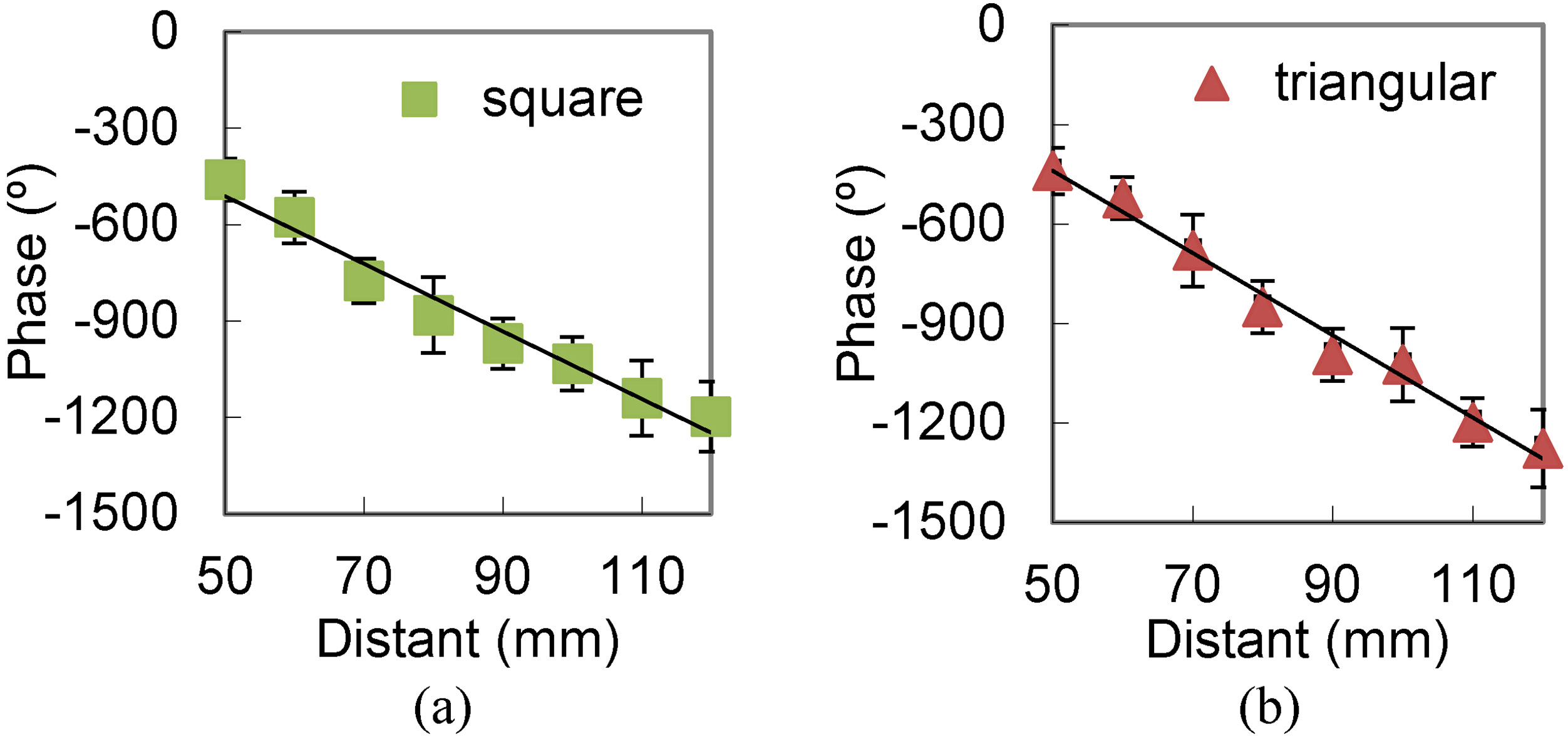
Figure 8 shows the phase characteristics under 10 kHz triangular and square waves. The figure shows similar results for the two waves. The results indicate the location characteristics of the sonic source of the phase in frequency.

4.4Location accuracy analysis of frequency domain imaging system

Based on the previous experiment, the phase of the MA signal reflects the position of the sonic source. To test the proposed method’s performance in locating the sonic source, the phase characteristics at various positions of the sample are examined.

We set the initial detection distance to 0.1 m. Then, we drive the positioning module to move a certain distance: 0.1 mm, 1 mm, or 10 mm. The phase changes of the MA signal are recorded to produce 512 experimental results. The average phase changes and standard deviations of the 512 statistical data are calculated. The results are shown in Table 1.

Table 1

Phase measurement accuracy results

Moving distance	5 kHz		10 kHz		20 kHz
(mm)	Phase (∘)	Standard deviation	Phase (∘)	Standard deviation	Phase (∘)	Standard deviation
0.01	-0.70	0.67	-5.55	5.78	0.26	1.96
0.1	-2.69	0.39	-0.38	3.19	-0.58	5.63
1	-0.76	1.21	-17.4	1.83	-15.33	3.70
10	-23.70	1.17	-73.6	1.97	-154.05	3.82

Figure 9.

Measured phase under 10 kHz sinuous wave at different electrode distances.

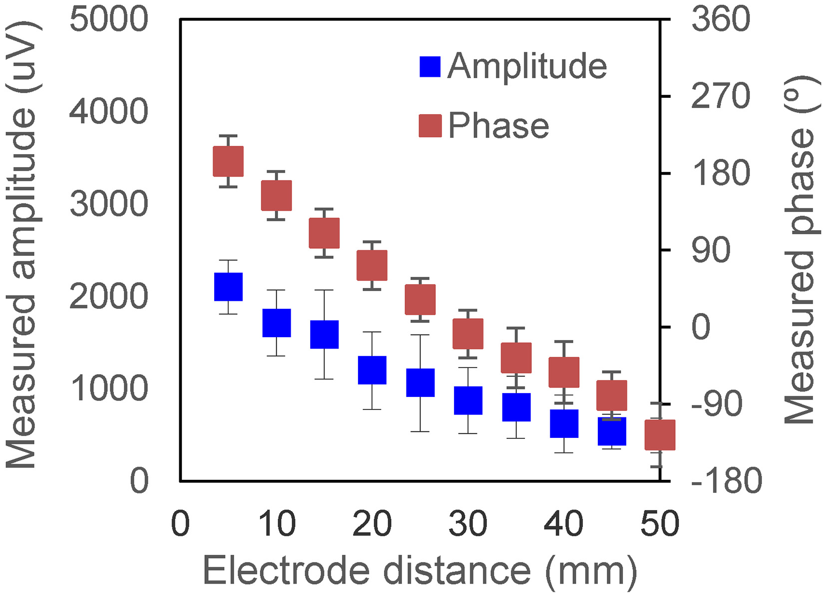
Table 1 shows that at 0.01 mm and 0.1 mm distance, the standard deviation of the phase change is greater than the average value of the signal phase, and the phase cannot be estimated, which means that the sonic source cannot be located by the MA signal. For a distance change greater than 1 mm, the standard deviation of the signal phase is less than the average value, and the phase can be estimated. The results show that the designed equipment allows for millimeter-level accuracy in locating the MA source.

5.Discussion

A method for locating a MA sonic source under electrical stimulation is examined in this study. The amplitude measurement accuracy of the MA signal and the phase locating accuracy are tested. Experimental results show that the amplitude accuracy of the imaging system is less than 1 μPa. The location accuracy is on the scale of millimeters. Several points should be noted.

First, in this article, a human finger is regarded as an integrated sound source in preliminary studies. And a microphone is used to detect the sonic signal. For measuring the internal structure of the sample, we need to separate the sample into several elaborate parts. Thus, the amplitude and phase of a single frequency are not enough for sonic sources reconstructing and locating. We need to design multi-microphones or multi-frequency measurement strategy to locate the sound sources. In MA imaging, the sound source locates at the position where the conductivity changes. Considering the propagation of MA signals. The MA signal measured by the microphone is the summation of several sound sources along the axis of the microphone. So if we image the sonic source inside the medium and the current distribution, we need to determine the intensity and location of all sound sources along this propagating path. However, only two parameters, the amplitude and the phase, can be measured by the lock-in amplifier when using a single-frequency sinusoidal wave stimulation. It is obviously insufficient for image reconstruction. In order to obtain more data, we consider that, the excitation frequency can be changed to f+Δ⁢f, f+2⁢Δ⁢f, etc. Δ⁢f is far less than stimulating frequency f, so it will have little impact on the stimulus effect to the body. (For example, the exciting frequency is changed from 10 kHz to 10.01 kHz, 10.02 kHz.) Thus, we can get more amplitudes and phases including the distribution of sound sources. According to Eq. (5), an equations can be set to calculate the intensity and location of MA sources, and reconstruct the image. Of course, the finger is regarded as the entire sound source in this study, which is an approximation. We preliminarily verify feasibility of measuring the MA signal magnitude and phase by lock-in amplification to in vivo samples. It provides an important basis for the follow-up imaging study of complex sample in vivo. At the same time, measurement data gathered from different samples must be processed. One possible solution is to obtain the inner tissue boundary distribution of each sample according to its structure image, such as an ultrasonic echo image. That image can be used as the benchmark data of the sample. Then, the functional information of the current distribution can be obtained through the MA imaging measurement method based on the benchmark data.

Second, the results show that under an excitation less than 0.5 mA, noise will affect the signal measured by the experimental equipment. It can be estimated that the noise magnitude is acceptable in the preliminary experiments because the electrical stimulation magnitude is typically greater than 10–100 mA. Noise will affect the experimental results when the MA signal is small, and subsequent experiments can reduce the effect of noise by redesigning a more closely measuring device. Additionally, a fibre optic hydrophone or laser vibrometer may be adopted to eliminate electromagnetic noise.

Third, different impedances due to skin moisture affect the measurement results. When the skin is wet, the salt in the sweat on the skin’s surface will lead to a decrease in contact impedance. The current will enter the tissue more easily under the same excitation voltage, thus forming a larger current in the tissue, and the MA signal will be larger than that on dry skin. Therefore, the MA signal will be easier to detect, and the signal-to-noise ratio (SNR) will be higher under the same level of background noise. Furthermore, a higher sonic source location accuracy will be attained. However, sweat on the skin’s surface may form a current circuit. Part of the current would flow only through the surface, not enter the tissue, and form MA signals, which would influence the measurement. Therefore, this effect must be evaluated in subsequent studies.

Fourth, changes in sample shape during an experiment will affect the measurement. For in vivo experiments in particular, shape changes are inevitable, causing changes in the measurement data, as indicated in Eqs (5) and (7). Movement can be reduced by fixing the sample with specialized equipment. Moreover, by upgrading the hardware used for multi-channel detection, lock-in measurement and high-speed acquisition, position movement can be captured in real time, thus reducing the error caused by movement.

In addition, when the phase change is greater than 360 degrees, the lock-in amplitude cannot distinguish the difference between Φ and Φ+ 360∘; thus, the imaging range presents a problem. The imaging range is approximately 15 centimeters in the soft tissue under the excitation of 10 kHz. which is sufficient for general electrical stimulation to image the stimulating current. If a larger imaging range is required, a lower excitation frequency, such as 5 kHz (imaging range = 300 mm), can be used. However, higher noise levels in tissue should be suppressed in the measurement.

Furthermore, when measuring the acoustic signals near the sample, the acoustic wave is plane wave, which is not accord with the 1/l trend according to the Eq. (1). Therefore, a strict mathematical model, which is close to the real biological tissue samples, should be studied to validate the test results in future studies.

In conclusion, a method for locating a MA source using lock-in measurement will be valuable for current distribution imaging under electrical stimulation and thus will be beneficial for optimizing the parameters of electrical stimulation, improving the targeting of electrical stimulation, and improving the effect of stimulation therapy for neuropathy. This method will also be valuable for studying the activity of neurons, further revealing the powerful ability of electrical stimulation to regulate nerve excitability and playing an active role in research on tissue rehabilitation and neural regulation and control.

References

[1] | Peckham PH, Knutson JS. Functional electrical stimulation for neuromuscular applications. Annual Review of Biomedical Engineering. (2005) ; 7: (7): 327. |
[2] | Hiroyuki M, Abbas O, Hitoshi O, Genichi T, Kotaro T, Shigeru S. Ability of electrical stimulation therapy to improve the effectiveness of robotic training for paretic upper limbs in patients with stroke. Medical Engineering & Physics. (2016) ; 38: : 1172-1175. |
[3] | Nakipoğlu GF, Köse DB, Özgirgin N. A randomized controlled study: effectiveness of functional electrical stimulation on wrist and finger flexor spasticity in hemiplegia. Journal of Stroke and Cerebrovascular Diseases. (2017) ; 26: : 7. |
[4] | Tsuchiya M, Morita A, Hara Y. Effect of dual therapy with botulinum toxin an injection and electromyography-controlled functional electrical stimulation on active function in the spastic paretic hand. Journal of Nippon Medical School. (2016) ; 83: (1): 15-23. |
[5] | James AH, Robert AG, Douglas JW. Effects of Synchronous Electrode Pulses on Neural Recruitment during Multichannel Microstimulation. Scientific Reports. (2018) ; 8: : 13067. |
[6] | Moe JH, Post HW. Functional electrical stimulation for ambulation in hemiplegia. The Journal-Lancet. (1962) ; 82: : 285-288. |
[7] | Luca M, Roberto M. Distribution of electrical stimulation current in a planar multi layer anisotropic tissue. IEEE Transactions on Biomedical Engineering. (2008) ; 55: : 660-670. |
[8] | Gabriel C, Gabriely S, Corthout E. The dielectric properties of biological tissues: II. Measurements in the frequency range 10 Hz to 20 GHz. Physics In Medicine and Biology. (1996) ; 41: : 2231-2249. |
[9] | Margaret C, David I, Jonathan CN. Electrical impedance tomography. IEEE Signal Processing Magazine. (2011) ; 18: (1): 35-41. |
[10] | Yang L, Can-Hua X, Shi X, Feng F, Dai M, Xia J, Jing L, Xiuzhen D. Calibration method based on multi-frequency electrical impedance tomography system. Chinese Medical Equipment Journal. (2014) ; 10: (2): 355-366. |
[11] | Joy M, Scott G, Henkelman M. In vivo detection of applied electric currents by magnetic resonance imaging. Journal of Magnetic Resonance Imaging. (1989) ; 7: (1): 89. |
[12] | Jin KS, Yoon JR, Woo EJ, Kwon O. Reconstruction of conductivity and current density images using only one component of magnetic field measurements. IEEE Transactions on Biomedical Engineering. (2003) ; 50: (9): 1121-1124. |
[13] | Dallas WJ, Smith WE, Schlitt HA, Kullman W, Dwyer SJ, Schneider RH. Bioelectric current image reconstruction from measurement of the generated magnetic fields. Proc SPIE Medical Imaging. (1987) ; 767: : 2-10. |
[14] | Oyama D, Higuchi M, Adachi Y, Kawai J, Uehara G, Hisashi KH, Kobayashi K. Electric current imaging by ultrasonography and SQUID magnetometry. IEEE Transactions on Applied Superconductivity. (2011) ; 21: (3): 440-443. |
[15] | Roth BJ, Basser PJ, Wikswo JP. A theoretical model for magneto-acoustic imaging of bioelectric currents. IEEE Transactions on Biomedical Engineering. (1994) ; 41: (8): 723-728. |
[16] | Wen H. Volumetric Hall Effect tomography-a feasibility study. Ultrasonic Imaging. (1999) ; 21: (3): 186-200. |
[17] | Bruce CT, Mohammed RI. A Magneto- Acoustic Method for the Noninvasive Measurement of Bioelectric Currents. IEEE Transactions on Biomedical Engineering. (1988) ; 35: (10): 892-894. |
[18] | Hu G, He B. Magnetoacoustic imaging of magnetic iron oxide nanoparticles embedded in biological tissues with microsecond magnetic stimulation. Applied Physics Letters. (2012) ; 100: (1): 13704. |
[19] | Zhang S, Ma R, Yin T, Liu Z. Research on the time-frequency characteristics of the magneto-acoustic signal in media of different thicknesses based on the wave summing method. Journal of Medical Imaging and Health Informatics. (2017) ; 7: (2): 453-459. |
[20] | Fei C, Chiu CT, Chen X, Chen Z, Ma J, Zhu B, Shung KK, Zhou Q. Ultrahigh frequency (100 MHz–300 MHz) ultrasonic transducers for optical resolution medical imagining. Scientific Reports. (2016) ; 6: : 28360. |
[21] | Emerson JF, Chang DB, Mcnaughton S, Jeong JS, Shung KK, Cerwin SA. Electromagnetic acoustic imaging. IEEE Transactions on Ultrasonics Ferroelectrics. (2013) ; 60: (2): 364-372. |
[22] | Salim MI, Supriyanto E, Haueisen J, Ariffin I, Ahmad AH, Rosidi B. Measurement of bioelectric and acoustic profile of breast tissue using hybrid magnetoacoustic method for cancer detection. Med Bio Eng Comp. (2013) ; 51: (4): 459. |
[23] | Mariappan L, Hu G, He B. Magnetoacoustic tomography with magnetic induction for high-resolution bioimepedance imaging through vector source reconstruction under the static field of mri magnet. Medical Physics. (2014) ; 41: (2): 022902. |
[24] | Hu G, He B. Magnetoacoustic imaging of electrical conductivity of biological tissues at a spatial resolution better than 2 mm. Plos One. (2011) ; 6: (8): e23421. |
[25] | Aliroteh MS, Scott G, Arbabian A. Frequency-modulated magneto-acoustic detection and imaging. Electronics Letters. (2014) ; 50: (11): 790-792. |
[26] | Renzhiglova E, Ivantsiv V, Xu Y. Difference frequency magneto-acousto-electrical tomography (DF-MAET): application of ultrasound-induced radiation force to imaging electrical current density. IEEE Transactions on Ultrasonics Ferroelectrics and Frequency Control, (2010) ; 57: (11): 2391-2402. |
[27] | Zhang S, Zhou X, Liu S, Yin T, Liu Z. Research on barker coded excitation method for magneto-acoustic imaging. Biomedical Signal Processing and Control. (2018) ; 39: : 169-176. |
[28] | Meade ML. Lock-in amplifiers: Principles and applications. Majalah Lapan. (1983) ; 131: (3): 134. |
[29] | Roth BJ. The role of magnetic forces in biology and medicine. Advances in Experimental Medicine and Biology. (2011) ; 236: (2): 132. |
[30] | Zhang S, Zhou X, Yin T, Liu Z. Magneto-acoustic imaging by continuous-wave excitation. Medical & Biological Engineering & Computing. (2017) ; 55: (4): 595-607. |
[31] | Xu Y, He B. Magnetoacoustic tomography with magnetic induction (MAT-MI). IEEE Transactions on Medical Imaging. (2010) ; 29: (10): 1759-1767. |