Applied current thermoacoustic imaging for biological tissues

1.Introduction

In the past decades, more and more attention has been paid to the imaging method based on thermoacoustic effect [1, 2, 3, 4]. In the thermoacoustic effect, a biological tissue is irradiated in an electromagnetic field. The tissue absorbs some electromagnetic energy, and then because of thermo elastic expansion it subsequently leads to ultrasonic wave emission. The acoustic waves are related to the properties of the tissue, and could be collected by the ultrasound transducers setting around the tissue [5, 6]. Photoacoustic imaging [7, 8] and microwave-induced thermoacoustic imaging [9, 10] are two imaging modalities based on the thermoacoustic effect. Photoacoustic imaging, which uses light as excitation source, is only suitable for superficial applications. Compared with photoacoustic imaging, microwave-induced thermoacoustic imaging, which uses microwave radiation, obtains deeper penetration. The imaging depth depends on the tissue properties and the electromagnetic frequency used for irradiation. In principle, using lower frequencies can achieve deeper penetration [11].

To explore a potential imaging method for deeper penetration, Zheng et al. have theoretically studied the feasibility using radio frequency magnetic field below 20 MHz to electric conductance or magnetic nanoparticles targets to modulate thermoacoustic imaging, called magnetically mediated thermoacoustic imaging (MMTAI) [12, 13]. A metal sample was used to experiment with, and the theromacoustic imaging was obtained, which was similar to the sample in terms of shape, and a coherent frequency domain method was discussed in great detail. The imaging method has broad prospects for the development of thermoacoustic imaging using low frequency magnetic field, and it has been preliminarily proved by the results of numerical simulation and physical experiment. In this paper, we report a new imaging method called Applied Current Thermoacoustic Imaging (ACTAI). In ACTAI, a μs width pulse current is injected into the biological tissue. The biological tissue absorbs the Joule heating, thereby destroying the thermodynamic equilibrium inside it and then the tissue expends and emits ultrasonic waves. The thermoacoustic waves can reflect the conductivity distribution. Meanwhile, the large differences of electrical characteristics can be used to reflect the physiological and pathological changes about biological tissues, and it can provide evidence for the early diagnosis and treatment of cancer in potential applications [14, 15, 16, 17]. In this paper, one thermoacoustic image of a piece of pork was obtained for the first time, which reflects the conductivity change of the pork well. Compared to ACTAI, MMTAI needs high-power excitation to generate an alternating electromagnetic field inducing current inside the tissue. In contrast, ACTAI only needs a small safe current passing through the tissue. Therefore the equipment of ACTAI is simpler and more convenient for deeper penetration. In this paper, for the first time the principles of ACTAI are presented. The simulation in a sample is demonstrated, in which the acoustic signals and a B-scan image are shown. The experimental method and setup are presented in the experiments section, and the ACTAI signals and an image from pork are also given.

2.Theory

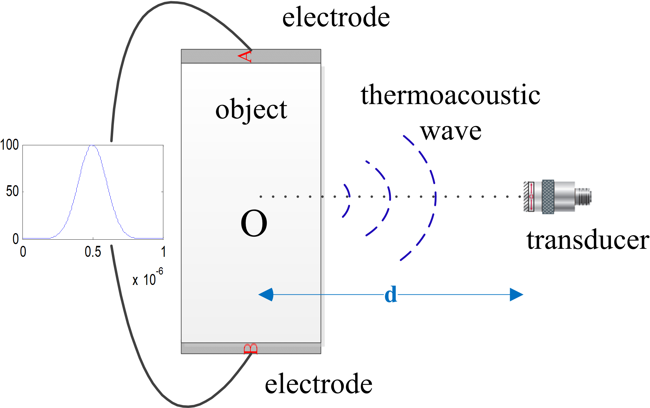
A theoretical analysis shows that the acoustic pressure has a relationship with the conductivity of the target, which is described by a detailed deduction. The conceptual framework of ACTAI is shown in Fig. 1. In ACTAI, the target is injected in a Gauss pulse current. This produces one pulse electric field 𝑬⁢(r′,t) inside the target, where r′ is the location in it. The regions of A and B are the injection electrodes. The electric potential of A is U⁢(t) and the potential of B is 0. The injection current pulse used in ACTAI is an approximate microsecond level current. The target is an isotropic and homogeneous medium and its conductivity distribution is σ⁢(r′). Both the target and transducer are covered with the transformer insulation oil, and the conductivity of insulation oil is zero. Under the quasi-static field, the governing equations for the boundary condition that the target satisfies could be described as follows:

Figure 1.

The principle of ACTAI.

where Γ and ϕ denotes an outer boundary of the target and an electric scalar potential of the target, respectively. According to Eq. (1), the ϕ can be obtained. The electric field of the target could be represented as 𝑬⁢(r′,t)=-∇⁡ϕ, on the basis of the Helmholtz Theorem. Thus the current density in the target is 𝑱⁢(r′,t)=σ⁢𝑬⁢(r′,t), which leads to the absorption of Joule heating. The heating function is defined as the energy absorbed per unit volume of time, denoted by Q⁢(r′,t). Its expression is:

where Q⁢(r′) is the spatial absorption function and I⁢(t) is the time description function [18, 19, 20, 21]. The spatial absorption function [22] is defined as Q⁢(r′)=𝑱⁢(r′)⋅𝑬⁢(r′)=σ⁢|E⁢(r′)|2, in which E⁢(r′) is the electric field at the position of r′. After absorbing Joule heating, the target emits thermoacoustic waves because of instantaneous expansion. The generation and propagation of the thermoacoustic signal for ACTAI is described by the general thermoacoustic wave equation:

where cs denotes the acoustic velocity, CP denotes the specific heat capacity, β denotes the isobaric volume expansion coefficient, and p⁢(r,t) is the sound pressure of time of t and in the position of r. In Eq. (3), the acoustic wave propagation is described in the left side, whereas the acoustic source term is the term of the right side. The acoustic signals can be received by ultrasonic transducers located around the target to image.

The sound pressure p⁢(r,t) in the position of r could be obtained by Green’s function [23, 24, 25, 26, 27], which is:

where Ω is the whole integration area including the all sound sources, r is the transducer position, and 𝒓′ the sound source position. By the electric field near and in the target, Eq. (4) is the basic formula to work out the sound pressure. The simulated or experimental signal is then used to reconstruct the spatial absorption function distribution Q⁢(r′) as described in the next section.

3.Numerical simulation

In order to verify the theory of ACTAI, the coupling analysis of electromagnetic field and acoustic field for low conductivity simulation model was carried out using the finite element method. In order to simulate tumor tissue surrounded by healthy tissues, the simulation sample was made by putting a square tumor tissue with 1 cm length into a rectangle healthy tissue with a size of 30 mm × 40 mm. The conductivity of the square tumor tissue and rectangle healthy tissues are set to 5 S/m and 1 S/m, respectively, which is shown in Fig. 2a. Coupling acoustic waves, using transformer insulation oil immerse the simulation model and the transducer, and the conductivity of the oil is 0 S/m. The velocity of sound wave of the transformer insulation oil was measured to be 1400 m/s, so the sound velocity is prescribed as 1400 m/s in the simulation. In the simulation of the sound field, it is assumed that the acoustic properties of the model and the oil are uniform, and the acoustic waves are not scattered, reflected and attenuated during the propagation. The expression of the voltage applied to the target is set to be V⁢(t)=100⁢e-(t-b)2/2⁢c2, in which b=5×10-7 and c=1×10-7, whose waveform is shown in Fig. 1. The center frequency of the transducer is 1 MHz. The gap space between the center of the target and the sound transducer is 2 cm, meaning the location of the sound detector is (20, 0) mm.

Figure 2.

The results of the simulation in the ACTAI. (a) The conductivity distribution in the target. (b) Normalized waveforms obtained by its detector.

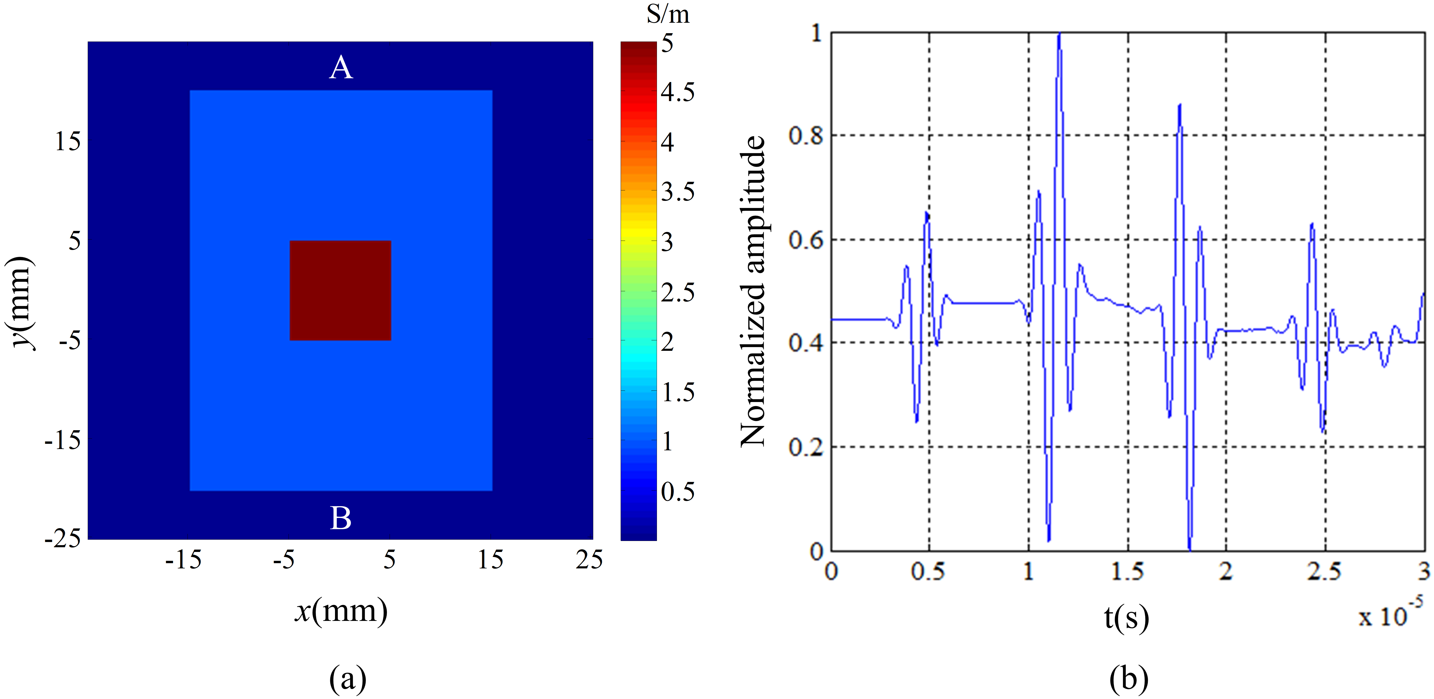
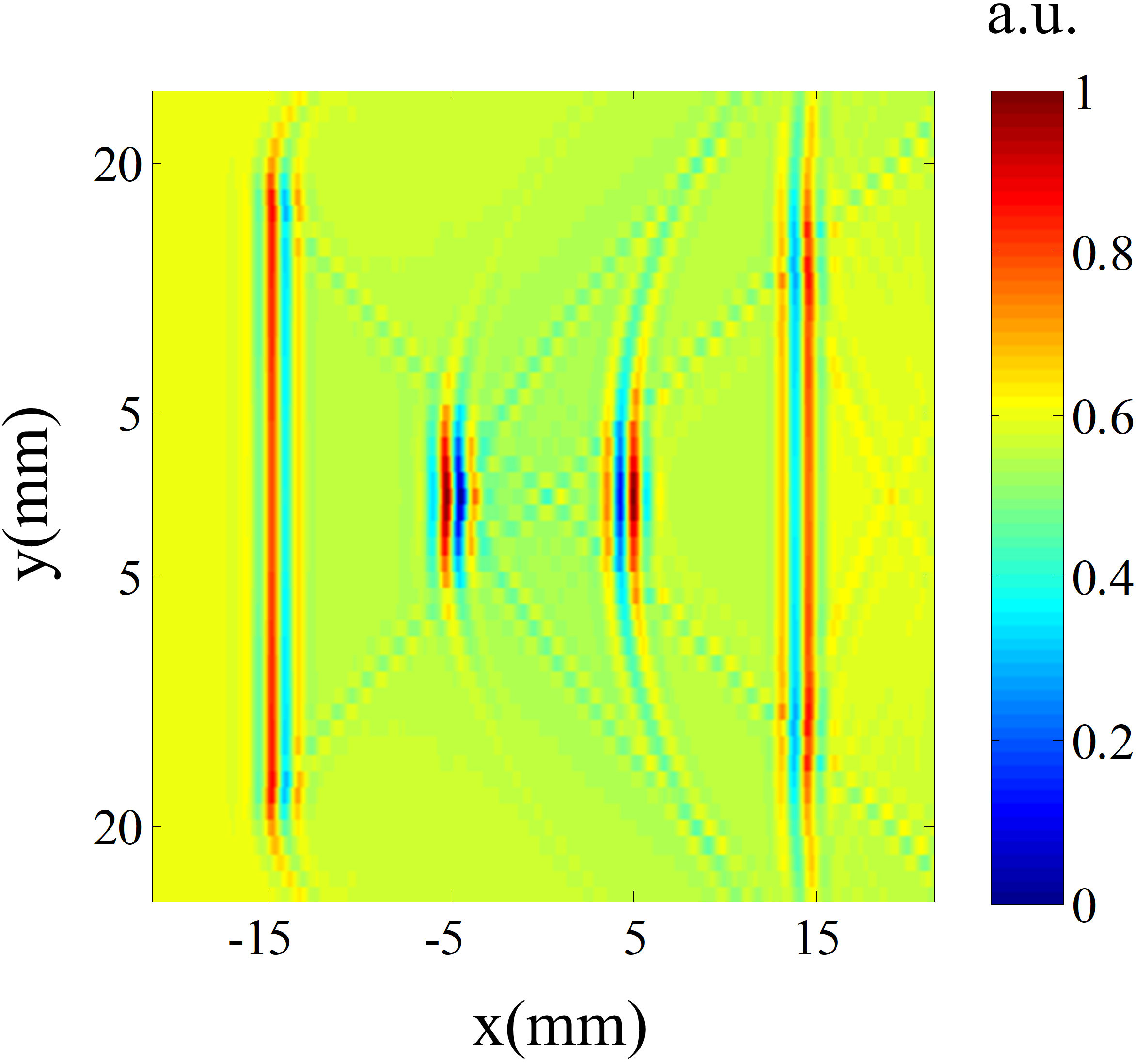
Figure 3.

B-scan image of the simulation model.

The signals received by the detectors are the convolution of the sound pressure and the impulse response of the sound transducers in practical experiments. So the simulation signals are processed with the convolution of the pressure to agree with the experiments. The normalized waveform detected by the transducer is obtained by Eq. (4) and shown in Fig. 2b. 3.5 μs is the appearance time of the wave clusters and 25 μs is the ending time of the wave clusters. It conforms to the propagation time of the sound waves from the two peripheral edges of the healthy simulation target to the ultrasonic detector. The second wave cluster is about at 10.7 μs, which coincides with the time of the sound wave propagation, and this time corresponds to the healthy-breast boundary to its transducer. The third cluster is about at 17.8 μs which coincides with the time of the sound wave propagation, and this time corresponds to the breast-healthy boundary to its detector. It proves that the sound pressure is generated by the simulation target, and it can also reflect the conductivity changes information of the target.

The transducer is moved in the line x= 20 mm of y direction from -24 mm to 24 mm in the step of 1 mm to acquire data. The B-scan image of this model was produced from the acoustic signals as shown in Fig. 3, which shows the target structure. It displays the boundary changes of the conductivity.

Figure 4.

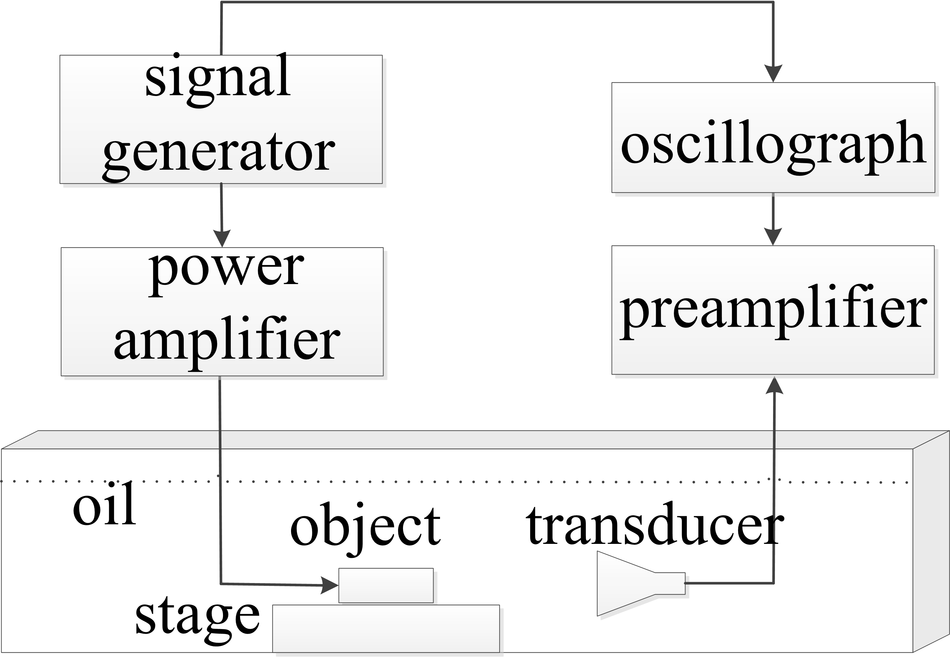
Schematic view of the ACTAI system.

4.Experiments

To verify the feasibility of this method, the ACTAI experiments have been conducted using phantoms and pork. The abridged general view of the experimental system is shown in Fig. 4. In the experiment, to couple the sound waves, the transformer insulation oil was put in a plastic container to an established height for immersing the transducer and the target. The sound velocity of the transformer insulation oil is measured as 1400 m/s. The target is well fixed on a rotation mechanism and remains the same horizontal height as the center axis of the detector. The current excitation consists of a signal generator and a power amplifier, applying 1 μs Gauss pulsed current into the target. The excitation pulse is a square pulse signal of width 1 μs and a repetition frequency of 20 Hz. The amplitude of voltage is set to 100 V. A plane ultrasonic transducer (A303S, Olympus, Waltham, USA), a proposition noise ultrasound amplifier (5058R, Olympus) and a virtual digital oscilloscope (DSO7052A, Agilent, Santa Clara, USA) compose the acoustic detection system. The transducer is used to detect the acoustic signals from the target, then the amplifier is used to amplify signals with 60 dB. The signals later are collected and displayed by the digital oscilloscope for processing.

Figure 5.

Gel phantom model. (a) Schematic diagram of the gel phantom and the transducer. (b) Acoustic waveform from the gel phantom.

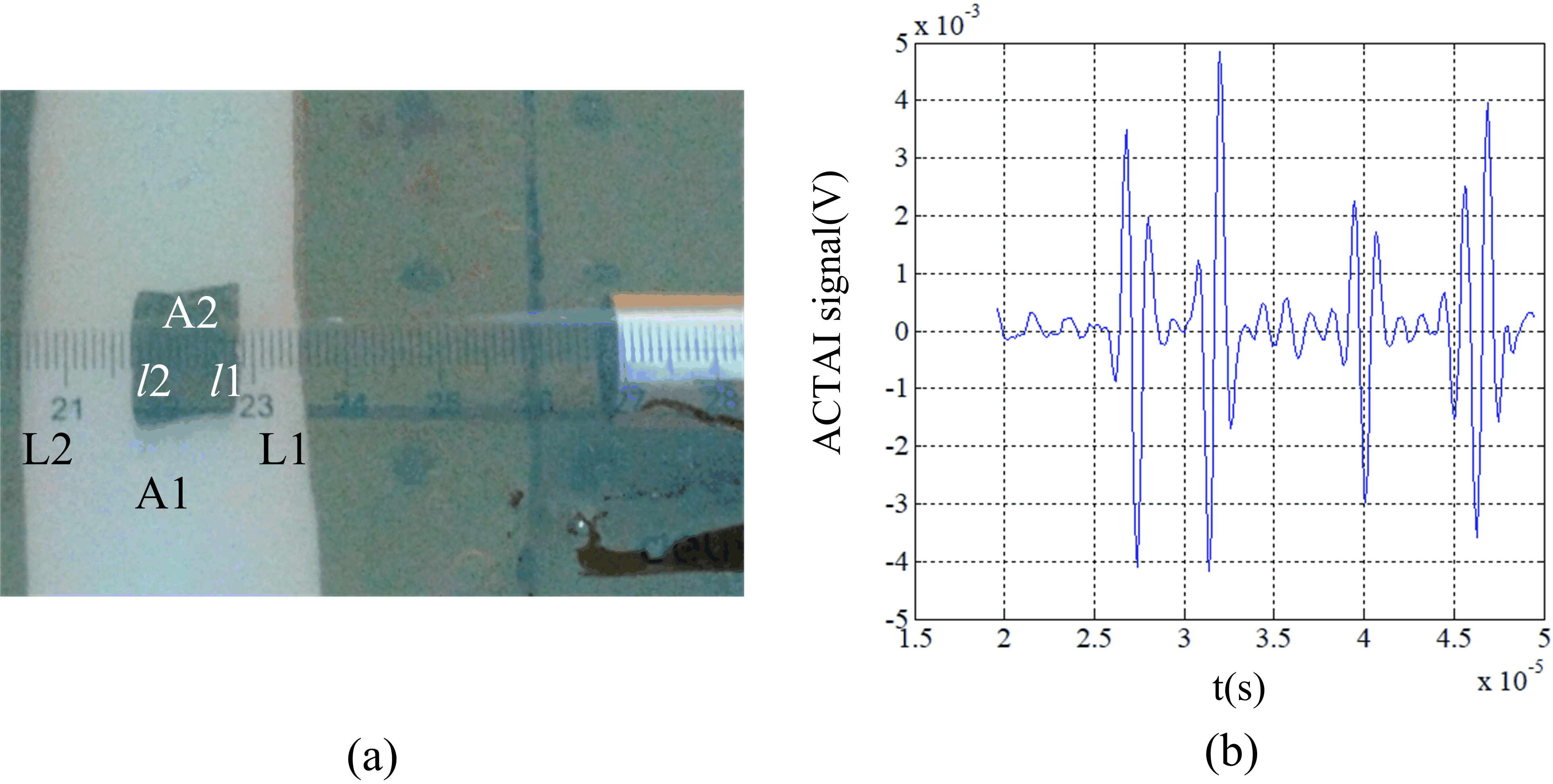
Figure 6.

Schematic diagram of the pork and the transducer.

In the experiments, the model was made of 10% cooled salinity gel as shown in Fig. 5. The phantom is buckled from the rectangular A1 model with a small rectangular A2. The length and width of A1 are 14 cm and 3 cm respectively. The length and width of A2 are 1.5 cm and 1 cm respectively. The distance between the boundary L1 of A1 and A2 is 0.7 cm. The distance between the boundary L2 of A1 and A2 is 1.3 cm. When the positional relationship between the phantom and the transducer is shown in Fig. 5a, the distance between the interface of the transducer and the boundary L1 of A1 is set to be 3.5 cm. The oscilloscope received the sound waveform shown in Fig. 5b. The horizontal axis and the vertical axis of the figure represent time (10 μs/div) and measured voltage, respectively. The transducer detected the sound pressure signal. There are four obvious wave clusters of the wave which begin around 25 μs and end at about 46 μs, matching the spaces from the two outer boundaries of the phantom to the position of the transducer. Its first wave cluster corresponds with the acoustic signal from the change boundary of conductivity from oil-L1 to the transducer. The second wave cluster occurs about 30 μs, corresponding with the acoustic signal from the change boundary of conductivity from l1-oil to the transducer. The third wave cluster occurs about 37 μs, corresponding with the acoustic signal from the change boundary of conductivity from oil-l2 to the transducer. The fourth wave cluster corresponds with the acoustic signal from the change boundary of conductivity from L2-oil to the transducer. The acoustic signal agrees with the propagation delay of the sound wave. It indicates that the waveform is generated by the experimental target, and this can display the change information of its conductivity.

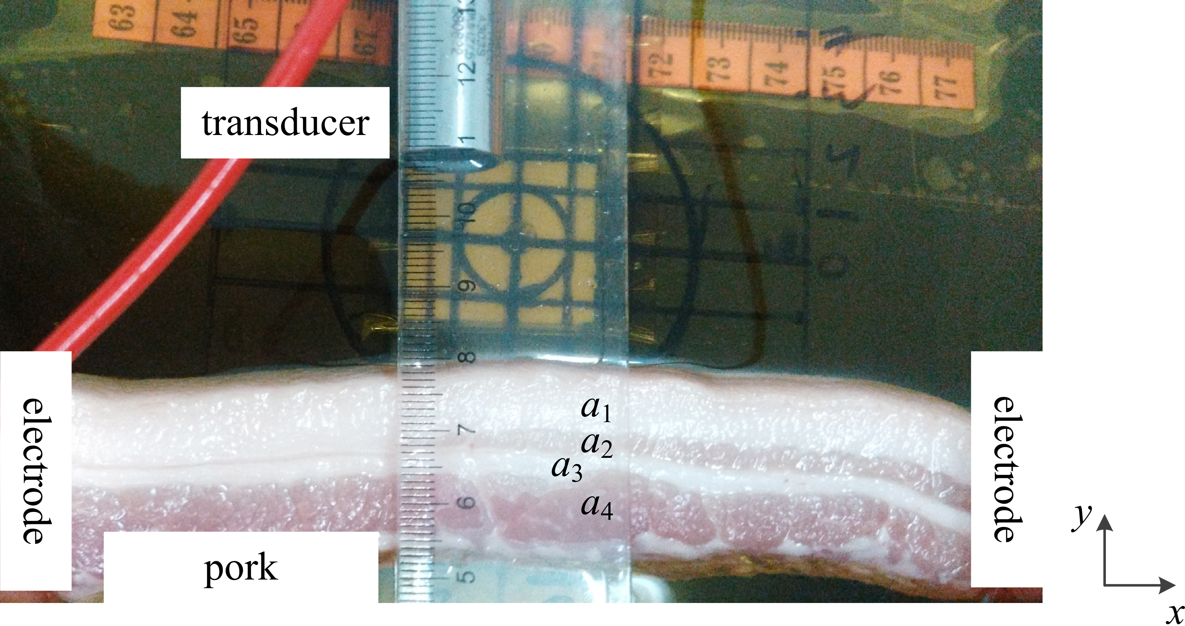
In the pork experiment, a piece of fresh pork was bought from a supermarket as the target. Figure 6 shows the positional relationship between the pork and the transducer. The length of the pork was about 2.5 cm in the y direction. The outer fat section a1 was about 1 cm length and the outer muscle section a4 was about 1 cm length in the y direction. The inner muscle section a2 and the inner fat section a3 were about 0.3 cm length in the y direction respectively. The conductivity of the fat tissue was very low around 0.02–0.03 S/m and the conductivity of the muscle was much higher about 0.55–0.62 S/m [28]. The distance between the interface of the transducer and the pork boundary close to the transducer was set to be 3.5 cm.

Figure 7.

Acoustic waveform from a piece of fresh pork.

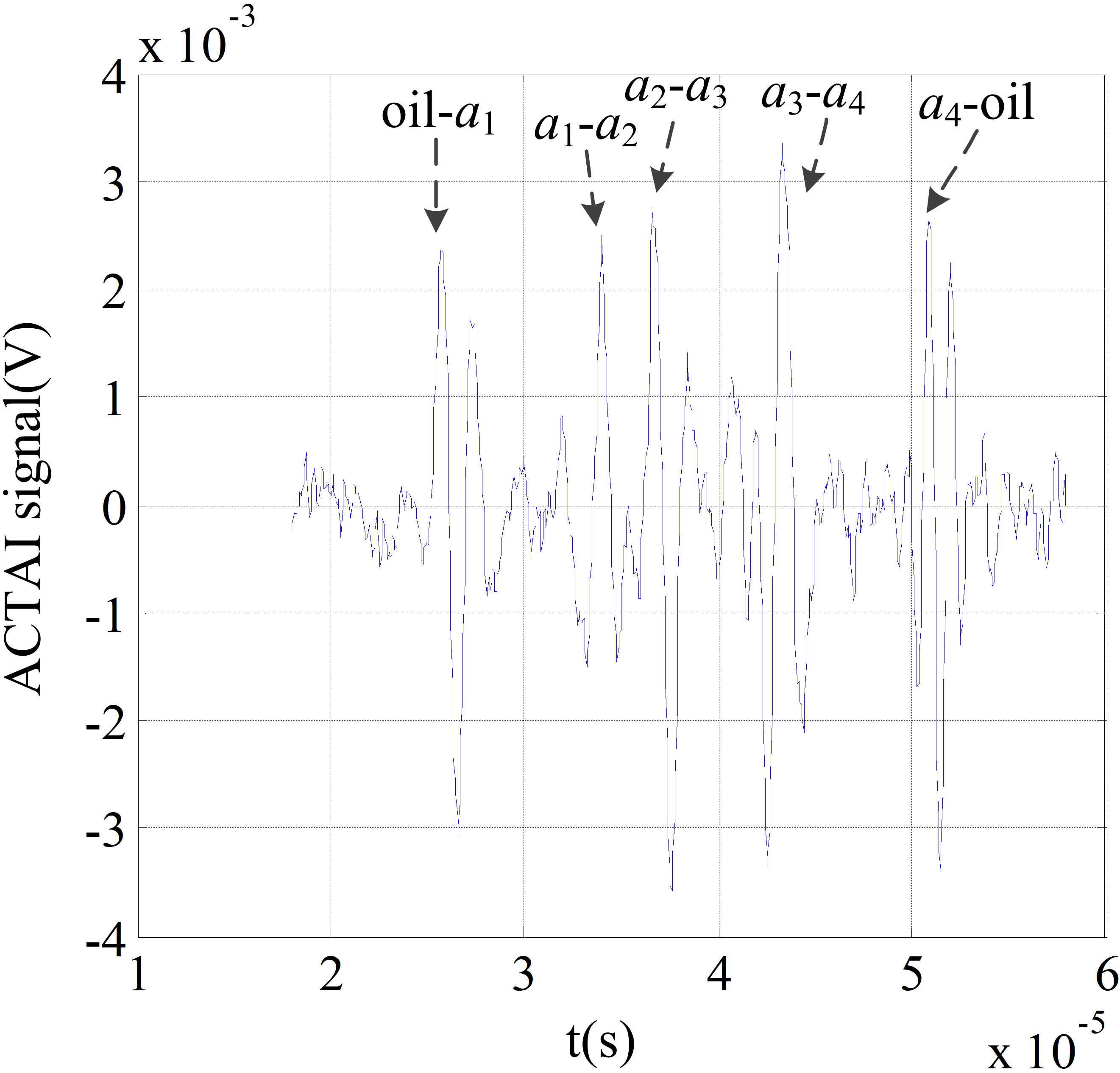
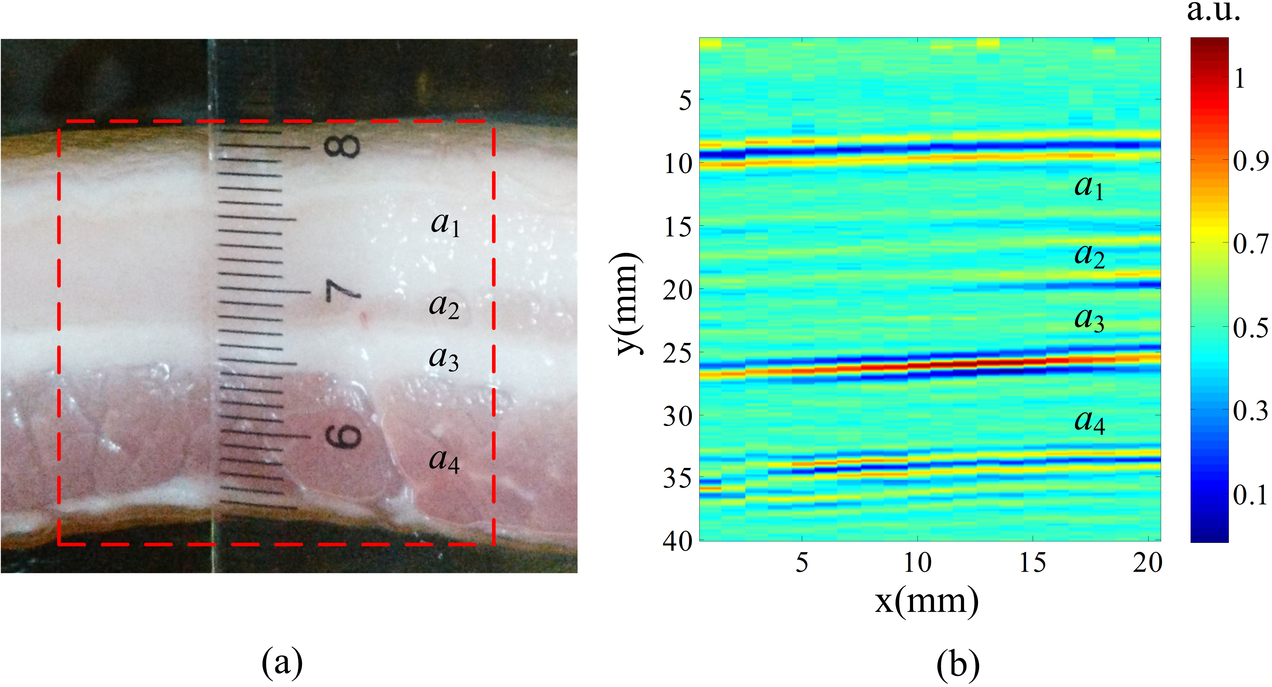
Figure 8.

Experimental results of fresh pork. (a) The imaging region. (b) B-scan ACTAI image with normalized scale of the tissue sample shown in (a).

The oscilloscope received the sound signal as shown in Fig. 7. The horizontal axis and the vertical axis of the figure represent time (10 μs/div) and measured voltage, respectively. There are five obvious wave clusters of the wave which begins around 25 μs and ends at about 44 μs, matching the distances from the two peripheral boundaries of the pork model to the position of the transducer. Its first wave cluster corresponds with the acoustic signal from the change boundary of conductivity from oil-a1 to the transducer. The second wave cluster corresponds with the acoustic signal from the change boundary of conductivity from a1-a2 to the transducer. The third wave cluster corresponds with the acoustic signal from the change boundary of conductivity from a2-a3 to the transducer. The fourth wave cluster corresponds with the acoustic signal from the change boundary of conductivity from a3-a4 to the transducer. And the last wave cluster corresponds with the acoustic signal from the change boundary of conductivity from a4-oil to the transducer. The acoustic signal agrees with the propagation delay of the sound wave. It indicates that the waveform is generated by the fresh pork target, and it can display the conductivity change information of the pork target.

The transducer is moved in the x direction from -10 mm to 10 mm in the step of 1 mm. The sample for imaging section is the red dashed box shown in Fig. 8a from Fig. 6. The B-scan image of this pork was produced from the collected acoustic signals as shown in Fig. 8b, which displays the changes conductivity information of the pork model with visible slanting fat-to-muscle interface and muscle-to-fat interface in good agreement with the real photograph of the pork model structure as shown in Fig. 8a. It displays that the boundary changes of the conductivity. The five x direction lines correspond to the five oil-fat-muscle-fat-muscle-oil interfaces. The lines reflect the changes from oil to a1, from a1 to a2, from a2 to a3, from a3 to a4, and from a4 to a5, respectively. The image also reflects the changes of half muscle and half fat in the a2 region. In addition, the signal wave clusters collected by the transducer as a result of the convolution between the sound pressure and the impulse response function of the transducer, the waveforms are generated from the abrupt pressure changes at conductivity boundaries. Consequently, the images have some artifacts and interface blurring.

5.Conclusion

The feasibility and performance of the newly proposed ACTAI method was verified by computer simulations and experiment researches in thermoacoustic imaging from noninvasive pressure measurements. The theoretical formulas of ACTAI have been derived under the assumption of acoustic homogeneity. Therefore, the detection system is needed to further improve in sensitivity, in order to facilitate the application of this method in biological imaging. However, the present simulation and experiment results show the feasibility and effectiveness of the proposed ACTAI in a practical setting. A numerical simulation on low conductivity phantom has been investigated and an experiment setup with fresh pork close to the real human tissues has been conducted. In the simulation study, the signals from a low conductivity model were conducted. In the experiment study, the acoustic signals and B-scan images of the fresh pork were presented. The fresh pork model experiment demonstrates the effectiveness of the proposed approach. These results of the simulation and experiment studies provide a new approach for conductivity reconstruction of thermoacoustic imaging, and present one novelty imaging modality for the diagnosis of early disease to deeper penetration. Further studies would be conducted to establish the performance of ACTAI in biological tissues.

References

[1] | Xu M, Wang L. Photoacoustic imaging in biomedicine. Rev. Sci. Instrum. (2006) ; 77: : 041101. |
[2] | Xu M, Xu Y, Wang L. Time-domain reconstruction algorithms and numerical simulations for thermoacoustic tomography in various geometries. Trans. Biomed. Eng. (2003) ; 50: : 1086-1099. |
[3] | Guo L, Li L, Dong F, et al. Non-equilibrium plasma jet induced thermo-acoustic resistivity imaging for higher contrast and resolution. Sci Rep. (2017) ; 7. |
[4] | Yang Y, Liu G, Li Y, et al. Conductivity reconstruction for magnetically mediated thermoacoustic imaging. Journal of Medical Imaging & Health Informatics. (2018) ; 8: : 66-71. |
[5] | Jeong JJ, Choi H. An impedance measurement system for piezoelectric array element transducers. Measurement. (2017) ; 97: : 138-144. |
[6] | Choi H, Yeom JY and Ryu JM. Development of a multiwavelength visible-range-supported opto-ultrasound instrument using a light-emitting diode and ultrasound transducer. Sensors. (2018) ; 18: : 3324. |
[7] | Wang X, Pang Y, Ku G. Noninvasive laser-induced photoacoustic tomography for structural and functional imaging of the brain. Nat. Biotech. (2003) ; 21: : 803-806. |
[8] | Wang L. Tutorial on photoacoustic microscopy and computed tomography. IEEE J. Sel. Top. Quantum Electron. (2008) ; 14: : 171-179. |
[9] | Lin H, Wei Q, Jin X, et al. Thermoacoustic tomography: A novel method formerly breast tumor detection. X-Acoustics: Imaging and Sensing. (2015) ; 1. |
[10] | Mashal A, Booske J, Hagness S. Toward contrast-enhanced microwave-induced thermoacoustic imaging of breast cancer: An experimental study of the effects of microbubbles on simple thermoacoustic targets. Phys. Med. Biol. (2009) ; 54: : 641-650. |
[11] | Choi H, Woo P, Yeom JY, et al. Power MOSFET linearizer of a high-voltage power amplifier for high-frequency pulse-echo instrumentation. Sensors. (2017) ; 17: : 764. |
[12] | Feng X, Gao F, Zheng Y. Magnetically mediated thermoacoustic imaging toward deeper penetration. Appl. Phys. Lett. (2013) ; 103: : 083704-083707. |
[13] | Feng X, Gao F, Zheng Y. Modulatable magnetically mediated thermoacoustic imaging with magnetic nanoparticles. App. Phy. Lett. (2015) ; 106: : 093705. |
[14] | Gabriel C, Corthout E. The dielectric properties of biological tissues: I. Literature survey. Phys. Med. Biol. (1996) ; 41: : 2231-2279. |
[15] | Gabriel S. Compilation of the dielectric properties of body tissues at RF and microwave frequencies. Phys. Med. Biol. (1996) ; 41: : 2251-2269. |
[16] | Fear E, Hagness S, Meaney P. Enhancing breast tumor detection with near-field imaging. Microwave Magazine IEEE. (2002) ; 3: : 48-56. |
[17] | Campbell A, Land D. Dielectric properties of female human breast tissue measured in vitro at 32 GHz. Physics in Medicine & Biology. (1992) ; 37: : 193-210. |
[18] | Zhou Y, Yao J, Wang L. Tutorial on photoacoustic tomography. Journal of Biomedical Optics. (2016) ; 21: : 61007. |
[19] | Wang S, Ma R, Zhang S, et al. Translational-circular scanning for magneto-acoustic tomography with current injection. Biomedical Engineering Online. (2016) ; 15: : 10. |
[20] | Payne B, Venugopalan V, Miki B, et al. Optoacoustic tomography using time-resolved interferometric detection of surface displacement. Journal of Biomedical Optics. (2003) ; 8: : 273-280. |
[21] | Hao N, Arbabian A. Peak-power-limited frequency-domain microwave-induced thermoacoustic imaging for handheld diagnostic and screening tools. IEEE Transactions on Microwave Theory & Techniques. (2017) ; 65: : 2607-2616. |
[22] | Yang Y, Xia Z, Li Y, et al. Reconstruction of acoustic source in applied current thermoacoustic imaging. Scientia Sinica. (2018) . |
[23] | Liu G, Huang X, Xia H, et al. Magnetoacoustic tomography with current injection. Science Bulletin. (2013) ; 58: : 3600-3606. |
[24] | Liu G. Magnetic Acoustic Imaging Technology: Magnetic Acoustic Imaging Based on Ultrasonic Detection, 1st ed. Beijing, China: Science Press; (2014) . |
[25] | Wang S, Ma R, Zhang S, et al. Translational-circular scanning for magneto-acoustic tomography with current injection. Biomedical Engineering Online. (2016) ; 15: : 10. |
[26] | Xu M, Wang L. Time-domain reconstruction for thermoacoustic tomography in a spherical geometry. IEEE Transactions on Medical Imaging. (2002) ; 21: : 814. |
[27] | Liu S, Zhao Z, Zhu X, et al. Block based compressive sensing method of microwave induced thermoacoustic tomography for breast tumor detection. Journal of Applied Physics. (2017) ; 122: : 7-1810. |
[28] | Hu G, et al. Imaging biological tissues with electrical conductivity contrast below 1 Sm-1 by means of magnetoacoustic tomography with magnetic induction. Appl. Phys. Lett. (2010) ; 97: : 103705. |