
Climate change scenario analysis in Spree catchment, Germany using statistically downscaled ERA5-Land climate reanalysis data1
Abstract
This study focuses on the statistical downscaling of ERA5-Land reanalysis data using the Statistical DownScaling Model (SDSM) to generate climate change scenarios for the Spree catchment. Linear scaling was used to reduce the biases of the Global Climate Model for precipitation and temperature. The statistical analyses demonstrated that this method is a promising and straightforward way of correcting biases in climate data. SDSM was used to generate climate change scenarios, which considered three emission scenarios: RCP 2.6, RCP 4.5, and RCP 8.5. The results indicated that higher precipitation is expected under higher emission scenarios. Specifically, the summer and autumn seasons were projected to experience up to 50 mm more rainfall in the next 80 years, and the temperature was projected to increase by up to 1∘C by 2100. These projections of climate data for different scenarios are useful for assessing water management studies for agricultural and hydrologic applications considering changing climate conditions. This study highlights the importance of statistical downscaling and scenario generation in understanding the potential impacts of climate change on water resources. The results of this study can provide valuable insights into water resource management, especially on adapting to changing climate conditions.
1.Introduction
In recent decades, the impacts of climate change have manifested prominently, characterized by a discernible rise in global temperatures [1, 2], accelerated ice melting in cold regions [3], rising sea levels [4, 5, 6, 7], heightened frequency of extreme weather occurrences [8, 9, 10], alterations in precipitation patterns [11, 12, 13, 14], ocean acidification [15, 16, 17], and diminished crop yields [18, 19, 20]. These documented consequences represent only a subset of the comprehensive array of effects associated with climate change, and their persistence is anticipated to further exacerbate the existing environmental challenges. Owing to the geographical heterogeneity of the Earth’s regions, the regional-level manifestation of these phenomena exhibits substantial variations across time and space.
To gain a deeper understanding of the potential impacts of climate change on various Earth processes, climate models [21] are commonly evaluated and utilized in several existing numerical models. They have proven to be valuable tools, provided that a thorough evaluation is conducted before incorporating them into numerical models. Climate model outputs act as drivers for numerical models that simulate various processes, including water balance [22], crop productivity [23], hydrological processes [24], watershed simulation [25], among others.
Understanding climate started with basic ideas (conceptual models [26]). In the 1800s, scientists used math to track energy flow and heat movement (energy balance/radiative transfer models [27]) and compare climates of different regions (analog models). Since the 1950s, powerful computers allowed detailed simulations of Earth’s overall air movement (global/general circulation models [28, 29]). Recently, models increasingly combine different parts of the climate system (coupled models [30]). Evaluating and comparing these models is leading to more standardized building blocks (modules), potentially uniting research and practical applications of climate science [31].
In contemporary hydrologic and agricultural research, Global Climate Models (GCMs) have garnered significant attention. Nonetheless, the majority of existing GCMs exhibit a coarse resolution, characterized by a horizontal cell size of approximately 100 km [32]. As a result, the use of such data for impact assessment in point-scale studies is impeded by the intrinsic biases of the climate models [33].
In order to address the existing limitations in using climate models, SDSM [34] was utilized to downscale GCM outputs to a finer resolution, making them more beneficial for regional-scale and even point-scale applications. The ERA5-Land reanalysis dataset [35], which could offer high-quality, high-resolution climate data for land areas, is one of the many available datasets that has proven particularly helpful for this purpose [36]. ERA5-Land offers a collection of reanalyzed historical records of how land features have changed from 1950 to present. This dataset is available in finer resolution than ERA5, with a horizontal grid dimension of 0.1∘
Statistical downscaling and climate change analysis are two examples of SDSM applications employing ERA5-Land data. This dataset can be used to create downscaled weather data that is deemed beneficial to run numerical models in the form of crop yield simulation and hydrologic modeling. Through the implementation of statistical downscaling, the simulation accuracy can be enhanced, showing its potential application in agricultural and hydrologic studies.
Furthermore, downscaled weather data from ERA5-Land can be used as input parameters for climate projection studies using the representative concentration pathways (RCPs). These climate change scenarios are produced by the Intergovernmental Panel on Climate Change (IPCC) to depict various amounts of projected greenhouse gas emissions. Researchers can better understand how climate change may affect agriculture and hydrology at regional scales by using downscaled meteorological data as input parameters for climate models under different RCP scenarios.
The overarching objective of this study is to evaluate the applicability of ERA5-Land data. To achieve this goal, the study has outlined three specific objectives: (1) to eliminate the biases that are inherent in global climate data, (2) to perform statistical downscaling of precipitation and temperature data, and (3) to generate stochastic weather data, considering various climate change scenarios.
In this study, we seek to investigate whether there exists a significant discrepancy between the weather station and the ERA5-Land reanalysis dataset at the location of the Kübschutz station. The null and alternative hypotheses are stated as follows:
• Ho: The true mean difference between the weather data collected from the weather station and the ERA5-Land reanalysis data is equal to 0.
• Ha: The true mean difference between the weather data collected from the weather station and the ERA5-Land reanalysis data is not equal to 0.
These hypotheses underpin the formulation of the specific objectives of this research. Following the rigorous testing of both the alternative and null hypotheses, subsequent steps involved comprehensive analyses which include bias-correction, statistical downscaling, and climate change scenario analysis. The results of this investigation hold significant importance, particularly in research studies employing ERA5-Land climate reanalysis data for the development of numerical models and the formulation of policies pertaining to water resource management.
2.Methodology
2.1Study area
Figure 1.
Climate condition in Kübschutz station from 1981 to 2020.
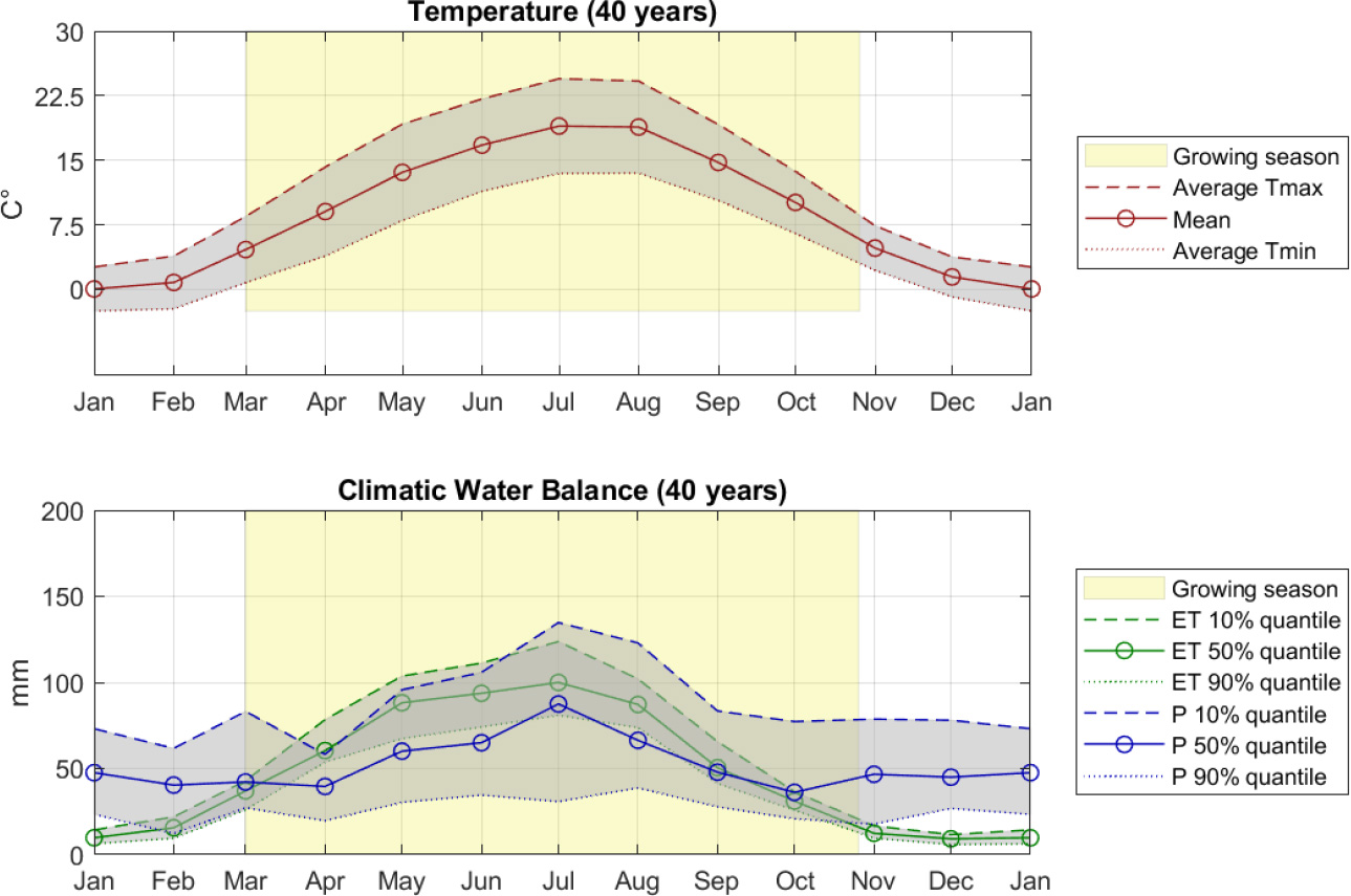
Saxony is situated in a humid westerly wind climate zone characterized by a cold or temperate climate. The study area exhibits a four-season climate regime (i.e., winter, spring, summer, and fall). The climatic conditions of the study area were assessed based on data obtained from the Kübschutz station over a period spanning from 1981 to 2020. The station data revealed that the mean annual temperature ranges from 5.4∘C to 13.7∘C. The minimum mean monthly temperature was observed in December (
2.2Data collection and evaluation
The data pertaining to the Spree Catchment utilized in this study were collected from diverse government and non-government online resources within Europe. The climate data from 1981 to 2020, such as rainfall and temperature, were sourced from the Deutscher Wetterdienst (DWD) [37].
For the purpose of this research, one weather station situated within the Spree catchment was chosen for further analysis. In the selection process, two weather stations in two major cities inside the Spree catchment were considered for evaluation: Bautzen station and Görlitz station. Historical daily time series data ranging from 1981 to 2020 for these two stations were downloaded from the Climate Data Center (CDC) of DWD. The meteorological parameters considered for evaluation were precipitation (mm) and maximum and minimum temperature (∘C) at 2 m above ground.
Table 1
Missing precipitation and temperature data from Kübschutz station
| Climate variable | Missing periods | Total number of missing data |
|---|---|---|
| Precipitation | 01 Sep 1998 to 30 Nov 1998 | 91 |
| Temperature | 01 Sep 1998 to 30 Nov 1998 07 Feb 2005 to 14 Feb 2005 25 Sep 2019 | 100 |
The downloaded weather data were thoroughly examined, and no missing values were observed for the Görlitz station. However, the Kübschutz Station exhibited a substantial amount of missing data (91 to 100) at different time periods. The dates during which the missing data were observed are listed in Table 1.
Given that modeling studies require continuous time series data, the missing values for precipitation and temperature at the Kübschutz station were estimated by leveraging data from neighboring stations. The method employed for imputing the missing weather data is elaborated upon in the subsequent section.
2.3Data processing
This research study encompassed the recovery and assessment of missing climate records, employing a range of methodologies to produce a historical climate dataset for the Kübschutz station. The techniques utilized to estimate missing climate data, rectify biases in the ERA5-Land dataset, and simulate time series data for climate change scenarios are elaborated below.
2.3.1Gap filling weather data
Various methods are used in hydrology to estimate missing climate data, such as arithmetic average (AA), inverse distance weighting (IDW), normal ratio, single best estimator (SIB), linear regression (LR), multiple linear regression analysis (MLR), multiple imputations (MI), non-linear iterative partial least squares (NIPALS) algorithm, UK traditional (UK), and decision tree model [38]. Sattari et al. (2017) conducted a study and found that simple AA provides the best estimate for missing climate data (R
(1)
where V0 denotes the predicted value of the missing data, Vi is the value of the same parameter at the ith nearest weather station, and N denotes the total number of nearby stations. If the gauges are evenly spaced out throughout the area and the individual gauge measurements do not significantly deviate from the mean, the AA approach is sufficient [40].
Figure 2.
Weather stations used to estimate missing precipitation and temperature data.
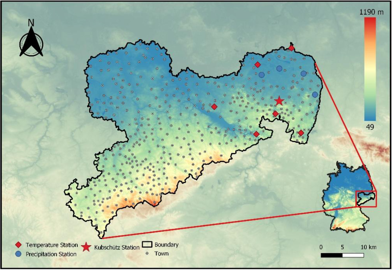
In this research, missing precipitation and temperature data were estimated using the Simple AA method. Figure 2 maps the neighboring stations that were utilized to approximate the missing temperature and precipitation data at the Kübschutz station. Specifically, four rain gauge stations were employed to estimate the missing precipitation data, while seven weather stations were utilized to estimate the missing temperature data.
2.3.2Quantifying percent bias of raw and corrected ERA5-Land data
Initial evaluation of the ERA5-Land data was conducted by quantifying the percent bias of the raw ERA5-Land data as compared to the generated historical data of the Kübschutz station. Percent bias (PBIAS) quantifies the average simulated data tendency to differ from the observed data by a given percentage [41]. With low-magnitude values indicating accurate model simulation, PBIAS should be optimized around 0.0. Gupta et al. [42]found that positive values represent model overerestimation bias and negative values represent model underestimation bias [42]. PBIAS is computed, using Eq. (2),
(2)
where PBIAS is the percentage bias of the model,
2.3.3Testing for significant difference between station and reanalysis data
The most popular method to compare the means of two groups and check if there exists a significant difference between the samples is the Student’s
(3)
2.3.4Bias-correcting ERA5-Land data
This study investigates the feasibility of utilizing global reanalysis datasets in agricultural and hydrological modeling in the Lusatia region. The meteorological data from ERA5-Land, including total precipitation and 2m temperature, were assessed. The data used in this study were obtained in NETCDF file format and had a time resolution of one hour. Climate Data Operators (CDO) [44] was employed to extract the time-series data. The daily maximum and minimum temperatures were extracted, while the time-series of total precipitation was created by extracting the data at 00:00 and lagged by one day.
Reanalysis projects involve reprocessing observational data from an extended historical period using a reliable and contemporary analysis system [45] to produce a dataset that can serve as a “proxy” for observations. The dataset provides coverage and time resolution that are often unachievable using traditional observational networks. The European Centre for Medium-Range Weather Forecasts (ECMWF) is currently working on an improved global dataset for the land component of the fifth generation of European ReAnalysis (ERA5) within the framework of the European Commission’s Copernicus Climate Change Service (C3S). The ERA5-Land model can be used for trend and anomaly analysis and can describe the water and energy cycle evolution over land.
Global and regional climate models often have systematic errors (biases), such as an overestimation of rainy days and an underestimation of extreme rainfall. Bias-correction methods, such as linear scaling, variance scaling, and local intensity scaling, were used to address issues related to the utilization of these data on modeling and impact studies in data-scarce regions. In this study, these methods were evaluated to correct the precipitation and temperature data obtained from the ERA5-Land reanalysis dataset.
Linear scaling method
In the linear scaling approach, the downscaling process involves computing the mean differences between monthly observed time series and the corresponding historical run time series of the Global Climate Model/Regional Climate Model for the same time period. These differences are then employed to correct for biases in climate simulation data and derive bias-corrected climatic variables. While temperature corrections follow an additive scheme, other variables such as precipitation, vapor pressure, and solar radiation require multiplicative corrections [46]. Equations (2.3.4) and (2.3.4) below are used for the linear scaling factor method:
(4)
(5)
where,
Variance scaling method
Chen et al. (2011) introduced the concept of utilizing a variance scaling approach [47]. Initially, the method involves applying linear scaling (as detailed in Eqs (2.3.4) and (2.3.4)) to modify the mean of the climate model. Subsequently, the mean-adjusted control run (
(6)
(7)
(8)
(9)
Then, based on the ratio of the observed
(10)
(11)
Finally, using the corrected mean and
(12)
(13)
The output of the climate model is compared to the observed data, and the results were used to scale the standard deviations. To finish the procedure, the mean that was corrected in step one was used to shift back the standard deviation corrected model run.
Local intensity scaling method
In this bias-correction method, the rainfall intensity threshold (Pthres,m) for each month was initially confirmed. As a result, the number of wet days in RCM precipitation that surpass this cutoff coincides with the days for which observed precipitation was calculated [48]. This method successfully gets rid of the drizzle effect because the original RCM outputs frequently include too many days with rain [49]. The mean amounts of corrected precipitation were then adjusted with a scaling factor (sm) to match observations. The mean of a rainfall time series can be changed, as well as the frequency and intensity of wet days [50, 51]. Shown in Eqs (14) and (15) are the formula used for LOCI scaling method:
(14)
(15)
where, s
2.3.5Climate change scenario generation
In this study, the effects of climate change on weather patterns were evaluated through the generation of synthetic weather data using GCMs developed under the assumption of three RCPs. According to GCMs, increasing greenhouse gas concentrations will have a significant impact on both the global and regional climate. Unfortunately, due to their coarse spatial resolution (typically of the order of 50,000 km2) and inability to resolve significant sub-grid scale features like clouds and topography, GCMs are not very useful for local impact studies [52].
To bridge the gap between GCM and numerical simulation studies, two approaches were developed to generate point-scale climate variables derived using regional scale atmospheric predictor variables: (1) statistical downscaling; (2) Regional Climate Models (RCMs).
Figure 3.
Schematic diagram adapted for the climate scenario generation using SDSM Version 4.2.
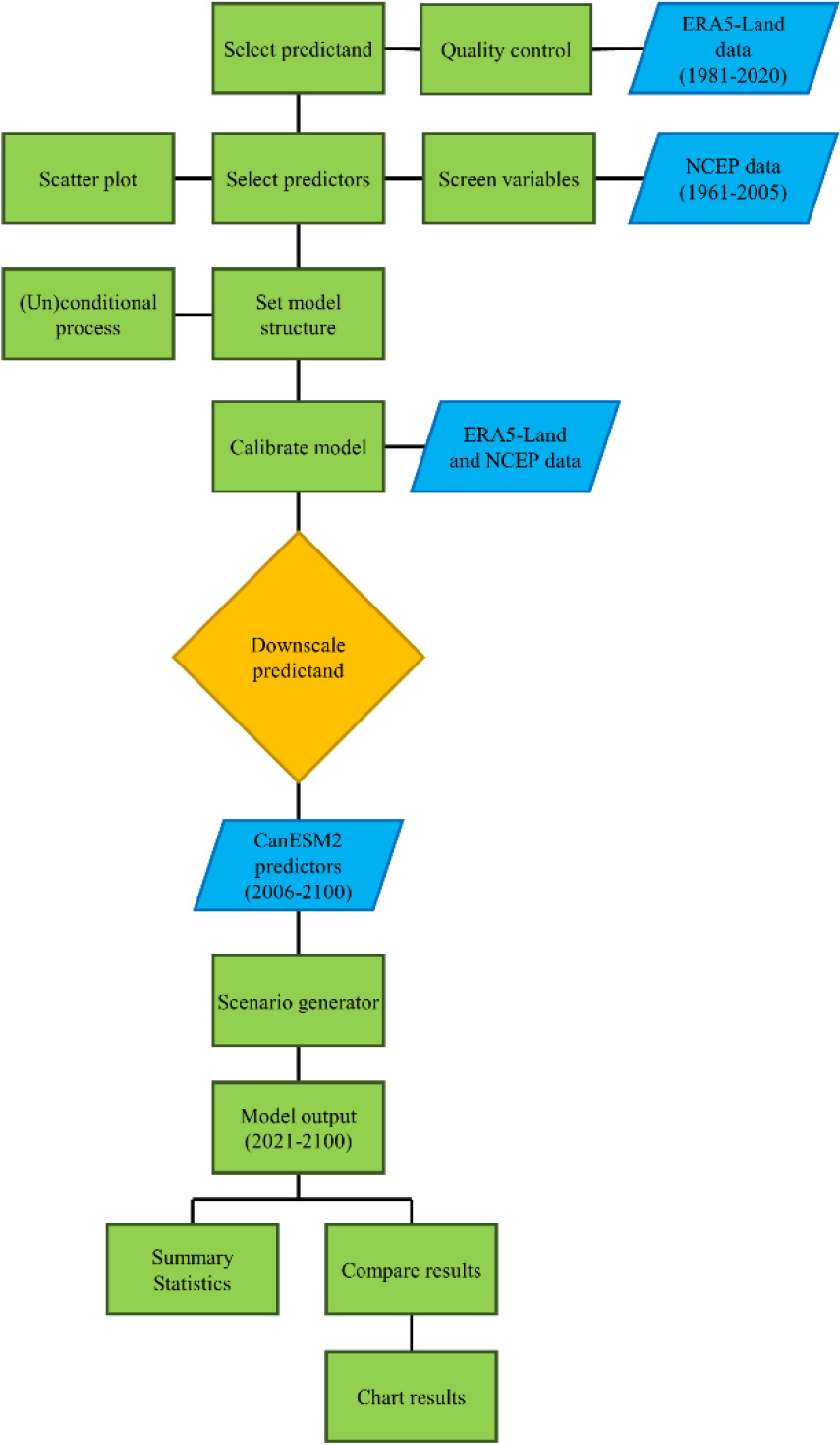
In this study, SDSM version 5.3 was utilized to understand the climate change impacts on future climate trends. This model was used to create the necessary point-scale resolution climate projection by establishing a statistical correlation between the large- and point-scale climate variables [53]. Due to its applicability and better performance compared to other statistical downscaling models, it is now one of the most used statistical downscaling models. Illustrated in Fig. 3 is the schematic diagram followed to generate climate data for the three RCP pathways. These scenarios range from a low emission scenario with active mitigation (RCP 2.6), an intermediate scenario (RCP 4.5), to a high emission scenario (RCP 8.5).
To meet the previously established goal of assessing the impact of climate change scenarios on weather patterns, the ensemble of daily predictor variables created by the Canadian Earth System Model (CanESM2) – Coupled Model Intercomparison Project Phase 5 (CMIP5) experiment was used as input files for the model. This input data includes long-term time-series data of NCEP-NCAR (2006–2100) and CanESM2 (1961–2100). Standardized daily values over an extended time series are compiled into individual one-column text files for each grid cell (box). The global domain is represented by a 128
For the purpose of calibration, the 26 NCEP-NCAR predictors were used. The predictors were screened using linear correlation analysis between the predictand and the 26 predictor variables.
Using the bias-corrected ERA5-Land data, and the selected predictor variables, calibration was done on a monthly basis. This step allows the computation of the parameters of multiple regression equations using the dual simplex optimization algorithm.
Table 2
Percent bias (PBIAS) comparison between weather station data and raw/corrected ERA5-Land reanalysis data
| Weather variable | DWD vs. | |||
|---|---|---|---|---|
| ERA5-Land | Linear scaling | Local intensity scaling | Variance scaling | |
| Rainfall | 26.4 | 0 | 20.1 | – |
| Maximum temperature | –7.3 | 0 | – | 0 |
| Minimum temperature | 5.4 | 0 | – | 0 |
Note:
3.Results and discussion
3.1Kübschutz station vs. ERA5-Land data
A comparative analysis was conducted to quantify the Percent Bias (PBIAS) of ERA5-Land reanalysis data against the station data for rainfall, maximum temperature, and minimum temperature (Table 2). PBIAS served as the evaluation metric to see how effective different bias-correction methods are in minimizing the discrepancy between the station and the ERA5-Land reanalysis dataset. Evaluation of bias-correction techniques were done by comparing the downloaded data before and after implementing two correction methods: linear scaling and local intensity scaling for rainfall, and linear scaling and variance scaling for temperature.
For rainfall, the raw ERA5-Land data revealed a substantial overestimation bias of 26.4%. Linear scaling correction successfully negated this bias, achieving a PBIAS of 0%. However, local intensity scaling, while minimizing the gap, left a noticeable bias of 20.1%, which shows an unsatisfactory performance of this method. The results highlight the varied effectiveness of the two correction methods across precipitation variables.
For maximum temperature, the uncorrected data exhibited an underestimation bias of
These findings underscore the significance of performing bias-correction techniques to ERA5-Land climate reanalysis datasets to enhance its accuracy. This is particularly crucial for hydrological and climatological studies which employ climate data in its numerical simulation. Additionally, the results emphasize the need for selecting the appropriate bias-correction method, as correction effectiveness varies depending on the meteorological variable.
3.2Two-sided student’s t
Table 3
Paired
| Weather variable | DWD vs. | |||
|---|---|---|---|---|
| ERA5-Land | Linear scaling | Local intensity scaling | Variance scaling | |
| Rainfall |
| |||
| Maximum temperature | 92.6** | – | ||
| Minimum temperature | 1.3e-13 | – | 1.1e-13 | |
Note: ** P-value
To test whether there is a significant difference between the weather station data and the raw/corrected ERA5-Land reanalysis data, Student’s
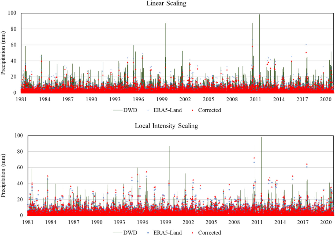
Figure 4.
Comparison of bias-corrected precipitation data using linear scaling and local intensity.
The results of the student’s
The linear scaling method for precipitation yielded a relatively small absolute
Looking at the result of the test, it is notable that all climate data from ERA5-Land exhibited significant difference from the station data, highlighting the need for bias-correction before incorporating such data into numerical models.
Using the linear scaling method on rainfall data yielded satisfactory results, as reflected in a
The results for maximum and minimum temperature data were unsatisfactory, indicated by a
3.3Bias-correction
3.3.1Precipitation
Figure 4 illustrates the precipitation time-series data in Kübschutz station. Comparison between the station data, ERA5-Land data, and bias-corrected data was presented from this illustration. The bias-corrected data through linear scaling method showed that station data has multiple precipitation measurements that are higher than the ERA5-Land reanalysis and bias-corrected data. On the other hand, the time-series data generated using local intensity scaling are relatively closer to the station data.
Table 4
Summary statistics of station, reanalysis, and bias-corrected precipitation data
| Summary statistics | DWD | ERA5-Land | Linear scaling | LOCI |
|---|---|---|---|---|
| Mean | 1.79 | 2.26 | 1.79 | 2.14 |
| Median | 0.00 | 0.69 | 0.54 | 0.00 |
| Mode | 0.00 | 0.00 | 0.00 | 0.00 |
| Standard deviation | 4.32 | 3.87 | 3.17 | 4.01 |
To provide a numerical comparison between the four precipitation data, the summary statistics were computed (Table 4). The long-term mean precipitation of the station was 1.79 mm. This value is equal to the computed mean of the bias-corrected precipitation data using linear-scaling method. Comparing the mean of the ERA5-Land reanalysis data, it was found that the mean was 0.47 mm higher than the station data. Although the local intensity scaling method appeared to have closer values to the station data, it was found that the mean precipitation generated using this method is 0.35 mm higher than the station data. Based on this numerical comparison, it was verified that the bias-corrected data using linear scaling method produces results that have similar mean with the station data. However, it was not able to generate extreme precipitation values as shown by the lowest maximum precipitation data among the four datasets compared.
Table 5
Correlation matrix of precipitation data
| DWD | ERA5-Land | Linear scaling | LOCI | |
|---|---|---|---|---|
| DWD | 1 | |||
| ERA5 | 0.6903 | 1 | ||
| Linear scaling | 0.6915 | 0.9948 | 1 | |
| LOCI | 0.6898 | 0.9919 | 0.9982 | 1 |
Figure 5.
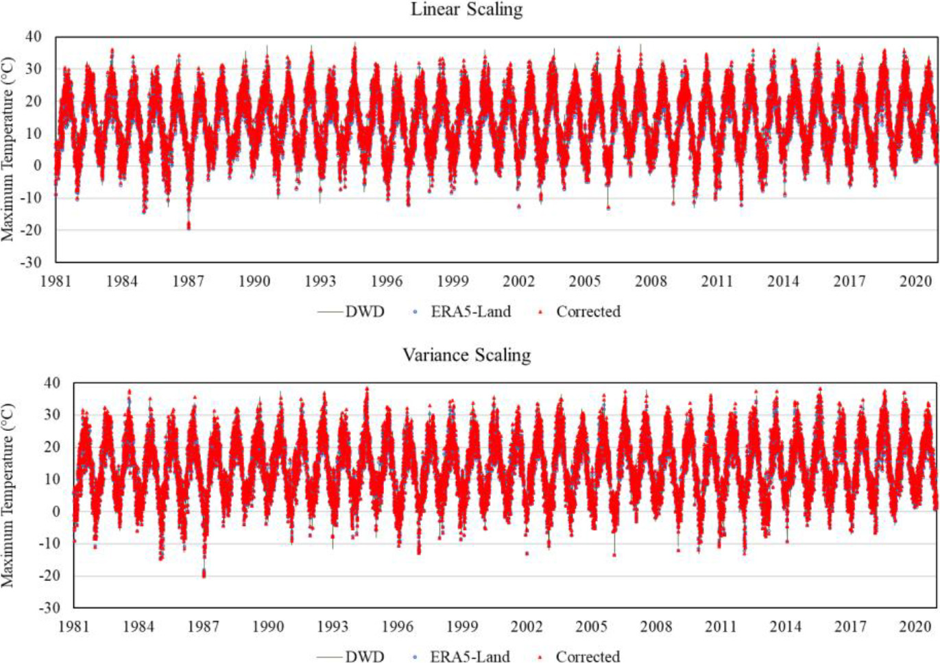
Comparison of bias-corrected maximum temperature data using linear scaling and variance.
In selecting the precipitation data that will be used for the simulation part of the study, linear correlation between the datasets were done. Presented in Table 5 is the correlation matrix of the precipitation data. Since, linear scaling method got higher correlation coefficient than the local intensity scaling method, the precipitation data corrected via linear scaling method was used.
3.3.2Maximum temperature
Figure 5 is a representation of the maximum temperature time-series data that was collected at the Kübschutz station. This illustration presents a comparison between the data from the stations, the data from ERA5, and the bias-corrected data. The bias-corrected data using linear scaling and the variance scaling approach both exhibited an excellent fit to the station data, in contrast to the precipitation data.
Table 6
Summary statistics of station, reanalysis, and bias-corrected maximum temperature data
| Summary statistics | DWD | ERA5-Land | Linear scaling | Variance scaling |
|---|---|---|---|---|
| Mean | 13.69 | 12.70 | 13.69 | 13.69 |
| Median | 13.80 | 12.94 | 13.87 | 13.82 |
| Mode | 8.00 | 13.81 | 20.52 | 20.33 |
| Standard deviation | 9.19 | 8.65 | 8.99 | 9.19 |
Table 7
Correlation matrix of maximum temperature data
| DWD | ERA5-Land | Linear scaling | Variance scaling | |
|---|---|---|---|---|
| DWD | 1 | |||
| ERA5 | 0.9912 | 1 | ||
| Linear scaling | 0.9911 | 0.9996 | 1 | |
| Variance scaling | 0.9914 | 0.9996 | 0.9992 | 1 |
The results of the computations for the summary statistics of the maximum temperature records are presented in Table 6. The station recorded a long-term mean maximum temperature of 13.69∘C. This result corresponds exactly to the computed mean of the bias-corrected data obtained by either method. When compared to the mean of the ERA5-Land reanalysis data, it was discovered that, on average, the ERA5-Land data is 0.99∘C off in its estimation of the maximum temperature data. On the basis of this numerical comparison, it was established that the bias-corrected data produced results that had a similar mean when compared with the station data. On the other hand, it was unable to produce extreme temperature values that were even remotely comparable to the station data.
The correlation matrix for the maximum temperature data can be found in Table 7. According to the summary statistics of the bias-corrected maximum temperature data, it was discovered that there was not a significant difference between the outcome of the linear scaling technique and the variance scaling approach. This was the conclusion reached after comparing the two methods. As a result, the maximum precipitation data that was bias-corrected using the linear scaling method were also utilized for the simulation study.
Table 8
Summary statistics of station, reanalysis, and bias-corrected minimum temperature data
| Summary statistics | DWD | ERA5-Land | Linear scaling | Variance scaling |
|---|---|---|---|---|
| Mean | 5.45 | 5.74 | 5.45 | 5.45 |
| Median | 5.80 | 6.08 | 5.81 | 5.79 |
| Mode | 0.00 | 11.27 | 9.16 | 9.33 |
| Standard deviation | 7.09 | 7.24 | 6.89 | 7.09 |
Table 9
Correlation matrix of minimum temperature data
| DWD | ERA5-Land | Linear scaling | Variance scaling | |
|---|---|---|---|---|
| DWD | 1 | |||
| ERA5 | 0.9720 | 1 | ||
| Linear scaling | 0.9729 | 0.9991 | 1 | |
| Variance scaling | 0.9721 | 0.9966 | 0.9988 | 1 |
Figure 6.
Comparison of bias-corrected minimum temperature data using linear scaling and variance scaling method.
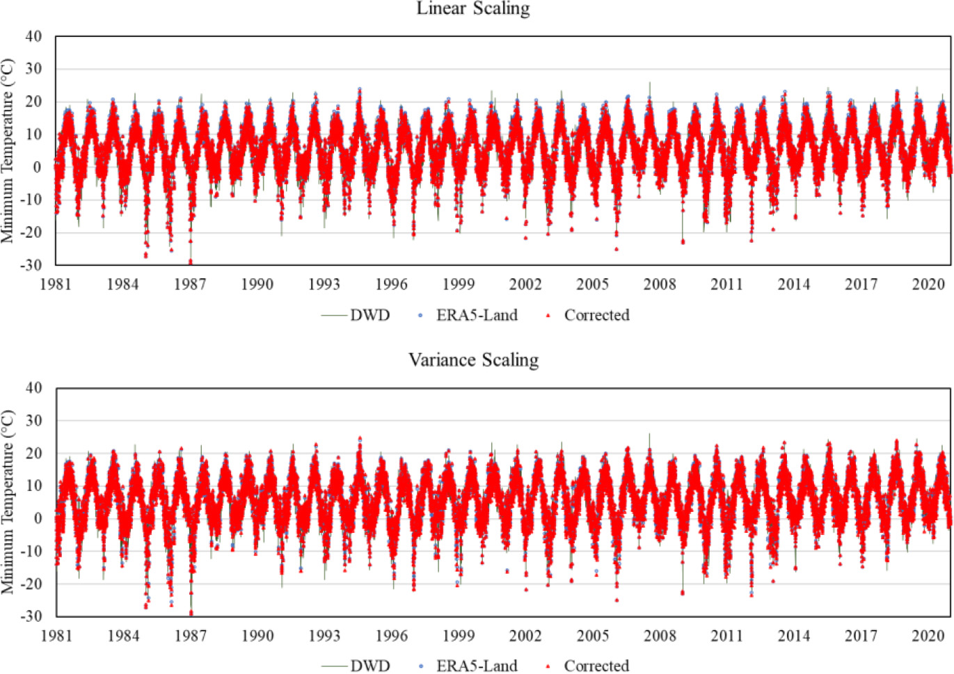
3.3.3Minimum temperature
A representation of the minimum temperature time-series data that was collected at the Kübschutz station can be found in Fig. 6. This diagram provides a comparison of station data, ERA5-Land data, and the bias-corrected data. A good fit can be seen between the bias-corrected data and the station data when the two bias-correction approaches are used. These results are comparable to the figures that were provided for the maximum temperature.
The outcomes of the calculated summary statistics of the minimum temperature records are shown in Table 8. A long-term mean low temperature of 5.45∘C was recorded at the station. This outcome matches the calculated mean of the bias-corrected data acquired using either method to an exact degree. It was observed that the ERA5-Land data were only 0.29∘C higher than the station data. The bias-corrected data generated time-series data with a mean that was comparable to the station data. Similar to the findings in the maximum temperature data, it was unable to generate extreme minimum temperature values that were close to the station data.
Table 9 contains the correlation matrix for the data on the minimum temperature. The linear scaling strategy was chosen after taking the correlation coefficient between the station data and the bias-corrected data into consideration.
3.4Selection of climate predictors
Table 10
Selected predictors for the statistical downscaling of CanESM2 RCP scenarios
| Predictor | Precipitation (mm) | Maximum temperature (∘C) | Minimum temperature (∘C) |
|---|---|---|---|
| 500 hPa vorticity |
|
| |
| 500 hPa geopotential height |
|
|
|
| 850 hPa specific humidity |
|
|
|
| 2 m mean temperature |
| ||
| 1000 hPa relative vorticity of true wind |
| ||
| 850 hPa geopotential height |
|
| |
| Total precipitation |
| ||
| 500 hPa specific humidity |
|
| |
| Surface specific humidity |
| ||
| Air temperature |
Climate predictors were selected from the 26 NCEP-NCAR predictors through correlation analysis. The four predictands (precipitation, maximum temperature, minimum temperature, and potential evapotranspiration) were each correlated to the available predictors. Predictor-predictand relationship which obtained a
3.5Climate change scenario generation
SDSM model inputs were bias-corrected data from ERA5-Land reanalysis data for the years 1981 to 2020. Following the selection of predictors and calibration, data is created for three scenarios (RCP 2.6, RCP 4.5, and RCP 8.5) for the years 2021–2100, day by day, for four variables (precipitation, maximum temperature, minimum temperature, and potential evapotranspiration). The results of climate variable predictions are discussed below.
Figure 7.
Monthly and seasonal changes in precipitation under future greenhouse gas forcing.
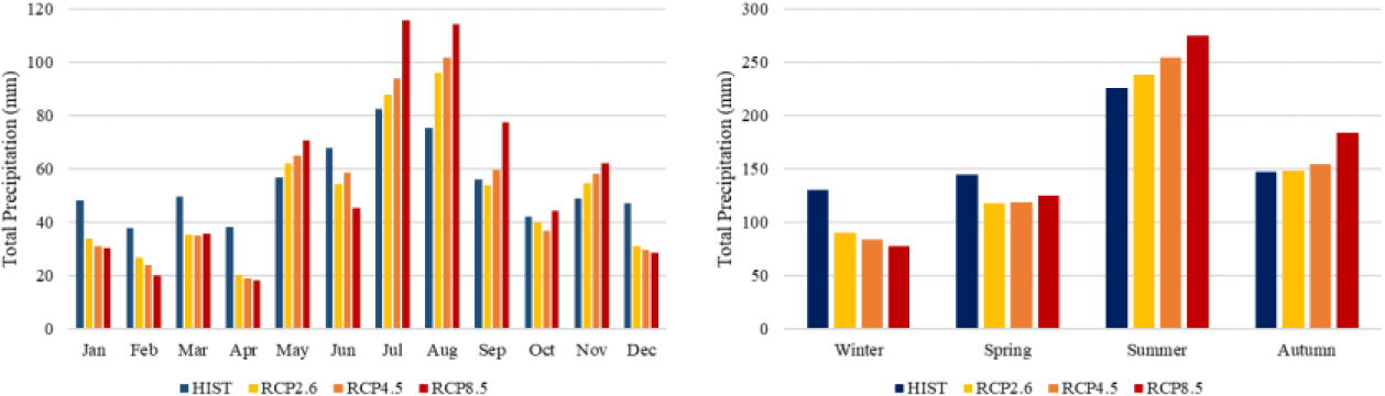
Depicted in Fig. 7 are the monthly and seasonal total precipitation values in the Spree catchment. The precipitation trend in the future varies seasonally. During winter season, a decreasing trend in total precipitation was observed from the low emission scenarios characterized by active mitigation (RCP 2.6), medium scenarios (RCP 4.5), and high emission scenarios (RCP 8.5). Conversely, the precipitation from spring season until autumn season increased from RCP 2.6 to RCP 8.5, respectively. The highest precipitation recorded from the generated data was during the summer season. This indicates more pronounced rainfall during this season than the other season. Comparing the projected precipitations to the ERA5-Land data, it was evident that lower precipitation is expected during winter and spring season in the next 80 years. On the other hand, increasing precipitation trend is expected during the summer and autumn season. Considering the monthly precipitation pattern, results showed that the highest precipitation is expected in the months of July and August while the lowest is in the month of April.
Figure 8.
Monthly and seasonal changes in mean maximum temperature future greenhouse gas forcing.
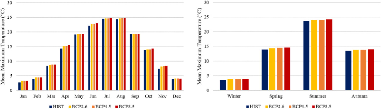
The monthly and seasonal mean maximum temperature data for the study area are shown in Fig. 8. It is anticipated that the mean maximum temperature will rise over the course of the year. The increase in the mean maximum temperature is less noticeable than the increase in precipitation trend as discussed earlier. Summer will likely experience the greatest temperature increase (1.26∘C higher than the historical norm). Under RCP 8.5, August had the highest simulated mean monthly maximum temperature (24.87∘C). As a result of this finding, it is anticipated that the area will see warmer temperatures than usual. As more evaporation takes place at higher temperatures, the rising trend in precipitation from spring to autumn may be linked to this. A greater annual maximum temperature is anticipated during the next 80 years when comparing the projected precipitation to the ERA5-Land data. Results indicated that based on the pattern of monthly mean maximum temperatures, the months of July and August are projected to have the largest precipitation amounts, while January is predicted to have the lowest temperature.
Figure 9.
Monthly and seasonal changes in mean minimum temperature under future greenhouse gas forcing.
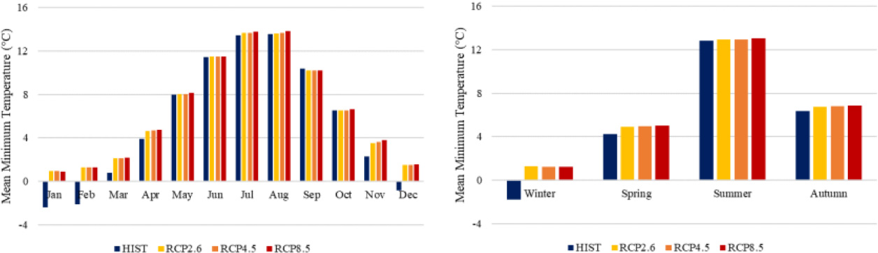
Figure 9 displays the mean minimum temperature data on a monthly and seasonal basis. It was projected that the mean minimum temperature would increase during the year, following the same pattern seen in the forecast mean maximum temperature. Particularly during the winter months, the increase in the mean minimum temperature was more evident (i.e., the mean minimum temperature in the next 80 years was projected to be positive unlike the historical data from 1981 to 2020). The greatest simulated mean monthly minimum temperature under RCP 8.5 scenario was recorded in August (13.86∘C), while the lowest was in January (0.90∘C). It is projected that the region will see higher temperatures than usual, particularly during the winter months. This could portend thinner snow in the frigid regions in the future. In comparison to historical data, a higher annual minimum temperature is predicted for the next 80 years. The months of July and August are anticipated to have the highest mean minimum temperatures, while January is anticipated to have the lowest mean minimum temperatures, following the monthly trend of mean maximum temperatures.
Figure 10.
Monthly and seasonal changes in total potential evapotranspiration under future greenhouse gas forcing.
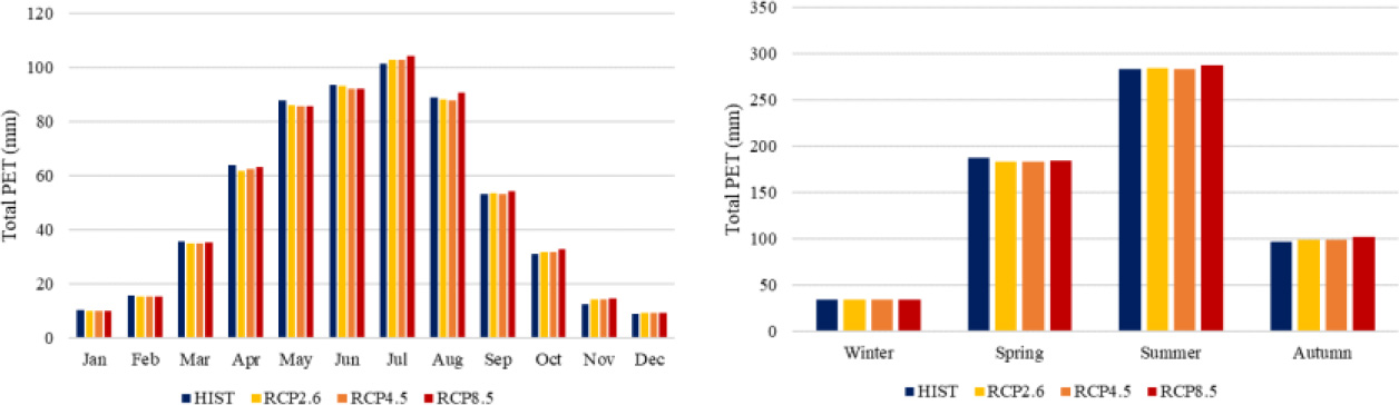
Shown in Fig. 10 are the monthly and seasonal changes in total evapotranspiration under gas forcing scenarios. Based on the monthly total PET, an increasing trend was observed in the months of March, April, June, and August until December. Conversely, the opposite trend was observed in the months of May and June. The varying trend observed for the PET variable can be attributed to the trend in monthly temperature and precipitation values as discussed earlier. The seasonal summary of PET indicates that maximum PET was observed in the summer season and lowest during the colder months of the winter season.
Figure 11.
Monthly and seasonal mean dry and wet spell length under future greenhouse gas forcing.
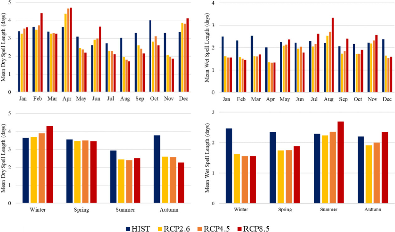
Considering the present climate change and fluctuation, knowledge of the distribution of wet and dry periods is essential for determining the start, end, and length of the growing season [55]. These spells are the most accurate proxies for identifying crop water stress and timing because they are strongly related to the local water balance [56]. The mean dry spell and wet spell lengths were calculated to better understand this occurrence under various climate change scenarios. Figure 11 shows the seasonal and monthly trend for the average length of a dry and wet spell. The figures show that the average lengths of dry and wet spells are inversely related to one another. It was predicted that the length of dry spells will lengthen throughout the winter months over the next 80 years on a seasonal basis. On the other hand, using historical data, a sudden fall in the mean dry spell length was modelled for the autumn season. The rising trend in mean wet spell length reflects the increase in total precipitation during the summer. According to the monthly values, the mean dry spell length is predicted to be higher in April and lower in August. On the other hand, the mean length of a wet spell is greatest in August and lowest in April.
4.Conclusions
The present study focuses on the statistical downscaling of ERA-Land reanalysis data using the SDSM tool to generate climate change scenarios for the Spree catchment, a crucial area for the management of both surface and groundwater systems in the Lusatia region. The primary objective of this research is to apply statistical downscaling for agricultural data and evaluate different bias-correction methods for precipitation and temperature time series data. Furthermore, the impact of different CO2 emission scenarios on the availability and accessibility of water resources in the future was also assessed.
As climate data is a critical input for hydrologic and agricultural models, the missing precipitation and temperature values in the time-series data were imputed through the arithmetic average method using climate data from the surrounding weather stations. The ERA5-Land reanalysis data was utilized in this study, and linear-scaling was employed to minimize the biases of the GCM for precipitation and temperature data. The statistical analyses demonstrated that linear scaling is a promising and straightforward approach to correct the biases in climate data.
SDSM was employed to generate climate change scenarios, considering three emission scenarios: active mitigation (RCP 2.6), medium emission (RCP 4.5), and high emission (RCP 8.5). The results of the scenario generation revealed that higher precipitation is expected under higher emission scenarios. Specifically, the summer and autumn seasons are projected to experience up to 50 mm more rainfall in the next 80 years. The temperature is also projected to increase by up to 1 degree Celsius by 2100. These projections of climate data for different scenarios are useful in assessing water management studies for agricultural and hydrologic applications considering changing climate conditions.
5.Recommendations
The downscaling model has proven effective in replicating high-resolution climate patterns from coarse-scale data. Despite this success, there are critical areas for future improvement. One point of improvement involves leveraging ancillary geospatial data, such as digital elevation models and land cover information, to enhance downscaling accuracy. The incorporation of these additional layers could provide valuable insights for refining the model and introducing spatial stratification, ultimately contributing to a more nuanced representation of local conditions.
Furthermore, the consideration of spatial effects, including spatial autocorrelation, is of greatest importance for advancing model accuracy. Integrating spatial dependencies can capture intricate relationships between neighboring regions, leading to a more realistic portrayal of local climate variations. Lastly, to ensure the reliability of downscaled data, rigorous validation procedures are essential. Future research should focus on comprehensive validation, comparing downscaled results with observed high-resolution climate data, and conducting sensitivity analyses to assess the model’s robustness under various scenarios. Addressing these aspects will drive forward downscaling methodologies, yielding more accurate and reliable high-resolution climate projections in future studies.
Acknowledgments
The author extends sincere appreciation to Dr. Niels Schuetze from Technische Universität Dresden for his invaluable guidance and expertise, which significantly contributed to the completion of this research during the Erasmus Mundus Joint Master Program in Groundwater and Global Change – Impacts and Adaptation. Immense gratitude is also expressed to the World Bank for sponsoring the author’s participation in the Ninth International Conference on Climate Change, where this research study was initially presented. Lastly, acknowledgment is extended to the UPLB Academic Development Fund for Faculty for their support in funding the author’s Visa application.
References
[1] | Zandalinas SI, Fritschi FB, Mittler R. Global warming, climate change, and environmental pollution: Recipe for a multifactorial stress combination disaster. Trends in Plant Science [Internet]. (2021) ; 26: (6): 588-99. Available from: doi: 10.1016/j.tplants.2021.02.011. |
[2] | Crowley TJ. Causes of climate change over the past 1000 years. Science [Internet]. (2000) ; 289: (5477): 270-7. Available from: doi: 10.1126/science.289.5477.270. |
[3] | Colucci RR, Guglielmin M. Climate change and rapid ice melt: Suggestions from abrupt permafrost degradation and ice melting in an alpine ice cave. Progress in Physical Geography: Earth and Environment [Internet]. (2019) ; 43: (4): 561-73. Available from: doi: 10.1177/0309133319846056. |
[4] | Mimura N. Sea-level rise caused by climate change and its implications for society. Proceedings of the Japan Academy Series B Physical and Biological Sciences [Internet]. (2013) ; 89: (7): 281-301. Available from: doi: 10.2183/pjab.89.281. |
[5] | Chen C-C, McCarl B, Chang C-C. Climate change, sea level rise and rice: global market implications. Climatic Change [Internet]. (2012) ; 110: (3–4): 543-60. Available from: doi: 10.1007/s10584-011-0074-0. |
[6] | Milne GA, Gehrels WR, Hughes CW, Tamisiea ME. Identifying the causes of sea-level change. Nature Geoscience [Internet]. (2009) ; 2: (7): 471-8. Available from: doi: 10.1038/ngeo544. |
[7] | Swapna P, Ravichandran M, Nidheesh G, Jyoti J, Sandeep N, Deepa JS, et al. Sea-Level Rise. In: Assessment of Climate Change over the Indian Region. Singapore: Springer Singapore. (2020) ; 175-89. |
[8] | Meehl GA, Zwiers F, Evans J, Knutson T, Mearns L, Whetton P. Trends in extreme weather and climate events: Issues related to modeling extremes in projections of future climate change*. Bulleting of the American Meteorological Society [Internet]. (2000) ; 81: (3): 427-36. Available from: doi: 10.1175/1520-0477(2000)081<0427:tiewac>2.3.co;2. |
[9] | National Academies of Sciences, Engineering, and Medicine, Division on Earth and Life Studies, Board on Atmospheric Sciences and Climate, Committee on Extreme Weather Events and Climate Change Attribution. Attribution of extreme weather events in the context of climate change. Washington, D.C., DC: National Academies Press; (2016) . |
[10] | Jentsch A, Kreyling J, Beierkuhnlein C. A new generation of climate-change experiments: events, not trends. Frontiers in Ecology and the Environment [Internet]. (2007) ; 5: (7): 365-74. Available from: doi: 10.1890/1540-9295(2007)5[365:angoce]2.0.co;2. |
[11] | Trenberth KE. Changes in precipitation with climate change. Climate Research [Internet]. (2011) ; 47: (1): 123-38. Available from: doi: 10.3354/cr00953. |
[12] | Dore MHI. Climate change and changes in global precipitation patterns: What do we know? Environment International [Internet]. (2005) ; 31: (8): 1167-81. Available from: doi: 10.1016/j.envint.2005.03.004. |
[13] | Sohoulande Djebou DC, Singh VP. Impact of climate change on precipitation patterns: a comparative approach. International Journal of Climatology [Internet]. (2016) ; 36: (10): 3588-606. Available from: doi: 10.1002/joc.4578. |
[14] | Dai A, Zhao T, Chen J. Climate change and drought: A precipitation and evaporation perspective. Current Climate Change Reports [Internet]. (2018) ; 4: (3): 301-12. Available from: doi: 10.1007/s40641-018-0101-6. |
[15] | Hoegh-Guldberg O, Mumby PJ, Hooten AJ, Steneck RS, Greenfield P, Gomez E, et al. Coral reefs under rapid climate change and ocean acidification. Science [Internet]. (2007) ; 318: (5857): 1737-42. Available from: doi: 10.1126/science.1152509. |
[16] | Koch M, Bowes G, Ross C, Zhang X-H. Climate change and ocean acidification effects on seagrasses and marine macroalgae. Global Chang Biology [Internet]. (2013) ; 19: (1): 103-32. Available from: doi: 10.1111/j.1365-2486.2012.02791.x. |
[17] | Cao L, Caldeira K, Jain AK. Effects of carbon dioxide and climate change on ocean acidification and carbonate mineral saturation. Geophysical Research Letters [Internet]. (2007) ; 34: (5). Available from: doi: 10.1029/2006gl028605. |
[18] | Kang Y, Khan S, Ma X. Climate change impacts on crop yield, crop water productivity and food security – A review. Progress in Natural Science [Internet]. (2009) ; 19: (12): 1665-74. Available from: doi: 10.1016/j.pnsc.2009.08.001. |
[19] | Kumar M. Impact of climate change on crop yield and role of model for achieving food security. Environmental Monitoring and Assessment [Internet]. (2016) ; 188: (8). Available from: doi: 10.1007/s10661-016-5472-3. |
[20] | Challinor AJ, Wheeler TR. Crop yield reduction in the tropics under climate change: Processes and uncertainties. Agricultural and Forest Meteorology [Internet]. (2008) ; 148: (3): 343-56. Available from: doi: 10.1016/j.agrformet.2007.09.015. |
[21] | Meehl GA, Moss R, Taylor KE, Eyring V, Stouffer RJ, Bony S, et al. Climate model intercomparisons: Preparing for the next phase. Eos (Washington DC) [Internet]. (2014) ; 95: (9): 77-8. Available from: doi: 10.1002/2014eo090001. |
[22] | Thomas G, Henderson-Sellers A. Global and continental water balance in a GCM. Climatic Change [Internet]. (1992) ; 20: (4): 251-76. Available from: doi: 10.1007/bf00142422. |
[23] | Rosenzweig C, Iglesias A. The use of crop models for international climate change impact assessment. Understanding Options for Agricultural Production. Dordrecht: Springer Netherlands. (1998) ; 267-92. |
[24] | McMahon TA, Peel MC, Karoly DJ. Assessment of precipitation and temperature data from CMIP3 global climate models for hydrologic simulation. Hydrology and Earth System Sciences [Internet]. (2015) ; 19: (1): 361-77. Available from: doi: 10.5194/hess-19-361-2015. |
[25] | Bekele EG, Knapp HV. Watershed modeling to assessing impacts of potential climate change on water supply availability. Water Resources Management [Internet]. (2010) ; 24: (13): 3299-320. Available from: doi: 10.1007/s11269-010-9607-y. |
[26] | Bódai T, Tél T. Annual variability in a conceptual climate model: Snapshot attractors, hysteresis in extreme events, and climate sensitivity. Chaos [Internet]. (2012) ; 22: (2). Available from: doi: 10.1063/1.3697984. |
[27] | Wild M, Folini D, Schär C, Loeb N, Dutton EG, König-Langlo G. The global energy balance from a surface perspective. Climate Dynamics [Internet]. (2013) ; 40: (11–12): 3107-34. Available from: doi: 10.1007/s00382-012-1569-8. |
[28] | Weart S. The development of general circulation models of climate. Studies in History and Philosophy of Science Part B: Studies in History and Philosophy of Modern Physics. [Internet]. (2010) ; 41: (3): 208-17. Available from: doi: 10.1016/j.shpsb.2010.06.002. |
[29] | van Ulden AP, van Oldenborgh GJ. Large-scale atmospheric circulation biases and changes in global climate model simulations and their importance for climate change in Central Europe. Atmospheric Chemistry and Physics [Internet]. (2006) ; 6: (4): 863-81. Available from: doi: 10.5194/acp-6-863-2006. |
[30] | Delworth TL, Rosati A, Anderson W, Adcroft AJ, Balaji V, Benson R, et al. Simulated climate and climate change in the GFDL CM25. high-resolution coupled climate model. Journal of Climate [Internet]. (2012) ; 25: (8): 2755-81. Available from: doi: 10.1175/jcli-d-11-00316.1. |
[31] | Edwards PN. History of climate modeling. Wiley Interdisciplinary Reviews Climate Change [Internet]. (2011) ; 2: (1): 128-39. Available from: doi: 10.1002/wcc.95. |
[32] | Palmer T. Climate forecasting: Build high-resolution global climate models. Nature. (2014) Nov 19; 515: (7527): 338-9. |
[33] | Vaittinada Ayar P, Vrac M, Mailhot A. Ensemble bias correction of climate simulations: preserving internal variability. Scientific Reports [Internet]. (2021) Feb 4 [cited 2021 Oct 17]; 11: (1): 3098. Available from: https//www.nature.com/articles/s41598-021-82715-1. |
[34] | Wilby R. Statistical Downscaling Model [Internet]. www.sdsm.org.uk. [cited 2023; Sep 22]. Available from: https//www.sdsm.org.uk/. |
[35] | Copernicus Climate Change Service. ERA5-Land hourly data from 2001 to present. ECMWF; (2019) . |
[36] | Muñoz-Sabater J, Dutra E, Agustí-Panareda A, Albergel C, Arduini G, Balsamo G, et al. ERA5-Land: a state-of-the-art global reanalysis dataset for land applications. Earth System Science Data [Internet]. (2021) Sep 7; 13: (9): 4349-83. Available from: https//essd.copernicus.org/articles/13/4349/2021/essd-13-4349-2021.pdf. |
[37] | Wetter und Klima – Deutscher Wetterdienst – Startseite [Internet]. www.dwd.de. Available from: https://wwwdwd.de/DE/Home/home_node.html. |
[38] | Wold H. Estimation of principal components and related models by iterative least squares. NewYork: Academic Press. (1966) ; 307-57. |
[39] | Sattari MT, Rezazadeh-Joudi A, Kusiak A. Assessment of different methods for estimation of missing data in precipitation studies. Hydrology Research. (2016) Sep 30; 48: (4): 1032-44. |
[40] | Chow VT, Maidment DR, Mays LW. Applied hydrology. Editorial: New York: Mcgraw-Hill Professional; London; (2013) . |
[41] | Hydrologic and water quality models: Performance measures and evaluation criteria. Trans ASABE [Internet]. (2015) ; 58: (6): 1763-85. Available from: doi: 10.13031/trans.58.10715. |
[42] | Gupta HV, Sorooshian S, Yapo PO. Status of automatic calibration for hydrologic models: Comparison with multilevel expert calibration. Journal of Hydrologic Engineering [Internet]. (1999) ; 4: (2): 135-43. Available from: doi: 10.1061/(asce)1084-0699(1999)4:2(135). |
[43] | Decremer D, Chung CE, Ekman AML, Brandefelt J. Which significance test performs the best in climate simulations? Tellus A [Internet]. (2014) ; 66: (1): 23139. Available from: doi: 10.3402/tellusa.v66.23139. |
[44] | Schulzweida U. CDO User Guide [Internet]. Germany: MPI for Meteorology; (2023) . Available from: https//code.mpimet.mpg.de/projects/cdo/embedded/cdo.pdf. |
[45] | Nkiaka E, Nawaz N, Lovett J. Evaluating global reanalysis datasets as input for hydrological modelling in the sudano-sahel region. Hydrology. (2017) Feb 16; 4: (1): 13. |
[46] | Shrestha S, Shrestha M, Babel Mukand S. Modelling the potential impacts of climate change on hydrology and water resources in the Indrawati River Basin, Nepal. Environmental Earth Sciences. (2016) Feb; 75: (4). |
[47] | Chen J, Brissette FP, Poulin A, Leconte R. Overall uncertainty study of the hydrological impacts of climate change for a Canadian watershed. Water Resources Research. (2011) Dec; 47: (12). |
[48] | Luo M, Liu T, Meng F, Duan Y, Frankl A, Bao A, et al. Comparing bias correction methods used in downscaling precipitation and temperature from regional climate models: A case study from the kaidu river basin in western China. Water. (2018) Aug 7; 10: (8): 1046. |
[49] | Fowler HJ, Ekström M, Blenkinsop S, Smith AP. Estimating change in extreme European precipitation using a multimodel ensemble. Journal of Geophysical Research. (2007) Sep 20; 112: (D18). |
[50] | Fang GH, Yang J, Chen YN, Zammit C. Comparing bias correction methods in downscaling meteorological variables for a hydrologic impact study in an arid area in China. Hydrology and Earth System Sciences. (2015) Jun 2; 19: (6): 2547-59. |
[51] | Teutschbein C, Seibert J. Bias correction of regional climate model simulations for hydrological climate-change impact studies: Review and evaluation of different methods. Journal of Hydrology. (2012) Aug; 456-457: : 12-29. |
[52] | Wilby RL, Dawson CW. SDSM 4.2 – A decision support tool for the assessment of regional climate change impacts [Internet]. UK; (2007) . Available from: https//sdsm.org.uk/SDSMManual.pdf. |
[53] | Gebrechorkos SH, Hülsmann S, Bernhofer C. Statistically downscaled climate dataset for East Africa. Scientific Data. (2019) Apr 15; 6: (1). |
[54] | CanESM2 predictors: CMIP5 experiments [Internet]. Canada.ca. [cited 2024 Jan 25]. Available from: https//climate-scenarios.canada.ca/?page=pred-canesm2. |
[55] | Osei MA, Amekudzi LK, Quansah E. Characterisation of wet and dry spells and associated atmospheric dynamics at the Pra River catchment of Ghana, West Africa. Journal of Hydrology: Regional Studies. (2021) Apr; 34: : 1008013. |
[56] | Froidurot S, Diedhiou A. Characteristics of wet and dry spells in the West African monsoon system. Atmospheric Science Letters. (2017) Feb 21; 18: (3): 125-31. |


