
Forecasting the number of intensive care beds occupied by COVID-19 patients through the use of Recurrent Neural Networks, mobility habits and epidemic spread data
Abstract
Since 2019, the diffusion of COVID-19 all over the world has caused more than five millions deaths and the biggest economic disaster of last decades. A better prediction of the Intensive Care beds (ICUs) burden due to COVID-19 may optimize the public spending and beds occupancy, in the future. This can enable Public Institutions to apply control policies and a better regularization of regional mobility. In this work, we address the challenge of producing fully automated covid spread forecasting via Deep Learning algorithms. We developed our system by means of LSTM and Bidirectional LSTM models and new model regularization achievements such as “Inference Dropout”. Results highlight “state-of-art” accuracy in terms of ICUs prediction. We definitely believe that this breakthrough can become a valuable tool for policy makers in order to face with the problem of COVID-19 effects in the near future.
1.Introduction
SARS-CoV-2 is a new type of Coronavirus first identified in Wuhan on December 31, 2019 and which can cause humans to develop an infectious respiratory disease known as COVID-19[1]. The ever-increasing spread of the virus has had disastrous consequences: to date, the death toll exceeds six millions[2] and it started the biggest economic crisis since the Great Depression[3]. A health and financial emergency of this magnitude has meant that hitherto little exploited tools were used on a large scale in an attempt to stem it. For example 5G cloud partnerships support hospitals that, burdened by a lack of radiologist technicians, use X-Ray and CT (computed tomography) synchronization systems for accurate detection of CT and other images in screening for suspected COVID cases[4, 5]. In this perspective of “intelligent” prevention are also included control systems based on Deep Learning methodologies, namely a class of automatic learning algorithms capable of emulating the functioning and structure of a human brain. This type of procedure is mainly used for the classification of chest radiographic images. A Convolutional Neural Network (CNN), for example, made it possible to divide a dataset of radiographs into three macro categories (patient with viral pneumonia, patient with COVID-19 and healthy patient) with a test accuracy level equal to 99.4%[6]. It is therefore clear that the use of this type of resources is not only useful but necessary for a better management of the pandemic and its consequences.
According to a study conducted by the University of Minnesota and the University of Washington, each increase of one percentage point in the number of occupied intensive care beds (ICUs), corresponding to about 17 beds, leads to 2.84 additional deaths, linked to SARS-CoV-2, during the following week (
Furthermore, according to what emerged in a study conducted by the department of Engineering of the University of Campania “Luigi Vanvitelli”, mobility habits represent one of the variables that better explain the number of COVID-19 infections[8]. The work we have done fits precisely into this context, aiming at the construction of a smart prevention framework for COVID and its consequences. This framework was built in two variants, each of which lays its foundations on a different artificial neural network. These two ANNs, called Long Short Term Memory (LSTM) and Bidirectional Long Short Term Memory (Bi-LSTM), have been constructed and proposed differently than what is usually done in the literature, allowing us to combine the punctual estimates obtained as output with interval estimates, thus adding a measure of variability of the forecasts made. The variable that we want to predict in the framework consists in the number of beds occupied in intensive care, with a time horizon of one week. We have seen how this data is indicative of the effectiveness of the prevention measures implemented by a State and therefore knowing in advance the trend could be extremely useful, ultimately allowing to anticipate any containment policies adopted, thus reducing the impact on the hospital system. The data on the basis of which the forecasts are made are descriptive of the trend of the epidemiological situation in the reference area and of the mobility habits of its citizens, the latter issued by Google. The proposed framework was trained and tested on the Italian region of Lazio. This is not the first time that recurrent neural networks have been used to make predictions about the evolution of SARS-CoV-2. A study conducted by the Pakistan Institute of Einginereeing and Applied Sciences, for example, using both deep and machine learning methodologies, was able to predict the number of infections, recovered patients and daily deaths with Mean Absolute Error and the Root Mean Squared Error, namely the two most commonly used error measures when evaluating a model, respectively equal to 0.0070 and 0.0077[9]. The peculiarity of the study proposed in our article however is inherent not only in the in the adopted architectures but also in the approach and type of datasets used, which are not only epidemiological but also social and demographic in nature. The rest of this paper is structured as follows: the adopted methodology will be described in Section 2, with focus on the adopted architecture and datasets, while obtained results and conclusions will be reported respectively in Sections 3 and 4.
2.Methods
2.1Time series forecasting
The concept underlying the paper and the framework that we want to build consists, as mentioned, in the formulation of a Time Series Forecasting problem. The choice of an approach to proceed in this sense is not unique but varies from case to case in line with what is reported in the famous “No Free Lunch Theorem (NFL)” [10]. In fact, if applied to Machine Learning, NFL implies that no algorithm can be considered the best a priori in a predictive modeling approach. To provide an overview of the paths usually followed in these situations, we divide the most used algorithms in the literature into two classes, namely Deep Learning and Machine Learning algorithms.
2.1.1Machine learning
When we talk about Machine Learning (ML) we refer to a class of algorithms which are designed to learn from the data provided and consequently perform tasks on the basis of what they have learned [11]. These are characterized by the possibility of improving their performance over time through the experience acquired and are widely used in various fields, including Time Series Forecasting. The simplest model to accomplish this purpose is the Autorgressive Integrated Moving Average (ARIMA) which uses as input a linear combination of the values assumed by the output variable in p previous time instants and a linear combination of q white noises, which are random variables designed to describe the intrinsic random nature of the phenomenon. To manage any non-stationarity of the variable to be predicted, an Integration operator is introduced into the model, which substitutes to the starting data the difference between them and the values immediately preceding it. This operation is repeated a d number of times until the reference time series is made stationary. The three values mentioned so far, that is p, d and q, identify the order of the model and must be estimated with a view to tradeoff between goodness of fit and number of parameters. ARIMA is therefore a very simple univariate approach, not making the predictions depend on other information than the past values of the variable itself and a random component. Precisely for this simplicity it is often used as a starting benchmark to evaluate the accuracy of more complex models. A multivariate generalization of ARIMA is represented by the Vector Autoregression (VAR). Similarly to what we have seen so far, the output for each variable considered with this approach is given by a linear combination of the previous values plus a stochastic error term, to which this time a linear combination of the past values of all other variables is added[12]. ARIMA and VAR represent two very similar models that require some preliminary assumptions, including the stationarity of the selected time series, the expected value of the stochastic disturbances
2.1.2Deep learning
We have seen how a generic Machine Learning approach first requires a series of assumptions that are not necessarily consistent with what has been empirically observed. For example, remaining in our specific case, many of the variables that will be selected as inputs for the models are highly linearly related and not stationary, thus requiring further corrections to the data to make an approach of this type valid. To overcome this problem, it is possible to resort to a sub-branch of Machine Learning, namely Deep Learning, and specifically to the use of a series of algorithms called Artificial Neural Networks (ANNs). ANNs are models built with the intention of representing, albeit in a much more simplistic way, the functioning of the human brain. A generic Neural Network is made up of many subunits, called neurons or nodes, interconnected with each other. The neurons are divided into several layers, where the first receives an input from the outside, transforms it through appropriate functions called activation functions, and transmits it to the subsequent level, which repeat this same procedure until the final result of the model is produced. The connection between one node and another is quantified by a value called weight, that is, the value by which the output of each subunit is multiplied. A connection with null weight, for example, implies that whatever the result produced by the first node is, this will not be taken into consideration by the second one for its output. The weights therefore represent a crucial factor for the learning process of the network as they are the values that are progressively modified in order to maximize the goodness of fit of the model. Generally an ANN has hundreds if not thousands of neurons, a value which necessarily implies a much higher number of weights and therefore of parameters to be estimated. Precisely because of this complexity, neural networks are in general algorithms that require a significantly broader starting dataset and involve much more dilated computational times. On the other hand, however, they are able to manage this amount of data very well and, unlike Machine Learning approaches, they do not need specific assumptions to be used successfully. The biggest flaw of neural networks, however, is their interpretability. ANNs are basically “Black Boxes” algorithms, which means that you get a certain output without actually being able to justify why this result can be considered valid or not[14].
2.2Neural Networks architectures
The issue with traditional neural networks, usually called Feed Forward Networks (FFN), used for Time Series Forecasting problems consists in their inability to grasp the temporal aspect of the input dataset. A Feed Forward Network applied for example to the smartphone keyboard corrector would base its forecasts relating to the words to enter exclusively on the last one typed, in fact not having enough information to make it accurate. A possible solution to overcome this problem and use an FFN in a Time Series Forecasting task is to specify as input to the model all past values on which we want to make the forecast depend (in the case of the above example all the previous words which we believe is appropriate to provide). In this case, however, the interpretation that the Neural Network gives to the input variables is similar to interpretation of a Regression model, where they are independent from each other. The ANNs capable of carrying out this task are called Recurrent Neural Networks (RNN): their output is based both on what has just been typed, and on the entire sentence written in the text box. In this case, however, the past information is not always used in the same way, but rather through a dynamic feedback system which is optimized during the Training phase and which decides which past information to exploit and which not in the formulation of the outputs[15]. To make forecasts over the following week we selected two types of RNNs, namely the Long Short Term Memory (LSTM) and its Bidirectional variant (Bi-LSTM).
2.2.1LSTM
LSTMs are probably the most widely used Recurrent Neural Network in the literature. The key concept that allows it to incorporate the temporal component resides in the Cell State, a representation of past information developed by breaking down the input matrix into sub-vectors. These sub-vectors, which in our case we can imagine as the single days that make up a week of input data, are taken one at a time by the model through a variant of the classical neurons of the ANNs called Memory Cells. For example, when the second day is taken, the output of the second Memory Cell will be influenced by both the variables just viewed and the Cell State representative of the previous information, aggregated together through appropriate mathematical functions. Each Memory Cell will pass to the next one, therefore both a traditional output and the Cell State suitably modified in the light of what has been viewed. This flow of information is regulated by three mechanisms called gates. The first gate quantifies how much of the previous information must be stored in the Cell State, the second how much of the new information must be passed on while the third how the Cell State must be updated in the light of these two information[16].
2.2.2Bidirectional RNNs
Bidirectional Recurrent Neural Networks are a more sophisticated variant of their unidirectional counterpart. They adopt an additional layer, in our case an LSTM layer, scrolling the input sequence backwards, thus also exploiting future information to generate better predictions[17]. In fact, during the Training phase each output timestep is produced considering both layers of the Bi-LSTM, where the first one receives the value in
2.2.3Dropout
A common problem that characterizes Artificial Neural Networks is overfitting, that is an over-adaptation of the model to the data. This often occurs when the number of observations available is much lower than the degree of parametrization. A method of regularization commonly implemented to overcome this criticality is the Dropout. By applying this procedure to a generic ANN, in each training iteration certain nodes are randomly selected to be temporarily removed from the model along with all other connections that exist between this and other neurons, thus obtaining a thinned network. By operating this way, the entire training process of the Network results to be noisier than the base architecture and each node receives a slightly different task at each iteration, improving the overall ability of the model to generalize[18].
2.3Punctual forecasts and interval estimates
The implementation of the Dropout is usually limited to the training phase, as during testing the thinned Networks obtained are combined with each other. In the work presented below, however, this procedure was also maintained in the latter. Operating this way we can iterate the testing phase an arbitrary number of times, obtaining in each case a different prediction deriving from a specific thinned Network due to the presence of Dropout. By thus collecting the individual predictions produced, we are able to construct their distribution and, consequently, obtain their sample statistics. We then calculate the punctual forecasts for each week of interest by averaging each timestep predicted during the iterations of the testing phase. Furthermore, this procedure allowed us to accompany these predictions with interval estimates of the predictions at a fixed confidence level
2.4Dataset description
The objective of the paper is, as mentioned, the construction of a framework that is able to predict, based on seven days of data, the evolution of the number of beds occupied in intensive care over the following week. It is therefore necessary to identify which variables these data supplied as input to the model must be composed of. We need to identify information sets that can be considered as descriptive as possible of the phenomenon under analysis by skimming variables that, despite adding useful information for the purposes of a better forecast, had a marginal contribution such as to be inconvenient in view of a tradeoff between goodness of fit and added complexity. The two macro-categories of data that we have decided to take into consideration refer to the trend of the epidemiological situation and to the mobility habits of citizens of the areas under analysis, both considered significant for specific reasons that will be clarified later. Both datasets have a daily sampling rate. From a purely theoretical point of view it is reasonable to assume that information relating to the progress of the vaccination campaign can also be considered representative of the number of hospitalizations in intensive care [19]. Despite this premise, however, the small size of the dataset representative of this phenomenon has led us to completely discard this option. Consistent with what has been explained previously, in fact, Artificial Neural Networks include a class of very sophisticated and complex algorithms which need a much broader training set than the more classical statistical models, such as ARIMA and Linear Regression. In all of Italy, however, the first doses of the anti covid vaccine were administered starting from December 27th 2020, while the descriptive data of the epidemiological situation are available starting from February 2020. Deciding to include the first Dataset would imply combining the two, giving up about half of the information in our possession and therefore not reaching the critical mass necessary to formulate coherent forecasts.
2.4.1Epidemic spread data
In this paper we are going to use two different sets of data: the first one is provided by the Protezione Civile, the national body in Italy that deals with the prediction, prevention and management of emergency events. The dataset contains information relating to the progress of the epidemic with reference to the Italian state and with a regional level of detail. The Italian regions represent the first level of subdivision of the territory, both from a territorial, juridical and administrative point of view. This subdivision is sanctioned by the Constitution, which identifies a total of 20 regions. Over the last two years this fragmentation of the territory took on particular importance: following the first general lockdown in March 2020, the imposition of restrictive measures was evaluated region by region and no longer with reference to the entire territory. This classification, which is decreed on the basis of various parameters including the percentage of occupied intensive care beds, includes four different risk bands: we start from a White Zone where the level of contagion is contained and there are no particular restrictions to a Red Zone, where movements are limited to those that are exclusively essential and a curfew is imposed at night[20]. The formulation of a model with this level of data granularity therefore fits well with the current legislation in force in Italy. In our analysis we focused exclusively the Lazio region, the second most populous in the state. The data is released daily on the institution’s github repository and is pubblicly accessible[21]. Within the original variables only a subset was selected, reported together with those of mobility in the Table 1 The selection process was carried out through Trial and Error, excluding ex ante the columns whose historicization has only begun later, consistently with what was done previously with the data relating to vaccines.
Table 1
Summary of selected variables
| Epidemic spread data | |||
|---|---|---|---|
| Variable name | Daily deaths | Number of currently occupied intensive care beds | Number of currently hospitalized patients |
| Unit of measure | Individuals | Beds | Individuals |
| Variation range | 0/83 | 0/398 | 0/3408 |
| Mobility habits variables | |||
| Variable name | Parks | Transit stations | Workplaces |
| Unit of measure | Percentage variations | Percentage variations | Percentage variations |
| Variation range | |||
Table 2
Hyperparameters of architectures for both LSTM and Bi-LSTM
| Neurons | Batch size | Learning rate | Optimizer | Activation function | Dropout | |
|---|---|---|---|---|---|---|
| Bi-LSTM | 16 | 1 | 0.001 | Adam | Sigmoid | 0.2 |
2.4.2Mobility data
The second Dataset is published by Google itself and utilizes aggregated anonymous data from Google Maps to report percentage variations, with respect to the average value, in the crowding of certain places such as workplaces or parks[22]. The repository containing this information is updated usually once every week. The idea of using data relating to citizens’ mobility habits follows what emerged in the work carried out by Cartení et al. (2020) entitled “How mobility habits influenced the spread of the COVID-19 pandemic: Results from the Italian case study”[8] where the influence of various factors on the spread of covid in Italy was investigated, with regional granularity of the data. The study was conducted taking into consideration a set of variables deemed significant to explain the phenomenon, including in addition to mobility also the external temperature of the air and atmospheric pollution. The time series considered covered three distinct periods: before, during and after the general lockdown of March 2020. To individually evaluate the impact of each feature a multiple linear regression model was developed, with the dependent variable given by the daily number of covid infections. The level of influence was then evaluated on the basis of the standardized regression coefficients of each variable. A first result obtained from this methodology confirms that mobility is the most impactful of the features taken into consideration. Furthermore, by analyzing the mandatory quarantine period required by the state it emerged that the trend of the infections was strictly influenced by trips carried out 21 days earlier. This value was obtained through repeated iterations of the previously mentioned regression model validation process, each with a different deferral value for the period. It is therefore clear how implementing information of this type within the Deep Learning algorithm can improve the quality of the forecasts made and thus make a prevention system based on this type of approach more reliable. Furthermore, in line with what has just been said we have decided to move Google’s Mobility Data forward by 21 days. This solution also allows us to have a greater number of samples for the Test phase: given the difference in the update speed of the two datasets, we would have had to stop all available time series at the last date in our possession of the shorter set of data. Otherwise we would have had missing information, thus impeding us to make forecasts. By differing the two samples, however, Google’s (justified) slowness in publishing the data does not constitute a slowdown, having to take values from three weeks before. These two datasets have then been combined to serve as an input for different architectures of Recurrent Neural Networks and the features selected for the analysis are reported in Table 1. Another pre-processing procedure adopted consists in the smoothing of mobility variables through the use of moving averages, all of them with a time window of four days. This because given the high fluctuations of these five variables the output produced by the model also found to have a rather high variability, even where not realistically possible[24]. Lastly, the dataset thus obtained was scaled between 0 and 1 given the different order of magnitude of the variables. This procedure was then reversed once the forecasts were obtained, so as to return to the initial range of variation and ensure greater interpretability of the proposed results.
2.5Performance measures
To evaluate the performances of our models we have adopted two different metrics: namely the Mean Absolute Error (MAE) and the Root Mean Squared Error (RMSE), which are calculated as follows:
We’ve decided to opt for these two indices since the Mean Absolute Error, being based on the Mean Error, tends to underestimate large but infrequent deviations from the actual value to be predicted. The Root Mean Squared Error on the other hand is expressed as the square root of the squared mean of the residuals, in fact attributing greater weight to the presence of this type of errors: the greater the difference between the two, the greater the variability of the forecast error[25].
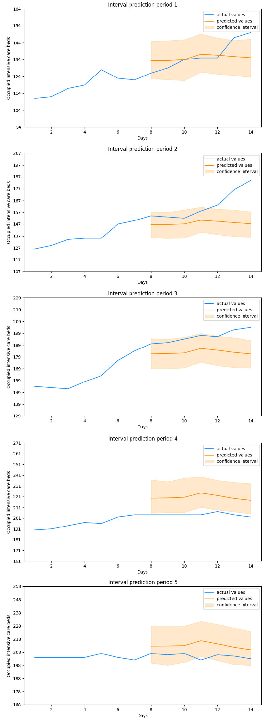
Figure 1.
Bi-LSTM predictions.
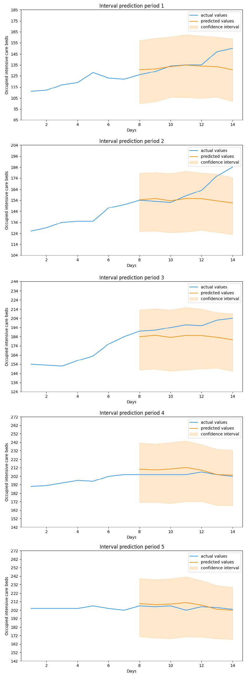
Figure 2.
LSTM predictions.
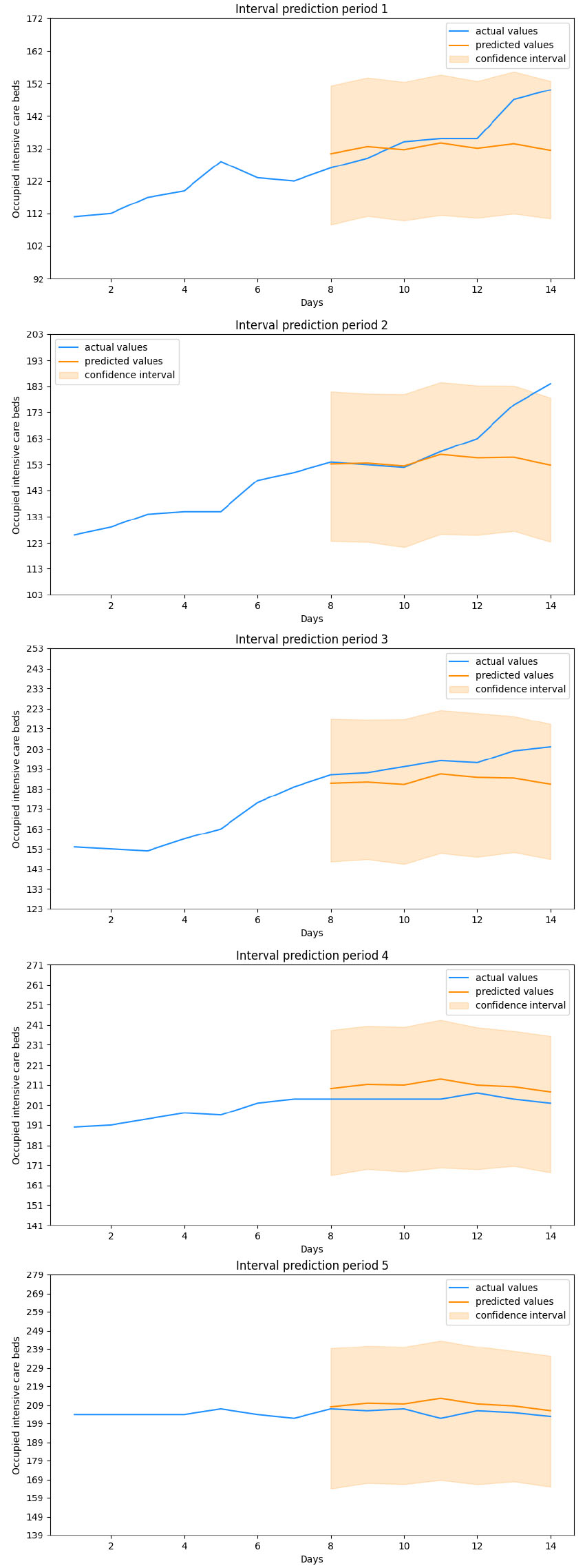
Figure 3.
ARIMA predictions.
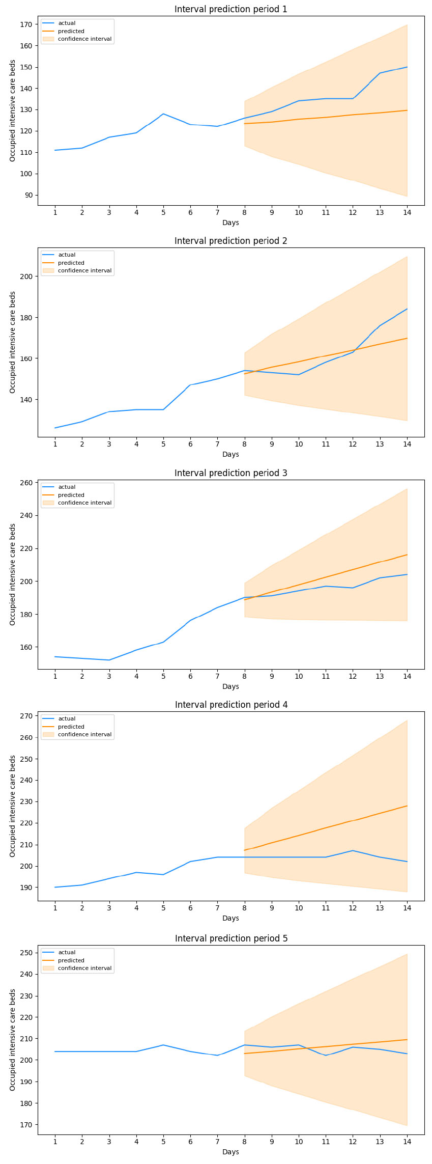
Figure 4.
Ensemble Bi-LSTM predictions.
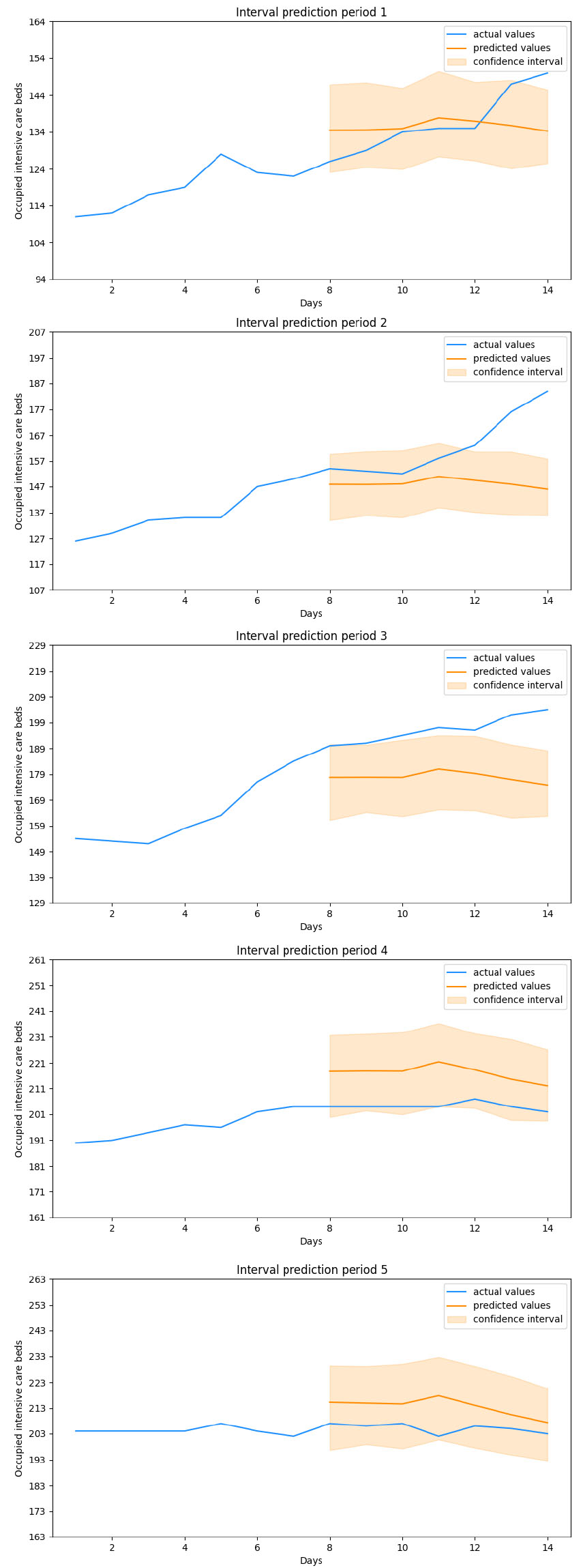
Figure 5.
Ensemble LSTM predictions.
3.Results
The target of the study presented in this paper is to build a forecasting model as accurate as possible, so as to have a powerful tool for evaluating policies aimed at flattening the contagion curve. The dataset has been divided into timesteps of seven days each, passing from a two-dimensional array to a three-dimensional one where the first dimension represents the number of weeks that make up the training set, the second the width of the timestep (that is seven days) while the third the number of variables selected. The selection of the hyperparameters was carried out through trial and error, as well as the number of input days. A schematic of the final configuration is shown the Table 2 [26, 27, 28]. In addition, to ensure greater comparability with the standards in force in the literature, two traditional ensemble models were also developed. These were built by separately training 100 models, respectively of LSTM and Bi-LSTM, whose predictions are then obtained by calculating the average of each individual output week. We can see how both the stochastic and the traditional ensemble have rather similar configurations: both report the same values as regards to Batch Size and Learning Rate, respectively equal to
Table 3
Hyperparameters of architectures for both LSTM and Bi-LSTM ensemble models
| Neurons | Batch size | Learning rate | Optimizer | Activation function | Dropout | |
|---|---|---|---|---|---|---|
| Bi-LSTM | 32 | 1 | 0.001 | Adam | Sigmoid | 0.25 |
Table 4
Value of metrics for the Bi-LSTM model
| Period 1 | Period 2 | Period 3 | Period 4 | Period 5 | |
|---|---|---|---|---|---|
| MAE | 5.942 | 9.91 | 12.345 | 4.315 | 3.004 |
| RMSE | 9.146 | 15.261 | 13.726 | 5.171 | 3.864 |
Table 5
Value of metrics for the LSTM model
| Period 1 | Period 2 | Period 3 | Period 4 | Period 5 | |
|---|---|---|---|---|---|
| MAE | 7.697 | 8.805 | 9.076 | 6.369 | 4.058 |
| RMSE | 8.326 | 14.314 | 10.296 | 6.608 | 4.931 |
Figure 6.
Distribution of metrics for the two architectures of the stochastic ensembles.
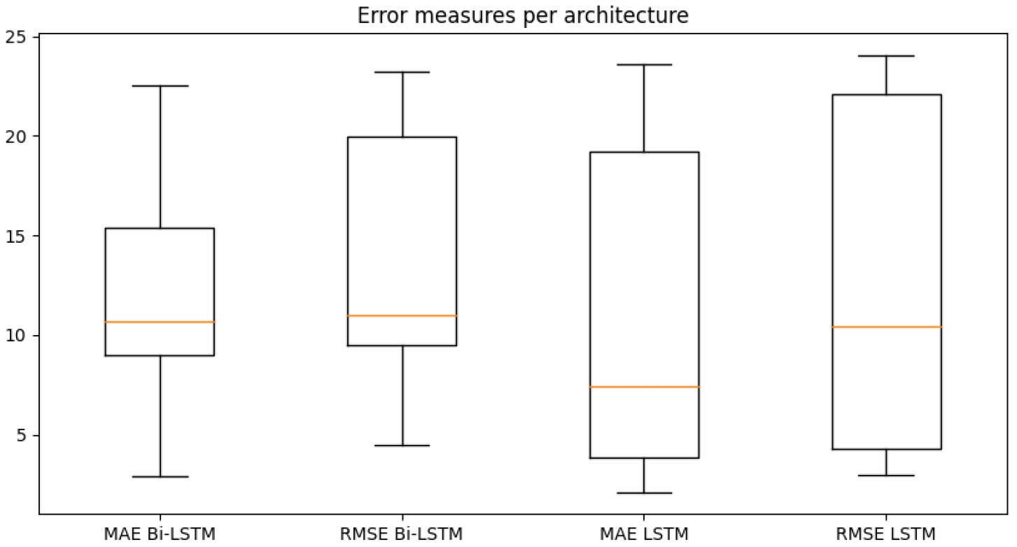
This said, we move on to analyze the performances of the forecast models obtained. The dataset we have adopted runs from March 13, 2020 to January 27, 2021, for a total of 686 days. Among these, 525 days have been used to train the models, 126 consitute the validation set while the remaining 35, that means 5 weeks, have been used for the evaluation. The results obtained from each model over these five evaluation periods have been displayed in Figs 1 to 5. In addition to the values useful for comparing each forecasted week with the one that actually took place, the values assumed by the target variable in the previous seven days have also been shown in the figure. These values represent the period taken as input, together with the other variables, by the Neural Networks. The final evaluation will be conducted on the basis of the overall performances obtained in over 1000 cycles of these predictions while all error metrics refer to a generic cycle among them and where each cycle represents the output of a stochastic ensemble of 1000 Neural Networks. The boxplots built by aggregating these 1000 cycles obtained on the various predicted weeks have been displayed in Fig. 6. Observing Tables 4 and 5, containing the metrics obtained on the five evaluation periods, we note that both stochastic ensembles report rather similar MAE and RMSE values. With reference to periods 1 and 2 there is a large difference between the two metrics, highlighting the presence of infrequent forecast errors but of a significant size. This is confirmed by Figs 1 and 2 depicting the forecasts of the periods just mentioned: in the first plot in fact both architectures correctly capture the evolution of the number of occupied intensive care beds for most of the week in question, except for the last two days where there is a sudden increase in hospitalized patients. The same is true for the second period, where the increase is such that it goes out of the estimated confidence interval. It is worth noting how in both cases this happens in the last estimated days, in fact when the latest available data is further away and therefore where greater uncertainty in the output is expected. In the remaning 3 evaluation periods both architectures achieve a higher level of precision, correctly anticipating what the actual values and any changes in the trend will be, without significant differences between MAE and RMSE. Looking at the boxplot in Fig. 6 we notice how both architectures settle on similar ranges of Mean Absolute Error and Root Mean Squared Error. The LSTM reports a median value of the MAE lower than all the other metrics, which amounted to around 10, at the expense of a higher interquantile range, approximately between 5 and 20, for both measures of error, in fact resulting less stable in forecasts than the Bi-LSTM. However, both stochastic ensembles report values of the distributions of an order of magnitude lower than the target variable, thus confirming the goodness of the forecasts obtained. By comparing the results of the stochastic ensemble with those obtained through a traditional one we observe how the latter stands at higher MAE and RMSE values than the former (Tables 7 and 8). What was previously said about periods 1 and 2 remains valid, where also in this case the sudden increases are not anticipated correctly, while weeks 3, 4 and 5 are characterized by greater precision in forecasting the trend, net of a greater deviation from the real values compared to the previous ensemble. It is also important to note that the confidence intervals themselves in this case are much smaller in width, in fact not providing useful information on the possible evolution of the target variable (Figs 4 and 5). Worth noting is that training a traditional ensemble is significantly more expensive than training a stochastic one, as in the first case it is necessary to repeat the training phase
Table 6
Value of metrics for the ARIMA model
| Period 1 | Period 2 | Period 3 | Period 4 | Period 5 | |
|---|---|---|---|---|---|
| MAE | 10.123 | 5.433 | 6.487 | 13.466 | 3.286 |
| RMSE | 11.905 | 7.039 | 7.628 | 15.288 | 3.679 |
Table 7
Value of metrics for the Bi-LSTM ensemble model
| Period 1 | Period 2 | Period 3 | Period 4 | Period 5 | |
|---|---|---|---|---|---|
| MAE | 6.547 | 14.391 | 18.284 | 12.407 | 7.799 |
| RMSE | 8.381 | 19.058 | 19.283 | 12.645 | 8.402 |
Table 8
Value of metrics for the LSTM ensemble model
| Period 1 | Period 2 | Period 3 | Period 4 | Period 5 | |
|---|---|---|---|---|---|
| MAE | 5.8 | 15.007 | 13.369 | 16.48 | 7.831 |
| RMSE | 7.825 | 18.946 | 14.352 | 16.572 | 8.332 |
Table 9
Value of metrics for the Bi-LSTM model with non-shifted data
| Period 1 | Period 2 | Period 3 | Period 4 | Period 5 | |
|---|---|---|---|---|---|
| MAE | 15.482 | 33.996 | 23.941 | 5.097 | 8.69 |
| RMSE | 18.659 | 36.208 | 24.974 | 5.659 | 9.737 |
Table 10
Value of metrics for the LSTM model with non-shifted data
| Period 1 | Period 2 | Period 3 | Period 4 | Period 5 | |
|---|---|---|---|---|---|
| MAE | 21.67 | 36.227 | 35.01 | 4.914 | 4.118 |
| RMSE | 23.453 | 38.332 | 35.522 | 5.462 | 5.084 |
ARIMA of order (2,2,2) has been developed to serve as a benchmark. Its parameters were estimated according to AIC and BIC while its results are shown in Table 6. We can observe in Table 6 how in this case MAE and RMSE values are generally comparable, and in some cases better, than those obtained with Artificial Neural Networks, except for some spikes where these error measures increase significantly. By visualizing the periods where these increases have been reported, we note how these are characterized by a change in trend for the target time series. On the other hand where MAE and RMSE are low, we note how these are composed by a linear evolution of occupied intensive care beds. This phenomenon is mainly due to the inputs that the Machine Learning model receives. In fact, being based exlusively on the values assumed by the variable in previous timesteps, the output results in a continuation of what was observed before. This implies that when this phenomenon actually happens, the Autoregressive Integrated Moving Average presents excellent metrics, being by construction particularly effective in predicting linear time series. We can see a representation of what just stated in periods 2 and 5, in Fig. 3. In the first case we note how the model, which reports lower MAE and RMSE values compared to both stochastic ensemble architectures, continues the trend it observed in input, projecting it into the forecasting period. This, despite the output of the Neural Networks being more precise in the first 4 days of the week, is ultimately confirmed as more effective in describing the actual growth found in all 7 days of the evaluation period. This is different in the second case, where despite a linear trend, the Bi-LSTM is still more effective, albeit slightly, in terms of error metrics. When it comes to non linear trends however, the ARIMA model utterly fails at the task,not having the piece of information required to anticipate these variations. This is striking in period 4, where a change in trend coinciding with the end of the input data causes the model to completely mistake the evolution of the number of beds occupied in intensive care. This change is instead precisely captured by both Bi-LSTM and LSTM, which report lower Mean Absolute Error and Root Mean Squared Error values and predictions more consistent with real data. The forecasts obtained through ARIMA are therefore not consistent and, in a framework where the objective is to effectively predict the evolution of this type of data, they are almost useless, being unable to forecast trend variations. This result also confirms the validity of the adoption of mobility data, which are confirmed to be extremely useful in order to predict the degree of hospital use.
4.Conclusions
In this paper, the objective was to lay the foundations for the construction of a system based on Deep Learning methodologies to foster predict COVID spread through targeted and preventive measures. Knowing in advance what the likely evolution of the degree of hospital use will be in specfific regions will allow individual jurisdictions to implement containment policies based on this additional information. Assuming with a sufficient degree of certainty a growing trend for occupied ICUs can lead to the application of restrictions on regional mobility which are more severe the more steep the expected increase is. These restrictions would take place a week earlier than what has been done so far, effectively allowing a contraction of their possible duration. The possibility of being able to complement the precise forecasts with an interval estimate also makes the application of tools of this kind much more concrete as it is possible to associate a risk measure to each forecast, as is done for example in the financial and insurance fields[29]. The architecture that best demonstrated that it was able to fulfill this task turned out to be the Bi-LSTM, which surpassed the LSTM in terms of stability of forecasts, despite a similar level of accuracy. A necessary clarification concerns the 21-day shift implemented in the data relating to mobility. Tables 9 and 10 show the values of the forecasts obtained using non-shifted data, confirming how this element is crucial to obtain estimates as precise as possible. In fact, without the 21-day shift of the data relating to mobility, the error metrics assume significantly higher values than the other models, thus not allowing to formulate solid forecasts starting from which to base the implementation of contagion containment policies. A further evolution of what has been presented in this work consists in the forecast of additional variables, such as the total number of hospitalized patients. This variable, combined with the one predicted so far, is the basis of the Italian criterion for classifying the regions according to the level of risk. The implementation of interval estimates makes it possible to calculate the probability that the reference territory (in our case Lazio) changes the level of risk within the following week, thus passing from one Zone to another, calculating the probability that these variables override the thresholds established at national level. With the passage of time the database in our possession to elaborate models of this kind will become more and more extensive, allowing a framework such as the one proposed in the paper to improve its performances over time, guaranteeing more and more accurate forecasts and allowing the management of the pandemic to be increasingly more effective.
References
[1] | World Health Organization 2020, Q&A on coronaviruses (COVID-19). https://www.who.int/emergencies/diseases/novel-coronavirus-2019/question-and-answers-hub/q-a-detail/q-a-coronaviruses. |
[2] | World Health Organization 2021, WHO Coronavirus Disease (COVID-19) Dashboard. https://covid19.who.int. |
[3] | Gopinath G. (2020) . The Great Lockdown: Worst Economic Downturn Since the Great Depression. https://bit.ly/3Eh6JxD. ??? |
[4] | Dacan LI, Huang M, Zhao C, Gong Y, Zhang Y. Construction of 5G intelligent medical service system in novel coronavirus pneumonia prevention and control. Chinese Journal of Emergency Medicine, (2020) , E021-E021. |
[5] | Hossain MS, Muhammad G, Guizani N. Explainable AI and Mass Surveillance System-Based Healthcare Framework to Combat COVID-I9 Like Pandemics, IEEE Network. July/August (2020) ; 34: (4): 126-132. doi: 10.1109/MNET.. |
[6] | Bassi, Pedro RAS, Romis A. A Deep Convolutional Neural Network for COVID-19 Detection Using Chest X-Rays. arXiv preprint arXiv:2005.01578 (2020). |
[7] | Karaca-Mandic P, Sen S, Georgiou A. et al. Association of COVID-19-Related Hospital Use and Overall COVID-19 Mortality in the USA. J GEN INTERN MED, (2020) . doi: 10.1007/s11606-020-06084-7. |
[8] | Cartení A, Luigi Di F, Maria M. How mobility habits influenced the spread of the COVID-19 pandemic: Results from the Italian case study. Science of the Total Environment. (2020) ; 741: : 140489. |
[9] | Shahid F, Aneela Z, Muhammad M. Predictions for COVID-19 with deep learning models of LSTM, GRU and Bi-LSTM. Chaos, Solitons & Fractals. (2020) ; 140: : 110212. |
[10] | Wolpert DH, Macready WG. No free lunch theorems for optimization. IEEE Transactions on Evolutionary Computation. (1997) . 1: (1): 67-82. |
[11] | Mitchell T. Machine Learning. (1997) : 870-877. |
[12] | Hamilton J. (1994) . Time Series Analysis. Princeton University Press. ISBN 9780691042893. |
[13] | Tranmer M, Mark E. Multiple linear regression. The Cathie Marsh Centre for Census and Survey Research (CCSR). (2008) ; 5: (5): 1-5. |
[14] | Graupe D. Principles of artificial neural networks. Vol. 7. World Scientific, (2013) . |
[15] | Siami-Namini S, Tavakoli N, Namin AS. The Performance of LSTM and BiLSTM in Forecasting Time Series, 2019 IEEE International Conference on Big Data (Big Data), (2019) , pp. 3285-3292. doi: 10.1109/BigData47090.2019.9005997. |
[16] | Gers FA, Jürgen S, Fred C. Learning to forget: Continual prediction with LSTM. (1999) ; pp. 850-855. |
[17] | Graves A, Navdeep J, Abdel-Rahman M. Hybrid speech recognition with deep bidirectional LSTM. 2013 IEEE workshop on automatic speech recognition and understanding. IEEE, (2013) . |
[18] | Srivastava N, et al. Dropout: a simple way to prevent neural networks from overfitting. The Journal of Machine Learning Research. (2014) ; 15: (1): 1929-1958. |
[19] | The National Institute for Public Health and the Environment, 2021. 4 in 5 COVID-19 patients in ICU are not vaccinated. https://bit.ly/3lw0Ox9. |
[20] | |
[21] | Dipartimento della Protezione Civile, (2020). Dati Covid Italia [https://github.com/pcm-dpc/COVID-19]. |
[22] | Google LLC “Google COVID-19 Community Mobility Reports”. https://www.google.com/covid19/mobility/Accessed:<data>. |
[23] | https://www.ecdc.europa.eu/en/COVID-19/latest-evidence/transmission. |
[24] | Raudys A, Vaidotas L, Edmundas M. Moving averages for financial data smoothing. International Conference on Information and Software Technologies. |
[25] | Willmott CJ, Matsuura K. Advantages of the mean absolute error (MAE) over the root mean square error (RMSE) in assessing average model performance. Climate Research. 19 December (2005) ; 30: : 79-82. doi: 10.3354/cr030079. |
[26] | arXiv:1803.08375 [cs.NE]. |
[27] | arXiv:1803.09820v2 [cs.LG]. |
[28] | Kingma DP, Jimmy BA. Adam: A method for stochastic optimization. arXiv preprint arXiv:1412.6980 (2014). |
[29] | Solvency II: The Data Challenge, White Paper, 2014, RIMES. |


