
Multilayer perceptron models for the estimation of the attained level of education in the Italian Permanent Census
Abstract
In the Italian Permanent Census, estimates of the attained level of education are derived by the integration of administrative data, 2011 census data, and sample survey data. The result of the integration procedure is the prediction of the attained level of education (ALE) for each single resident. Due to the complexity and heterogeneity of the available information, traditional statistical methods require the construction of different imputation models for different subpopulations, with a considerable effort in terms of human intervention. We study the use of a multilayer perceptron (MLP) model to make the process more automatic, i.e., less costly in terms of human resources, and possibly more accurate in terms of estimates. The MLP model is applied to Istat data referred to an Italian administrative region (Lombardia) in 2018, and the results are compared with those obtained using the official procedure. The study shows that the MLP approach is indeed less demanding in terms of human work needed for data preparation and modeling, yet it leads to estimates characterized by the same level of accuracy as the ones provided by the official procedure.
1.Introduction
The Italian National Institute of Statistics (Istat) is moving towards a register-based production system. The new Italian Census is one of the most important outcomes of this statistical program. The Attained Level of Education (ALE) is one of the output figures provided by the Census. Istat released official estimates of the ALE for the 2018 and 2019 resident population by using predicted values for each unit in the Italian Base Register of Individuals (BRI) [1, 2].
ALE is the result of a multisource approach: it makes use of administrative data, the 2011 Italian (traditional) Census, and sample survey data. Log-linear models are applied to estimate ALE. Due to the complexity and heterogeneity of the available information, this approach requires an expensive initial phase of data analysis and treatment to achieve an accurate prediction. Moreover, different imputation procedures must be combined to deal with sub-populations characterized by different amounts of information.
In the last years, machine learning (ML) techniques have been applied in many contexts (including official statistics, see [3]) with the aim of improving predictions, especially when very large collections of data can be leveraged. The advantage of using such techniques is also in their almost automated application to data. These opportunities motivated the study of ML for the ALE prediction task, with the twofold objective of improving estimation accuracy (given the high amount of available data) and reducing human workload (given the efforts needed for data treatment and sequential usage of complex models in the official procedure).
In recent years, Istat has gained considerable experience in the use of neural networks to extract statistical information from extremely large and unstructured data sets generated by non-traditional sources. In particular, the potentialities of deep-learning models like convolutional neural networks (CNN) have been investigated in [4, 5, 6] for the treatment of images and natural language. In this study, we focus instead on the Multilayer Perceptron model (MLP). Early applications of the MLP model in the field of official statistics can be found in [7, 8, 9]. More recently, MLP and other machine learning techniques have been studied within the HLG-MOS group [10].
In this paper, we compare predictions of the ALE variable resulting from MLP models to the official ones. First, predictions are computed within the same informative setting, i.e., the same preliminary data analysis and the resulting data elaboration (variable selection and treatment) used for the official procedure is used for MLP. The same covariates are used, with the same level of aggregation. The aim of this experiment is to evaluate the capacity of MLP to improve the quality of predictions. In a second experiment, the MLP model is used in its most natural context, that is, the data is fed to the MLP almost without any selection and aggregation. This second study is useful to assess the possibility of making predictions of ALE in a more efficient and automated way.
The paper is structured as follows. Sections 2 and 3 describe the available data and the procedure adopted to produce official ALE estimates. Section 4 introduces the MLP model and its application to our problem. The experimental study and the results are illustrated in Section 5. Some conclusions and future studies are discussed in Section 6.
2.Basic information about the attained level of education in the Italian Census
The BRI is a comprehensive statistical register storing individual data gathered from various data sources. Core variables – such as place and date of birth, gender, and citizenship – are associated to each unit of the register.
For the ALE prediction procedure, data of different kinds are jointly used: administrative data, 2011 traditional Census data, and sample survey data.
• Administrative data. Administrative information on ALE is gathered by making use of the information collected by the Ministry of Education, University and Research (MIUR). MIUR provides information about ALE and course attendance for people entering a study program after 2011 and covers the period from 2011 to t-2 (scholar year t-2/t-1, where t is the reference year of the estimations).
• 2011 Italian Census data. This is the last traditional Census conducted in Italy before the switch to the current ‘Permanent Census’ design. Its data is used for people who have not attended any courses since 2011 and, consequently, are not covered by the available administrative data so far introduced.
• Sample survey data. A sample survey is carried out to gather updated information on variables, hence a direct measurement for ALE at time t for a subset of population (about 5%) is available. We refer to this sample survey as the census survey (CSt).
The three sources of data are characterized by different patterns and amounts of information, that is a different set of variables and different classifications of ALE.
The structure of available information is summarized in Fig. 1. Blue cells indicate that the information is available for the specific subpopulation.
Figure 1.
Structure of available information for mass-imputation of the attained level of education at time t.
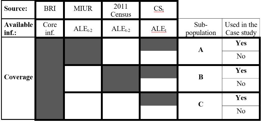
More in detail, core information from BRI is available for all individuals: age, gender, citizenship, marital status, place of birth and place of residence.
The different availability of information on ALE from 2011 to t-2 determines the partition of the population of interest into three subgroups:
A. Subgroup A is composed of all persons with administrative information on ALE from MIUR and is characterized by young people with longitudinal information on school enrollment. B. Subgroup B is composed of persons not in MIUR but interviewed in the 2011 Census, so that the most updated information on ALE dates back to 2011. Since these individuals, mainly adults, did not enroll in any school course registered in MIUR from 2011 to t-2, ALE in 2011 can be considered approximately equal to ALE in time t-2. C. Subgroup C is composed of individuals neither in MIUR nor in 2011 Census. For this group, no direct information on ALE is available. Subgroup C is composed mainly of adults and is mainly characterized by a high percentage of Not Italian people.
In all the subgroups, data on ALE were reclassified according to the 8-item classification adopted by Istat for the purpose of disseminating Permanent Census data. The classification is as follows: 1 – Illiterate, 2 – Literate but no formal educational attainment, 3 – Primary education, 4 – Lower secondary education, 5 – Upper secondary education, 6 – Bachelor’s degree or equivalent level, 7 – Master’s degree or equivalent level, 8 – PhD level.
ALE, at reference time t, is only known for people interviewed in the Census sample, which is a representative subset of the population of interest. For the 95% of population not in the Census sample, ALE has to be estimated. Although ALE is estimated for each individual in the population of interest (micro level), the aim of the prediction procedure is to reproduce the frequency distribution observed in the sample. Hence, the first interest of the prediction is to maximize the distributional accuracy. Nevertheless, since we are dealing with registers that are characterized by individual-level information, predictive accuracy (micro level accuracy) should be evaluated as well.
3.The official estimation procedure based on log-linear models
The official procedure adopted by Istat in production ([2]) is based on log-linear imputation. As stated in Singh (1988) [11], this method generalizes hot-deck imputation by choosing suitable predictors for forming “optimal” imputation classes. In fact, the approach is based on modeling the associations between variables.
The objective of log-linear models is the representation of the interdependence of the variables in the contingency table. In the following we will refer to the case of three categorical variables
A log-linear model is a parameterization of the probabilities
Then, a log-linear model is defined by:
under the constraints
When some of the interaction terms (i.e., the
The idea underlying the approach is that of estimating a model for the prediction of ALE at time t (henceforth
The conditional probabilities
First, a log-linear model is applied to the contingency table obtained by cross-classifying the variables (
It is worthwhile noting that different log-linear models are used within groups A, B and C, mainly because of the different available information. As already remarked, in group A, a log-linear model is estimated by using only administrative data, while for the other groups, log-linear models are estimated by using survey data as well.
For each subpopulation (A, B and C), a step of variable selection was performed to detect the combination of covariates to be included in the model. The best log-linear model is chosen by means of cross-validation. More specifically, log-linear models for each sub-population are built to estimate the following conditional probabilities:
• Subpopulation A: Pr (ALE2018
• Subpopulation B: Pr (ALE2018
• Subpopulation C: Pr (ALE2018
Apr is an auxiliary information on ALE coming from an administrative source and it covers a particular subpopulation of individuals: those who changed their place of residence after 2014. Moreover, it is a self-declared information with a low level of quality, and it comes with a more aggregate classification (4 levels).11 We decided to use ALE from the apr source only in subpopulation C, where we have not any other information on ALE.
Sirea refers to people who were targeted but not surveyed by the 2011 Census and were later detected by post-Census operations carried out in agreement with Italian Municipalities.
An in-depth analysis of the independent variables was necessary to appropriately reclassify the covariates in the model. In particular, suitable age levels were identified by taking into account the structure of the Italian school system and a classification in 14 levels was adopted.22 Citizenship was aggregated into Italian/Not Italian to reduce the number of categories.
4.MLP for the prediction of the attained level of education
As anticipated, this work investigates an alternative approach to the ALE prediction and imputation problem, based on a MLP model.
The MLP (the acronym stands for Multilayer Perceptron) is a supervised machine learning algorithm. When it encompasses more than one hidden layer, the MLP constitutes the simplest example of deep neural network (DNN).
In general, a neural network consists of a network of elementary computing units (artificial neurons) connected according to a specific network topology. In a neural network, each artificial neuron
The architecture of an MLP is organized in layers of neurons. The output of the neurons of the previous layer
Therefore a k-th layer neuron returns an output vector
where
Figure 2.
Example of MLP.
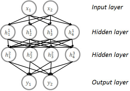
In the Fig. 2 we show an example of MLP with two neurons for the input layer, two neurons for the output layer, and 2 hidden layers with four neurons.
The output of an MLP is a composition of the outputs returned by each layer and realizes a nonlinear mapping between the input and output vectors.
According to the universal approximation theorem [13] and subsequent extensions, any mapping between an input vector X and an output vector Y is arbitrarily approximated by an MLP with a sufficiently large number of neurons or a sufficiently deep number of layers.
The algorithm with which the network is trained according to a dataset of examples is the backpropagation algorithm [14].
Given a task, e.g. classification or regression, and a dataset of examples of a mapping ({Xi, Ti}), in general the loss function represents the distance between the mapping performed by the network {Xi, Yi} and the mapping provided in the dataset. The backpropagation is an iterative algorithm that aims to find, in the space of the weights of a neural network, the minimum configuration of the loss function. A loss-function typically used for a classification task is the cross-entropy defined as:
During each iteration of the backpropagation algorithm, the weights are updated by calculating the gradient of the loss function:
The algorithm terminates when it achieves the best performance on external datasets (validation set).
In our approach we use this neural network architecture for its well-known ability to find, after a training phase, a good approximation of the relationship between the input variables and the distribution of the output variable [15].
In order to predict the ALE of each resident unit in BRI, first a MLP is trained, then, analogously to log-linear models, a random extraction of ALE values from the estimated ALE distribution is performed, conditional to observed covariates. Of course, this reduces prediction accuracy but improves the distributional accuracy, which is our main goal.
Our approach aims to be as general as possible, therefore:
• We train a single neural network, unlike the official procedure, where different models are built, according to the variables available for each of the three profiles.
• We encode the MLP input variables with a one-hot encoding that transforms a categorical variable with C modalities into a binary C-dimensional vector. In this representation, the missing value of a variable is encoded as any other modality of the variable.
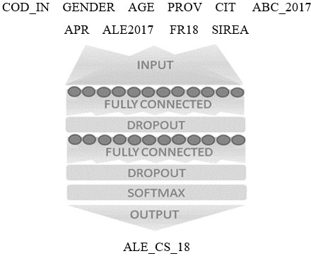
To train the MLP, we employ the cross-entropy as loss function to be minimized. The cross-entropy is a measure of the distance between the distribution of the output variable and the distribution of the target variable. The architecture of the network is shown in Fig. 3: it has two hidden layers of 128 neurons each, and an output layer with 8 neurons (one per modality of the target variable). To limit the risk of over-fitting in the learning phase, two dropout layers have been interposed. The best configuration of some hyper-parameters (number of hidden neurons, dropout probability, learning-rate) was explored through a suitable grid-search.
Figure 3.
Architecture of the implemented MLP model.
For each record of the dataset, the model generates a probability distribution on the 8 ALE items. In a conventional ML approach, the imputed value would be the modal value of the distribution. However, in our case study, an important goal is to best reproduce the distribution of the ALE variable in the population of interest. Therefore, as already mentioned, to increase the distributional accuracy, for each record we impute an ALE item that is randomly extracted from the probability distribution of the corresponding pattern of covariates.
For our case study, we use a Linux server with Ubuntu 16.04.5 LTS operating system, deployed on the Azure cloud platform and equipped with a Tesla V100-PCIE-16GB GPU. The GPU is not strictly necessary but reduces the runtime to train the model.
The training phase of our MLP model lasts about one hour. The runtime mainly depends on three factors. The first factor is the complexity of the model: our MLP has about 27,000 free parameters (the neural network weights); the second factor is the number of iterations (epochs) performed by the optimization algorithm: we set it to 500. The third factor entails the way the training set was built: we adopted a k-fold validation approach and generated a dataset of 312,813 trials (this will be better explained in paragraph).
5.Experimental study
The comparison of MLP with the official imputation model is carried out on the Italian region Lombardia and the subset of population for which the target variable is available (see last column of Fig. 1). The target variable is the self-declared ALE in the 2018 sample census, referring to the year 2018, which corresponds approximately to 5% of total population of interest.
Table 1
Variables in the dataset used in the three log-linear models and MLP approach
| Id | Name | Description | Log-linear | MLP | MLP without pre-processing | ||
| A | B | C | |||||
| 1 | COD_IND | Record id | |||||
| 2 | GENDER | Gender | 1 | 1 | 1 | 1 | |
| 3 | AGE_CLASS | Age classified into 14 levels | 1 | 1 | 1 | 1 | |
| 4 | AGE | Age in years | 1 | ||||
| 5 | BIRTH_MU | Municipality of birth | 1 | ||||
| 6 | BIRTH_CO | Country of birth | 1 | ||||
| 7 | MUN | Municipality of residence | 1 | ||||
| 8 | PROV | Province of residence | 1 | 1 | 1 | ||
| 9 | CIT_CLASS | Citizenship (Italian/Not Italian) | 1 | 1 | 1 | 1 | |
| 10 | CIT | Country of citizenship | 1 | ||||
| 11 | ABC_2017 | Subpopulation (A, B C) | 1 | ||||
| 12 | APR | ALE from APR classified into 4 levels | 1 | 1 | 1 | ||
| 13 | ALE2017 | 2017 ALE (combination of Administrative and 2011 Census) | 1 | 1 | 1 | 1 | |
| 14 | FR18_CLASS | Aggregated type of school and year of attendance in 2017/2018 | 1 | 1 | |||
| 15 | FR18 | Type of school and year of attendance in 2017/2018 | 1 | ||||
| 16 | SIREA | Resident in Italy in 2011 not caught by the 2011 Census | 1 | 1 | 1 | ||
| 17 | ALE_CS18 | 2018 ALE from 2018 Census Survey | Target variable | ||||
Note that people with complete longitudinal information on course attendance from administrative sources (part of subpopulation A in Fig. 1) are excluded from this experimentation, as the knowledge of their schooling history, until scholar year 2017/2018, would make the ALE 2018 prediction task too easy. Further studies will be devoted to this subset of units.
The dataset for the experimentation consists of 312,813 people residents in Lombardia in 2018 with no missing data on ALE 2018 (target variable). This is the sum of sub-populations A-Yes, B-Yes and C-Yes in Fig. 1.
A first experiment is carried out by using the MLP with the same covariates selected for log-linear models. The goal is to minimize confounding factors, therefore allowing for a neat comparison of results in terms of statistical accuracy. In a second experiment, data provided to MLP are not pre-processed: all the variables in the dataset enter the MLP algorithm without any selection or reclassification. In particular, the variables age and citizenship are not aggregated into classes and the variables relating to the type of school attended are used as they are presented from administrative sources, without any type of aggregation. The variables relating to the place of residence and place of birth are also included. Moreover, the information on the data source of the three subpopulations is not considered and the flag variable (ABC_2017) which identifies the three subgroups A, B and C, is not introduced. This second experiment is clearly meant to study the possibility of using a more automated approach for the prediction of the ALE variable in large-scale production settings.
The variables used in the different experiments are described in Table 1.
The results of estimates obtained with MLP are compared with the ones obtained with the official procedure. Quality measures are concerned with predictive accuracy of each unit and accuracy of estimated aggregates (quantities obtained by aggregating the unit predictions). The first measure is generally the one analyzed in ML approaches, while the second is usually taken into account in National Statistical Institutes when evaluating the quality of an estimation procedure. We note that it is not necessarily true that a method with the best predictive accuracy is also the best in terms of accuracy of aggregates. This issue has been extensively investigated in the Machine Learning literature, see for instance [16, 17]. Since the ALE distribution will be published by gender, age classes and citizenship, it is important to evaluate the distributional accuracy in these specific subpopulations. The aggregates considered in this study refer to the main figures that are officially disseminated by Istat. In particular, we report results for the ALE distribution by citizenship.
Accuracy is calculated using the k-fold approach with k
(1) the model is estimated on the training set, consisting of 4 of the 5 subgroups,
(2) the results are applied on the test set, composed of the remaining subgroup,
(3) accuracy is calculated only on the test set as the difference between estimated ALE 2018 and the observed ALE 2018.
Tasks 1–3 are repeated 5 times so to reconstruct the entire data set. The same approach is used for both ML and log-linear models so that results can be compared.
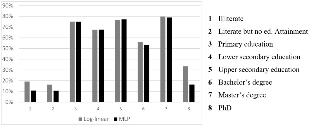
Figure 4.
Item accuracy: Log-linear vs MLP estimation (test set 2, run 1).
After the implementation of this approach each individual (in each k-fold) has two probability distribution on the 8 ALE items, estimated using ML and log-linear models. The imputation process consists of extracting a random value from the probability distribution. The same imputation process is repeated 100 times to consider the model variability and the resulting indicators are averaged over those repetitions.
5.1Accuracy results
Table 2 shows the micro-level predictive accuracy attained by the log-linear and MLP approaches in the first experiment. For each method and k-fold, the proportions of units whose predicted ALE equals the observed (i.e. true) value are reported as percentages.
Table 2
Micro-level accuracy in the 5 test sets averaged over 100 runs: Log-linear vs MLP estimation (percentage values)
| K-fold | Log-linear | MLP |
|---|---|---|
| 1 | 72.154 | 72.052 |
| 2 | 72.140 | 72.182 |
| 3 | 72.269 | 72.267 |
| 4 | 72.097 | 72.236 |
| 5 | 72.081 | 71.935 |
| Mean | 72.148 | 72.134 |
| Standard deviation | 0.066 | 0.124 |
The results of the MLP are very similar to those originated from log-linear models: the average predictive accuracy, computed over the 5 folds, are respectively equal to 72.13% and 72.15%; and the standard deviation is quite small in both cases (0,07% vs 0,12%).
Predictive accuracy can also be calculated for each item; specifically, item accuracy is calculated as the number of individuals for which ALE has been correctly estimated, with respect to the total number of individuals with a certain observed ALE:
Item
In Fig. 4, the item accuracy obtained by the log-linear and MLP approaches are depicted as side-by-side bar charts. We notice that, in general, the most inaccurate estimates are concentrated on some categories (1, 2, 8) and that those categories are the ones where the MLP behaves worse. It is interesting to note that those categories are the ones with fewer observations and presumably this is the reason behind the differences highlighted. The results reported in Fig. 4 concern only one k-fold and one run (specifically the first run on the second fold); the item accuracy computed using the imputations from other runs and other folds shows similar results.
To evaluate the performance of the imputation procedures at macro-level, the estimated frequency distribution of ALE in 2018 (
A possible synthetic measure (AD) is given by the average of the absolute values of the differences between the frequencies of ALE categories as computed from estimated and sampled data. A second measure (RD) can be used to assess the overall effect of relative discrepancies. In detail
where
In addition, the Kullback-Leibler divergence is computed:
It measures the divergence of the distribution
Results of the AD, RD and D
Table 3
Macro-level accuracy (AD, RD, D
| K-fold | Log-linear | MLP | ||||
|---|---|---|---|---|---|---|
| AD | RD | D | AD | RD | D | |
| 1 | 0.060 | 2.664 | 0.007 | 0.081 | 2.987 | 0.011 |
| 2 | 0.079 | 2.614 | 0.008 | 0.071 | 3.941 | 0.019 |
| 3 | 0.086 | 2.242 | 0.009 | 0.132 | 4.499 | 0.027 |
| 4 | 0.113 | 4.405 | 0.026 | 0.105 | 3.263 | 0.014 |
| 5 | 0.076 | 2.707 | 0.009 | 0.118 | 4.254 | 0.023 |
| Mean | 0.083 | 2.926 | 0.012 | 0.101 | 3.789 | 0.018 |
| Standard | 0.017 | 0.757 | 0.007 | 0.023 | 0.577 | 0.006 |
| deviation | ||||||
The frequency distribution of ALE 2018 predicted using the MLP is slightly worse than the one obtained using log-linear models. The predictions differ from the observed data by 0.08 and 0.10 percentage points on average on each item for log-linear and MLP, respectively. In relative terms the MLP approach performs a little worse: the average relative differences are 2.93% and 3.79% for the log-linear and MLP, respectively. The Kullblack-Leibler divergence confirms that the ALE distribution obtained from log-linear models is closer to the 2018 census sample distribution than the distribution obtained from MLP. The standard deviations of the accuracy measures show that both models are stable.
Since the ALE distribution will be published yearly by Istat along with some other variables such as gender, age classes, citizenship, it is important to evaluate the distributional accuracy of the estimated ALE in specific subpopulations defined by those variables. Looking at ALE 2018 distribution by citizenship and comparing the two estimation approaches with the target variable distribution (Table 4) we notice that largest differences are related to the subpopulation of ‘not Italian’. This subpopulation is much smaller than the Italian one, consisting of about 27 thousand individuals (less than 9% of total population analyzed), and less information is available for it.
Table 4
Relative differences between Estimated and target ALE 2018 distribution by citizenship: Log-linear vs MLP estimation (test set 2 averaged over 100 runs)
| ALE in 2018 | Italian | Not Italian | ||
|---|---|---|---|---|
| Log- linear (Drel | MLP (Drel | Log- linear (Drel | MLP (Drel | |
| Illiterate | ||||
| Literate but no ed. Att. | 14.833 | |||
| Primary education | 0.689 | 2.326 | 14.659 | |
| Lower secondary ed. | 0.511 | 0.112 | ||
| Upper secondary ed. | 0.136 | |||
| Bachelor’s degree | 0.010 | 28.771 | 15.388 | |
| Master’s degree | 0.073 | 0.387 | 2.711 | |
| PhD | 7.762 | 13.667 | 124.933 | |
| Mean (RD) | 1.897 | 4.438 | 8.564 | 24.373 |
The relative differences between estimated and target distributions are larger for Not Italian people than for Italian people and are concentrated in the extreme and less frequent categories. As it can be noticed, larger differences are evident for the MLP: the differences between the estimated and target frequencies are almost always larger for the MLP than for the log-linear models.
5.2MLP analysis without pre-processing
As far as efficiency is concerned, we study the application of MLP with raw (not pre-treated) data. We remind that for the official procedure, first variables need to be carefully selected, then they also need to be smartly aggregated to avoid estimation issues arising from sparse cells in contingency tables.
In the MLP without variable pre-treatment, the input variables are more detailed and not aggregated into classes. In the specific case, age enters in years, place of residence enters with the detail of the Municipality of residence (and not only the province), citizenship is specified as country of citizenship (instead of the dummy coding Italian/Not Italian), and school attendance is more detailed (without grouping by type of school). Moreover, in addition to the variables used in the log-linear model, other information is introduced as covariates: place of birth and marital status (see Table 1).
Micro and macro level accuracy of imputed ALE 2018 using MLP without variable selection or pre-treatment (MLP all-in) are reported in Table 5.
Table 5
Micro and macro-level accuracy (AD, RD, D
| Log-linear | MLP all-in | |||||||
| Fold | Micro accuracy (%) | Macro accuracy | Micro accuracy (%) | Macro accuracy | ||||
| AD | RD | D | AD | RD | D | |||
| 1 | 72.154 | 0.060 | 2.664 | 0.007 | 73.490 | 0.115 | 2.458 | 0.012 |
| 2 | 72.140 | 0.079 | 2.614 | 0.008 | 73.594 | 0.124 | 2.484 | 0.014 |
| 3 | 72.269 | 0.086 | 2.242 | 0.009 | 73.670 | 0.103 | 2.886 | 0.013 |
| 4 | 72.097 | 0.113 | 4.405 | 0.026 | 73.545 | 0.149 | 3.997 | 0.024 |
| 5 | 72.081 | 0.076 | 2.707 | 0.009 | 73.448 | 0.093 | 2.587 | 0.010 |
| Mean | 72.148 | 0.083 | 2.926 | 0.012 | 73.549 | 0.117 | 2.882 | 0.015 |
| St. dev. | 0.066 | 0.017 | 0.757 | 0.007 | 0.078 | 0.019 | 0.578 | 0.005 |
Table 6
Relative differences between Estimated and target ALE 2018 distribution by citizenship: Log-linear vs MLP vs MLP All-in estimation (test set 2 averaged over 100 runs)
| ALE in 2018 | Italian | Not italian | ||||
|---|---|---|---|---|---|---|
| Log- linear (Drel | MLP (Drel | MLP All-in (Drel | Log- linea (Drel | MLP (Drel | MLP All-in (Drel | |
| Illiterate | 0.324 | |||||
| Literate but no ed. Att. | 14.833 | 11.515 | ||||
| Primary education | 0.689 | 1.824 | 2.326 | 14.659 | 8.510 | |
| Lower secondary ed. | 0.511 | 0.112 | ||||
| Upper secondary ed. | 0.136 | |||||
| Bachelor’s degree | 0.010 | 1.255 | 28.771 | 15.388 | 17.418 | |
| Master’s degree | 0.073 | 0.387 | 2.711 | |||
| PhD | 7.762 | 13.667 | 124.933 | 80.133 | ||
| Mean (RD) | 1.897 | 4.438 | 1.961 | 8.564 | 24.373 | 15.490 |
Note that in MLP using raw data, micro accuracy is slightly improved: the predictive accuracy reaches 73.55% and the standard deviation computed on the 5 folds decreases from 0.12 to 0.08. But the most important result is that MLP has greatly improved its performance in terms of distributional accuracy, in fact MLP and log-linear models now perform similarly.
However, low performances remain for some subpopulations, such as Not Italian people (Table 6).
6.Conclusions
In Istat, the increasing use of administrative data poses the need to investigate new methods that can efficiently handle large amounts of heterogeneous data and still lead to output statistics of satisfactory accuracy. The statistical procedures used so far in the statistical production system generally require preliminary tasks of data analysis and data treatment that are very expensive in terms of resources. Moreover, even when surveys are repeated in time, these preliminary tasks must be performed for each new round (although perhaps with less effort), at least for confirming the data treatment adopted in previous rounds. Machine learning techniques can be useful to alleviate this problem since they are naturally applied in an automated way. A study on real data is performed to analyze whether a MLP model can improve the official procedure adopted in the Italian Permanent Census for the prediction of the attained level of education of each Italian resident. The evaluation focuses on two quality aspects: accuracy of predictions (and of estimated aggregates computed by directly using the predictions) and efficiency of the procedure. The efficiency assessment is primarily concerned with the automation of the process, which means that resources spent for data analysis and preparation can be minimized. Results are encouraging especially concerning the efficiency. In fact, we do not notice an improvement in terms of accuracy, but the same level of quality is reached by using raw data, that is without resorting to expensive data pre-treatment steps.
There are still some open problems to deal with for the application of the MLP approach to the production of official ALE statistics. The first is concerned with the presence of sampling weights. In this application, survey data are used without taking into account sampling weights. The role of sampling weights is to make the sample representative of the whole population, thereby leading to unbiased estimates. While techniques to incorporate sampling weights in classical statistical models are well developed in the literature, the same cannot be said for machine learning models. Further studies will be devoted to shed light on this important issue.
Another important question is concerned with the evaluation of uncertainty of estimates obtained by using the MLP approach. When official statistics are disseminated, National Statistical Institutes (NSI) must provide a measure of their accuracy. This is a fundamental piece of information that increases the credibility of NSIs. Common measures of accuracy (under the assumption of negligible bias) are estimated coefficients of variation and confidence intervals. MLP outcomes are evaluated by accuracy measures as well, but this mostly happens in contexts that are very different from official statistics, both in terms of data and goals. In fact, machine learning techniques are mostly aimed at micro-level prediction, rather than at estimation of population parameters. This aspect as well deserves further analysis.
Notes
1 Apr 4 levels of classification: 1 – Up to primary education; 2 – Lower secondary education; 3 – Secondary and short cycle tertiary education; 4 – Tertiary and post tertiary education.
2 Age levels: 0–8; 9–10; 11; 12–13; 14–17; 18; 19; 20–22; 23–25; 26–28; 29–39; 40–49; 50–69; 70-max.
References
[1] | Di Zio M, Di Cecco D, Di Laurea D, Filippini R, Massoli P, Rocchetti G. Mass imputation of the attained level of education in the Italian System of Registers. Workshop on Statistical Data Editing; 18–20 September (2018) ; Neuchâtel, Switzerland. |
[2] | Di Zio M, Filippini R, Rocchetti G. An imputation procedure for the Italian attained level of education in the register of individuals based on administrative and survey data. Rivista di Statistica Ufficiale. (2019) ; 2–3: , 143–174. |
[3] | Yung W, Karkimaa J, Scannapieco M, Barcarolli G, Zardetto D, Sanchez JAR, Barteld B, Buelens B, Burger J. The Use of Machine Learning in Official Statistics. UNECE Machine Learning Team report. (2018) . UNECE site: https://bit.ly/mlforofficialstats. |
[4] | Bernasconi E, De Fausti F, Pugliese F, Scannapieco M, Zardetto D. Automatic extraction of land cover statistics from satellite imagery by deep learning. Statistical Journal of the IAOS. (2022) ; 38: (1). |
[5] | De Fausti F, Pugliese F, Zardetto D. Automated Land Cover Maps from Satellite Imagery by Deep Learning. In: Pearson. Book of short Papers – SIS 2020. (2020) . pp. 242–247. ISBN 9788891910776. |
[6] | De Fausti F, Pugliese F, Zardetto D. Towards automated website classification by Deep Learning. Rivista di Statistica Ufficiale. (2020) ; 3: , 9–50. ISSN 1828-1982. |
[7] | Nordbotten S. Editing statistical records by neural networks. Journal of Official Statistics. (1995) ; 11: (4), 391–411. |
[8] | Nordbotten S. Neural network imputation applied to the Norwegian 1990 Population Census data. Journal of Official Statistics. (1996) ; 12: (4), 385–401. |
[9] | Charlton J. Editorial: Evaluating Automatic Edit and Imputation Methods, and the EUREDIT Project. Journal of the Royal Statistical Society. Series A (Statistics in Society). (2004) ; 167: (2), 199–207. |
[10] | HLG-MOS site: https://statswiki.unece.org/display/ML/HLG-MOS+Machine+Learning+Project. |
[11] | Singh AC. Log-linear imputation. Methodology Branch Working Paper Statistics Canada. (1988) ; 88–29. |
[12] | Agresti A. An introduction to categorical data analysis. John Wiley & Sons, (2018) . |
[13] | Pinkus A. Approximation theory of the MLP model in neural networks. Acta Numerica. (1999) Jan; 8: , 143–195. |
[14] | Rumelhart D, Hinton G, Williams R. Learning representations by back-propagating errors. Nature. (1986) a; 323: (6088), 533–536. |
[15] | Cybenko G. Approximation by superpositions of a sigmoidal function. Mathematics of Control, Signals and Systems. (1989) ; 2: (4), 303–314. |
[16] | Forman G. Quantifying counts and costs via classification. Data Mining and Knowledge Discovery. (2008) ; 17: (2), 164–206. |
[17] | González P, Castaño A, Chawla NV, Coz JJD. A review on quantification learning. ACM Computing Surveys (CSUR). (2017) ; 50: (5), 1–40. HLG-MOS site: https://statswiki.unece.org/display/ML/HLG-MOS+Machine+Learning+Project. |


