
Influence of technologies on the growth rate of GDP from agriculture: A case study of sustaining economic growth of the agriculture sector in Bihar
Abstract
The influence of agricultural technologies on the growth of agricultural value-added based on time series data of Bihar (India) over the period 1990–2016 has been examined in this paper. The technological progress appears to be a major determinant of boosting the potential productivity of land and affecting positively the economic growth. The results indicated that there are significant and certain benefits from the utilization of a system of technological innovations including mechanization, renewed capital stocks, as well as transfer of new knowledge to farmers’ and permanent cropping practices. Farming practices involving crop rotation, multi-cropping, and agro forestry are recommended to sustain agricultural sustainability since they seem to be economically viable and environmentally friendly. It was found that technological innovations pertaining to soil conditions, irrigation systems and chemical fertilizers might be beneficial to agricultural production growth in the long-term when they are managed in accordance with soil characteristics and in a balanced way. The results also showed that the labour force, the forest area, the amount of credits to agriculture, and the amount of energy consumed to power irrigation are likely to be insignificant to boost directly the growth of agricultural value-added. Thus, it is recommended that Bihar makes a large scale investment in agricultural capital and carry on renewal at opportune moments so as to keep steady the positive trend of the agricultural growth over the years. The investment may be in terms of mechanized technologies, supporting infrastructure and appropriating the knowledge relating to their management; and adopting new farming technologies and practices involving crop rotation, multi-cropping and agro-forestry so as to sustain the growth of agricultural value added.
1.Introduction
The world is facing a key challenge to grow food sustainably to meet the demand of the growing population without degrading the natural resources base and the United Nations advocates the adoption of resource-conserving technologies and sustainable production practices in the agricultural field. In recent years, agricultural production increasingly depends on science and technology advances, farm infrastructures, fertilizers and pesticides use, planting structures for crops, water management and policy for agriculture development. Different input factors have different influences on agricultural production. For instance, while the Integrated Pest Management (IPM) seeks to use pesticides when other options are ineffective [1, 6], the Integrated Nutrients Management (INM) recommends to balance both organic and inorganic fertilizers [5] for a green production. Actually, owing to some serious concerns, sustaining the agricultural production growth and yields requires nowadays the application of Fertilizer Best Management Practice [10] as a key technological innovation, in the regions that are highly dependent on agriculture and have substantial employment and income arising from subsistence farming.
Several classifications of technological innovations have been made to differentiate policies or modeling. One categorization distinguishes between technologies that are embodied (such as machines, fertilizers, and seeds) and those that are disembodied (e.g., integrated pest management schemes, a set of new practices) [4]. Another categorization distinguishes between neutral and non-neutral technologies: Harrod-neutral if the technology is labour-augmenting (i.e. helps labour); Solow-neutral if the technology is capital-augmenting. The technological progress function developed by Nicholas [9] measures technological progress as the rate of growth of labour productivity. So, a technological change may cause the production-possibility frontier to shift outward, allowing economic growth. In this context, Wang and Zhou [18], after measuring the contribution rate of scientific and technological progress, suggested that the sector of construction and industry should rely on technological progress so as to improve the international competitiveness and realize the sustainable development goal. Except for scientific and technological progress, a number of researches [11, 13, 16] turned the attention of government and practitioners towards agricultural technologies and practices concerns, and then, diverse mathematical models such as Cobb-Douglas production function, and Solow remaining value model [7, 12, 14, 15], have been used to measure their contribution to agricultural production in the short and long terms. Kumar and Yadav [8] found that the yield response of grains (rice and wheat intercropped) to a direct Nitrogen (N) fertilizer supply would decline over a long period, and in contrast, the application of Phosphorus (P) and Potassium (K) would increase the grains yields. Moreover, a balanced dose of N-P-K is required to maintain durable soil fertility and raise grains yields. Obviously, the increase on crop yields also related to many other factors. Some researchers basically drew attention upon the impact of human capital investments and fixed capital stock investments on agricultural gross domestic product and some, investigated on the impact of irrigated land [2].
2.Purpose of the study
This paper proposes to study the influence of technologies in value addition that contribute towards compilation of the gross domestic product from agriculture especially in the backward regions with prominent subsistence farming to facilitate potential changes in the income structure. This background is made to examine the case of Bihar, one of the prominent states of India with 10.2% population, currently lying at the lower rung of the industrial development index (with 1.5 percent share in number of factories; 0.34 percent share in fixed capital; 0.58 percent share in working capital; 0.84 percent share in persons engaged; and 0.84 percent share in value of output to All India) as the contribution of the industrial sector to the state’s GSDP stands at 19.0 percent in 2015-16, compared to the national average of 31.3 percent. It is highly dependent on agriculture, with substantial employment and income arising from subsistence farming. It is important to investigate how the range of agricultural technologies like mechanization, chemical technology, management practices and policies relating to cropping, as well as other agricultural infrastructures, could improve value addition to the gross domestic product besides the common factors of production (capital stock, labour force, land area). The main issues investigated are: How are agricultural technologies linked to the agricultural production growth and what association of agricultural technologies should be deployed for sustaining the growth of the agricultural gross domestic production in Bihar.
This study depends on the Cobb-Douglas (C-D) production function to determine the influence of agricultural technologies on the growth of agricultural value-added in Bihar (India) over the period 1990–2016. Then, an analysis is made of the response of agricultural value-added growth over time following technological innovations or shocks, and the corresponding findings are put forward.
Table 1
Variable definitions and data sources
| Variable | Definition | Sources |
|---|---|---|
| AGRIVA | Agricultural value-added (Rs million, value price 2011) | DES, Bihar, 2017 |
| NETK | Net capital stocks value (Rs million, value price 2011) | Author estimate, 2017 |
| MACHI | Number of machines (tractors, harvesters, threshers) used | DES, Bihar, 2017 |
| CREDI | Amount of credits to agriculture (Rs million, value price 2011) | NABARD, 2017 |
| ENERG | Amount of energy used to power irrigation, in Million Kwh | Govt. of Bihar, 2017 |
| LABOR | Number of workers in agriculture sector | DES, Bihar, 2017 |
| ALAND | Land for arable land and permanent crops (area in hectare) | DES, Bihar, 2017 |
| FORES | Land for planted and naturally regenerated forest (area in hectare) | DES, Bihar, 2017 |
| IRRIG | Land equipped for irrigation (area in hectare) | DES, Bihar, 2017 |
| FERTIL | Chemical fertilizers (nitrogen, phosphorus and potassium) consumed (quantity in tons) | DES, Bihar, 2017 |
3.Modeling and data description
3.1Theoretical modeling
The mathematical equation estimated in this study, based on Cobb-Douglas (C-D) production function, may be written as:
(1)
where
It may be demonstrated that the
(2)
Hence,
(3)
(4)
Where
(5)
where
3.2Data
The dataset supporting the conclusions of this article comprises of one endogeneous variable Agricultural value added and nine exogeneous variables:
1. Net capital stock;
2. Number of machines (tractors, harvesters, threshers) used;
3. Amount of credit to agriculture;
4. Energy used to power irrigation;
5. Number of workers in the agriculture sector;
6. Area of arable land and permanent crops;
7. Area on planted and naturally regenerated forest;
8. Area equipped for irrigation;
9. Amount of chemical fertilizers consumed.
These variables comprise part of the official statistics compiled regularly by the various government agencies and were obtained from the Directorate of Economics and Statistics, Bihar and other related departments of the Bihar government/government of India. The modeling adopted is based on annual time series data for 27 years (1990–2016) on these ten variables, obtained from these sources. Table 1 provides variable definitions and data sources.
The data were examined for stationary of time trend with the null hypothesis of the Augmented Dickey-Fuller
H
And thereafter the data were processed through suitably developed R-Programming.
Table 2
Descriptive statistics of variables
| LAGRIVA | LNETK | LMACHI | LCREDI | LENERG | LLABOR | LALAND | LFORES | LIRRIG | LFERTIL | |||||||||||
|---|---|---|---|---|---|---|---|---|---|---|---|---|---|---|---|---|---|---|---|---|
| Mean | 13 | .2247 | 13 | .2103 | 5 | .2640 | 8 | .3390 | 3 | .9335 | 7 | .3359 | 7 | .8468 | 8 | .5074 | 2 | .7103 | 9 | .1964 |
| Median | 13 | .2671 | 13 | .2306 | 5 | .2204 | 8 | .9860 | 3 | .9411 | 7 | .3524 | 7 | .9338 | 8 | .4992 | 2 | .6391 | 9 | .7549 |
| Maximum | 13 | .7350 | 13 | .3351 | 5 | .4553 | 10 | .4571 | 3 | .9411 | 7 | .5011 | 8 | .0709 | 8 | .6656 | 3 | .1355 | 10 | .9455 |
| Minimum | 12 | .5952 | 13 | .0656 | 5 | .0434 | 0 | .0000 | 3 | .9240 | 7 | .0475 | 7 | .4501 | 8 | .3689 | 2 | .3026 | 3 | .4965 |
| Std.Dev | 0 | .3452 | 0 | .1067 | 0 | .1264 | 2 | .1330 | 0 | .0086 | 0 | .1285 | 0 | .2152 | 0 | .0902 | 0 | .3711 | 1 | .8895 |
| Skewness | 0 | .3092 | 0 | .1577 | 0 | .0303 | 2 | .3479 | 0 | .2236 | 0 | .5237 | 0 | .8283 | 0 | .1196 | 0 | .0985 | 1 | .6399 |
| Kurtosis | 1 | .8479 | 1 | .2548 | 1 | .8422 | 9 | .6442 | 1 | .0500 | 2 | .3029 | 2 | .2204 | 1 | .8701 | 1 | .1836 | 4 | .8064 |
| Jarque-Bera | 1 | .9236 | 3 | .5383 | 1 | .5122 | 74 | .4700 | 4 | .5028 | 1 | .7808 | 3 | .7710 | 1 | .5008 | 3 | .7556 | 15 | .7729 |
| Probability | 0 | .3822 | 0 | .1705 | 0 | .4695 | 0 | .0000 | 0 | .1053 | 0 | .4105 | 0 | .1518 | 0 | .4729 | 0 | .1529 | 0 | .0004 |
| Sum | 357 | .068 | 356 | .679 | 142 | .128 | 225 | .152 | 106 | .204 | 198 | .070 | 211 | .863 | 229 | .699 | 73 | .178 | 248 | .304 |
| Sum.Sq.Dev. | 3 | .0989 | 0 | .2960 | 0 | .4154 | 118 | .2907 | 0 | .0019 | 0 | .4291 | 1 | .2037 | 0 | .2113 | 3 | .5804 | 92 | .8298 |
| Observations | 27 | 27 | 27 | 27 | 27 | 27 | 27 | 27 | 27 | 27 | ||||||||||
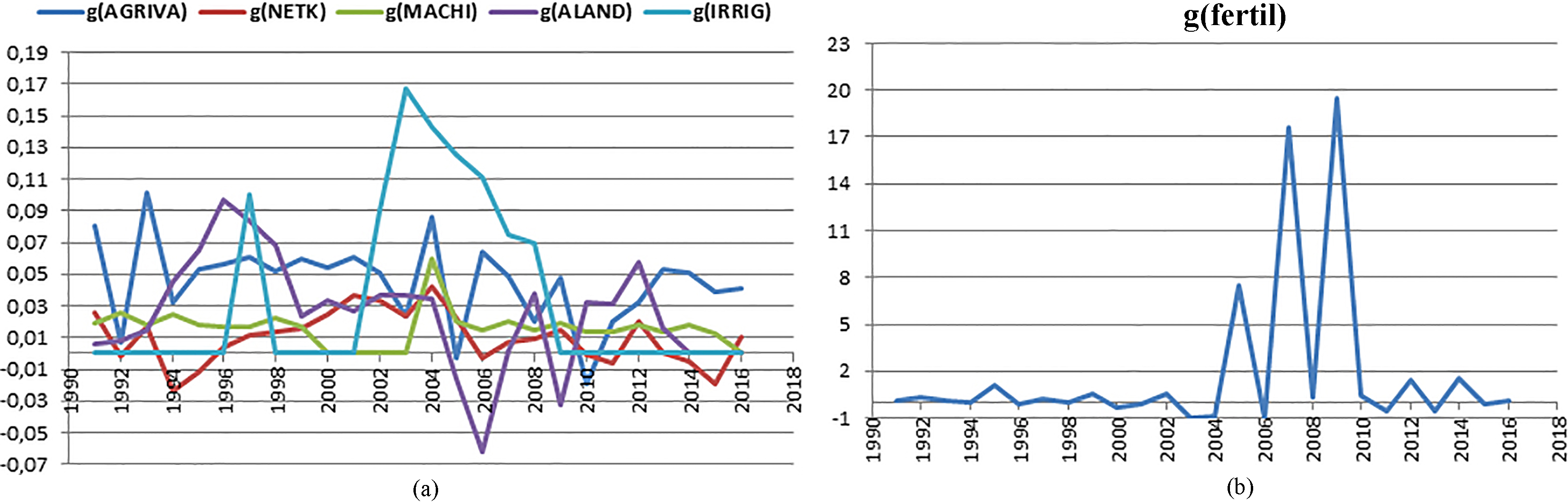
Figure 1.
a. Growth rate of AGRIVA; NETK; MACHI; ALAND; and IRRIG, b. Growth rate of FERTIL.
4.Descriptive statistics on variables
Data processed through the suitably developed R-Progamming is presented in Table 2. Table 2 provides a description of variables (in logarithm) in terms of central tendency and dispersion. Over the period of study, the average value-added is about Rs 1322 billion, almost identical to the average value of net capital stocks. The discrepancy between the maximum and minimum values of each variable is likely to be insignificant except for FERTIL as it is shown in Fig. 1b. The statistics show with exception of IRRIG and FORES of which the mean values are greater than the Median values, that all other variables are negatively skewed. In addition, it is found that all variables show a leptokurtic tendency given that their kurtosis coefficients are positive. The statistics also inform about a normal distribution regarding all variables except CREDI and FERTIL.
Figure 1a and b describe the trend of the annual growth rate of variables and indicates that the evolvement of variables has not been steady over the study period. The trends depict serious fluctuations of the growth rate of agricultural technologies and as a result, an unstable growth rate of agricultural value-added. In 2005 and 2010 (Fig. 1a), the growth of agricultural value-added was negative, showing a certain drop in the value-added with a slight severity in 2010. The highest growth rate is about 16.5% (2003) and attained by IRRIG whereas the lowest growth rate is about
Figure 1a shows trends of annual growth rates of agricultural value-added, net capital stocks, machinery, arable land and permanent crops, and area equipped for irrigation (1990–2016).
Figure 1b shows trend of annual growth rate of chemical fertilizers (1990–2016).
Table 3
The augmented Dickey-Fuller unit-root test on variables: results
| Variables | Unit-root test in | ADF test statistic | Test critical values | Integration order |
|---|---|---|---|---|
| LAGRIVA | First difference, including intercept | I(1) | ||
| LNETK | First difference, without intercept nor trend | I(1) | ||
| LMACHI | First difference, including intercept | I(1) | ||
| LCREDI | First difference, without intercept nor trend | I(1) | ||
| LENERG | First difference, without intercept nor trend | I(1) | ||
| LLABOR | First difference, including intercept and trend | I(1) | ||
| LALAND | First difference, without intercept nor trend | I(1) | ||
| LFORES | First difference, including intercept | I(1) | ||
| LIRRIG | Second difference, without intercept nor trend | I(2) | ||
| LFERTIL | First difference, without intercept nor trend | I(1) |
Figure 2.
a and b show relationship between agricultural value added and machinery and area equipped for irrigation. c and d show relationship between agricultural value added and fertilizers and arable land and permanent crops.
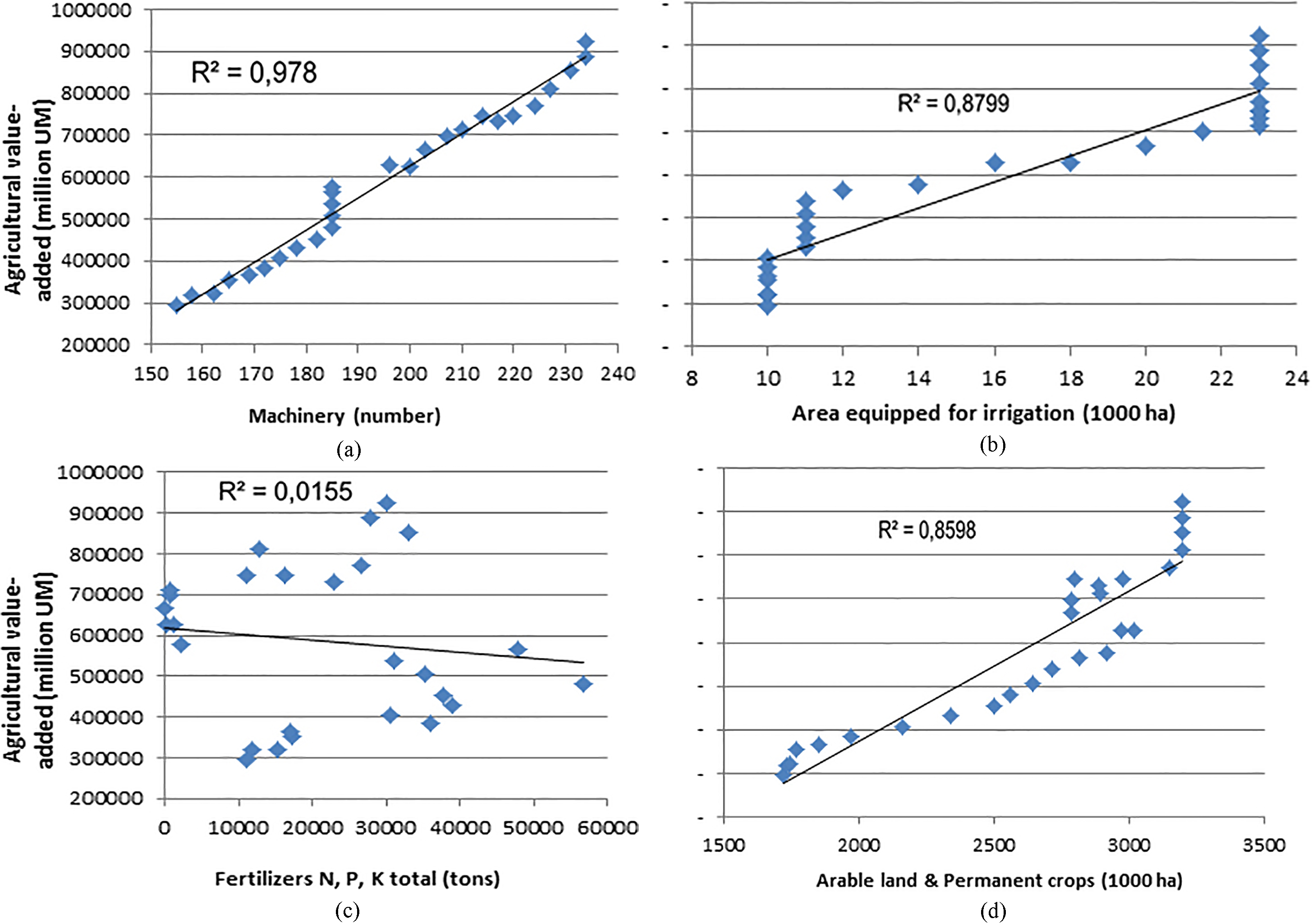
Figure 2 describes the linear relation between agricultural technologies and agricultural value-added. It indicates that the number of machines used, the number of hectares equipped for irrigation, and the number of hectares for arable land and permanent crops, are greatly related to the growth of agricultural value-added. Therefore, a linear model might explain correctly the relationship between the underlying variables, which may help to boost the growth of agricultural production in association with these underlying technologies. However, the agricultural gross domestic product is likely to be inexplicable by the amount of chemical fertilizers in terms of linear relation in this study.
Figure 2a shows relationship between machinery and agricultural value-added (1990–2016) and Fig. 2b relationship between area equipped for irrigation and agricultural value-added (1990–2016).
Finally Fig. 2c shows relationship between chemical fertilizers and agricultural value-added (1990–2016), whereas Fig. 2d shows relationship between arable land and permanent crops area and agricultural value-added (1990–2016).
5.Empirical results and discussion
5.1Unit-root test on variables
It may be mentioned that log of the data was taken to avoid exponential trending before differencing. The Augmented Dickey-Fuller (ADF) tests in Table 3 show that the null hypothesis for each variable does have a unit-root at a level that cannot be rejected. While the endogeneous variable agricultural value added (LAGRIVA) and five exogeneous variables: net capital stock (LNETK); number of machines (LMACHI); amount of credit to agriculture (LCREDI); land equipped for irrigation (LIRRIG); and chemical fertilizer consumed (LFERTIL) could not be rejected even at the 1% level – the rest of the four exogeneous variables could not be rejected at the 5% level. Then, all these variables were converted into first difference or second difference (LIRRIG) for further analysis.
Table 4
Estimation of the growth of agricultural value-added
| Sample $ | ||||
|---|---|---|---|---|
| Variable | Coefficient | S.E. | ||
| Constant | 5374 | 34. | 48855 | |
| YEAR | 0. | 041686 | 0. | 011901 |
| LNETK | 0. | 586066 | 0. | 203309 |
| LMACHI | 0. | 886031 | 0. | 352736 |
| LCREDI | 0. | 003155 | 0. | 004138 |
| LENERG | 0. | 958764 | 1. | 200274 |
| LLABOR | 029977 | 0. | 488572 | |
| LALAND | 0. | 383954 | 0. | 094556 |
| LFORES | 1. | 766482 | 1. | 259222 |
| LIRRIG | 268012 | 0. | 082152 | |
| LFERTIL | 004634 | 0. | 002418 | |
| Dum1 | 0. | 079432 | 0. | 015338 |
| Dum2 | 045332 | 0. | 016504 | |
| AR(3) | 688183 | 0. | 275643 | |
| Adjusted R | 0. | 997 | ||
| F-statistic | 800. | 48 | ||
| Durbin-Watson stat (DW) | 2. | 358 | ||
Sample $: 1990–2016 (
5.2Estimation of parameters α i
Based on Eq. (4), the growth of agricultural value-added is estimated as shown in Table 4, by running the relevant econometric model containing an autoregressive component. Moreover, two dummy variables (Dum1, Dum2) were introduced in order to capture respectively the impact of sectorial development policy and strategy and natural phenomena (e.g. flooding, precipitations). These variables influenced the growth of agricultural value-added since the null hypothesis that their coefficients are equal to zero cannot be accepted.
The regression model performs well, predicting 99% of the specified equation correctly. F-statistic was calculated to establish the causality between the growth of agricultural value-added and its determinant factors. All the diagnostic tests on the residuals coming from the long-run model estimation (serial correlation, heteroscedasticity, normality) are desirable.
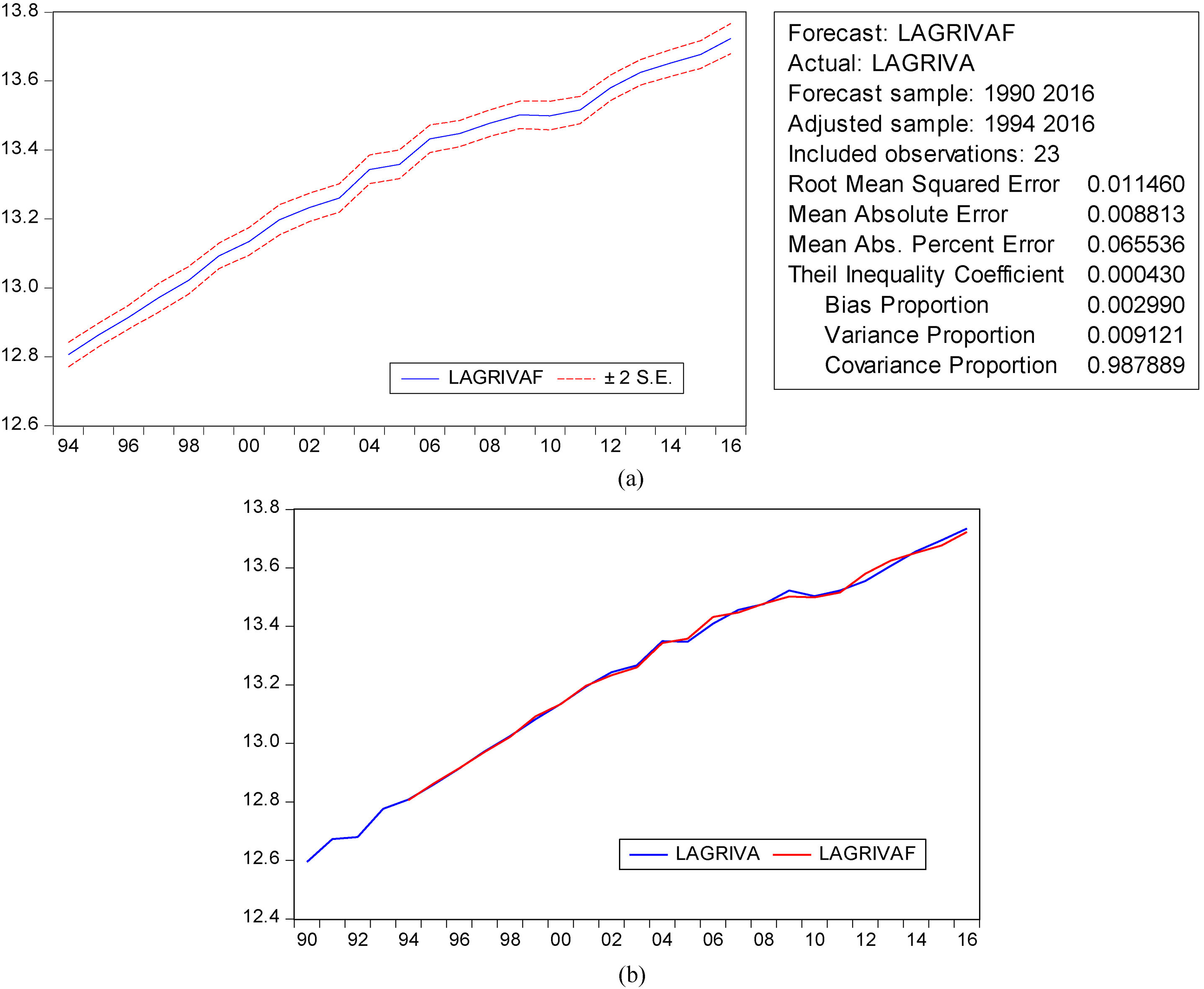
5.3Prediction of the growth of agricultural value-added
This section analyzes the gap between the forecasted value (LAGRIVAF) and the value of LAGRIVA estimated in Section 5.2 named actual value. The objective is to determine the goodness of fit of the estimated regression model. Figure 3a pertaining to the forecasted value indicates that the Root Mean Squared Error is set to only 1.146% and the curve of LAGRIVAF is passing through 95% the confidence interval. The Theil Inequality Coefficient shows a perfect fit as well. As a result, we may conclude that the forecasted and actual LAGRIVA are moving closely, and then, the predictive power of the estimated regression model is quite satisfactory. This can be observed in Fig. 3b where both LAGRIVA and LAGRIVAF are plotted together.
Table 5
Impulse response of agricultural value-added (1–10 years)
| PERIOD | LAGRIVA | LNETK | LMACHI | LALAND | LIRRIG | LFERTIL |
|---|---|---|---|---|---|---|
| 1 | 0.016548 | 0.000000 | 0.000000 | 0.000000 | 0.000000 | 0.000000 |
| 2 | 0.000938 | 0.001880 | 0.004575 | 0.003364 | 0.003025 | 0.006375 |
| 3 | 0.009523 | 0.000622 | 0.008313 | 0.003506 | ||
| 4 | 0.005766 | 0.001267 | 0.011745 | 0.010891 | 0.002663 | |
| 5 | 0.000604 | 0.003451 | 0.007465 | 0.016807 | 0.003770 | |
| 6 | 0.003461 | 0.005264 | 0.008238 | 0.018609 | 0.002293 | |
| 7 | 0.000132 | 0.005264 | 0.008238 | 0.016867 | 0.001389 | |
| 8 | 0.002821 | 0.002423 | 0.004726 | 0.012513 | 0.001753 | |
| 9 | 0.004001 | 0.006643 | 0.009692 | |||
| 10 | 0.003092 | 0.006889 | 0.009398 | 0.001047 |
Figure 3.
a: Trend of forecasted growth of agricultural value-added (1990–2016). b: Gap between actual and forecasted growth of agricultural value-added (1990–2016). Source: Suitably developed programmes in R-Language.
6.Impulse response of agricultural production growth
This section provides information on how agricultural value-added will further be reacting in the short, medium and long terms to a positive innovation or shock to an agricultural technology. Analysis and the graphical presentation of the shocks to the net capital stock (LNETK), number of machines (LMACHI), number of hectares of arable land and permanent crops (LALAND), number of hectares equipped for irrigation (LIRRIG), and number of tons for chemical fertilizer (LFERTIL) and their effect on the agricultural value added function was done using Cholesky (d.f. Adjusted) innovation with suitably developed R-Programming. The response is presented in Table 5.
Figure 4.
Impulse response of agricultural value-added growth (1–10 years).
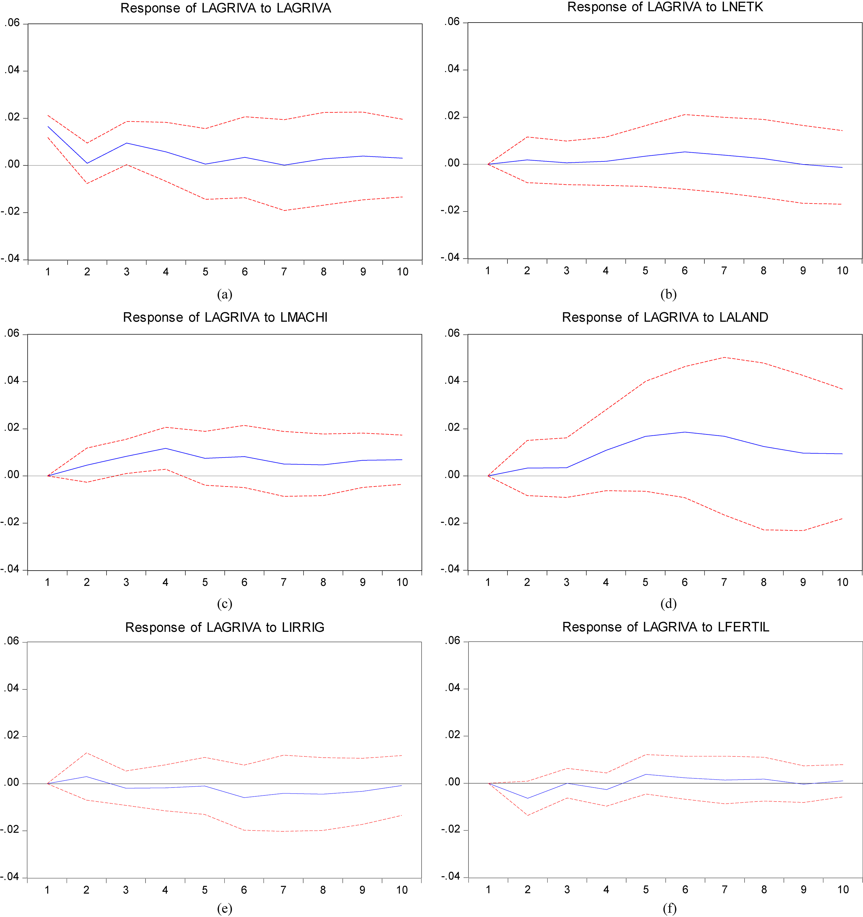
It is found that today’s innovation to machinery (LMACHI) and arable land and permanent crops area (LALAND) in Bihar is continuously positive for the ten years (depicted in Fig. 4c and d) and may be affecting positively and steadily the growth of agricultural value-added within 10 years (long term). Therefore, the goal of sustainable agriculture should rely on mechanized technologies and farming practices involving multi-cropping and agro-forestry.
The growth of agricultural value-added in Bihar responding positively to a net capital stocks (LNETK) are positive for the first 8 years, but turning negative in the ninth and tenth years (depicted in Fig. 4b) which implies that in the short and medium terms (1–8 years) it may be positively affecting the growth of agricultural value added, but it may be declining and turning into negative effects after 8 years (long term). Accordingly, it may be inferred that capital investments should be reinforced or renewed at opportune moments so as to keep steady the positive trend of the agricultural economic growth over the years.
The growth of agricultural value-added in Bihar may be responding negatively within 10 years further to a shock to irrigation technologies (LIRRIG) as indicated by Fig. 4e. However, this negative response may be reversed after 10 years, indicating that once farmers do appropriate soil characteristics and other sub-factors relating to irrigation technologies management, these latter might impact positively the production growth. Meanwhile, the positive response of LAGRIVA to LFERTIL’s impulsion (Fig. 4f) is likely to dominate the negative effect in the long term (after 4 years). However, the impulse response is plainly negative in the short term. For sustainable agricultural goal, it may be suggested that these chemical technologies should be applied in a balanced ratio.
Furthermore, it is found that the output growth may be reacting successfully within 10 years when a shock is directly put to the overall production system (Fig. 4a).
7.Conclusions and recommendations
This article examined the influence of agricultural technologies on the growth of agricultural value-added based on time series data (1990–2016) for Bihar which leads to the following conclusion.
Technological progress appears to be a major determinant of boosting the potential productivity of land and affecting positively the growth of agricultural value added in Bihar through new farming devices and practices like multi-cropping, agro-forestry, new varieties of seeds, and new resources management. Investment in capital stock has shown a contribution of 13% in the present study (Table 2) and farmers have increased the agricultural value added by 0.59% with 1% increase in the capital stock, provided supporting infrastructure such as road is ensured. It has also been found that the contribution of the number machines in increasing the agricultural value added is 32%, so it is destined to capture the importance of agricultural mechanization (labour saving technology) – which might foster the drop of some production inputs like labour and the saving of work time. The growth of agricultural value-added in Bihar responding positively to a net capital stocks are positive for the first 8 years, but turning negative in the ninth and tenth years (depicted in Fig. 4b) which implies that in the short and medium terms (1–8 years) may be positively affecting the growth of agricultural value added, but it may be declining and turning into a negative effect after 8 years (long term). Accordingly, it may be inferred that capital investments should be reinforced or renewed at opportune moment so as to keep steady the positive trend of the agricultural economic growth over the years. It is found that today’s innovation to machinery and arable land and permanent crops area in Bihar is continuously positive for the ten years (depicted in Fig. 4c and d) and may be affecting positively and steadily the growth of agricultural value-added within 10 years (long term). Therefore, the goal of sustainable agriculture should rely on mechanized technologies and farming practices involving multi-cropping and agro-forestry.
Permanent cropping may be encouraged as the contribution of the factor ALAND is established approximately to 21% in Bihar. The number of hectares arranged for arable land and permanent crops is significant and influences positively the growth of the agricultural gross domestic product. Since this variable includes sustainable farming practices like multi-cropping, crop rotation and agro-forestry, the probability that it is positively related to the sustainable agricultural growth and as such the practice of agro-forestry on a farmland might be quite beneficial to the green agricultural revolution with some staple crops namely rice, corn and wheat.
Both the number of hectares equipped for irrigation and the amount of chemical fertilizers appear to be negatively related to the growth of agricultural value-added. Many aspects must be considered in analyzing this outcome given that sometimes, the positive effects generated by applying land-conserving technologies may not compensate their negative externalities. Currently, the pursuit of the agricultural sustainable development goal in Bihar (India) not only relies on chemical fertilizers, but also considers their mixture with organic manure. None of variables LABOR, FORES, CREDI, and ENERG are found to be significant determinants of agricultural value-added growth. In other words, the underlying variables are not likely to foster increasing directly the agricultural value-added.
Conclusions derived from this study leads to following recommendations:
1. Bihar may take a large scale investment in agricultural capital as this factor appeared to be greatly related to the growth of agricultural production value.
2. The capital investments should be reinforced or renewed at opportune moments so as to keep steady the positive trend of the agricultural economic growth over the years.
3. The capital investment on agricultural mechanization may lead to a drop in labour, which may be imparted skill for new farming devices and resources management practices.
4. The labour force strengthened with new knowledge and modern practices may have a significant role in multi-cropping, agro-forestry, adoption of new varieties of seeds, and increasing area for arable land and permanent crops, which could influences positively the growth of the agricultural gross domestic product.
5. The credit received by the farmers do not impact the growth of agricultural value added. It needs to be examined whether the amount of credits is too insignificant to generate increasing return to scale or the amount vanish due to an imperfect management.
6. The contribution of the sub-sector of forest seems to be negligible. However, out of their economic role, forests may be recognized an environmental role like carbon dioxide sinks (positive externalities).
References
[1] | Bale J.S., van Lenteren J.C., Bigler F. ((2008) ). Biological control and sustainable food production. Phil. Trans. R. Soc. B. 363: , 761-776. doi: 10.1098/rstb.2007.2182. |
[2] | Chao W., Sun J. Contribution of Agricultural Production Factors Inputs to Agricultural Economic Growth in Xinjiang. Guizhou Agricultural Sciences, 2013–11. |
[3] | Dorward A., et al. ((2004) ). A policy agenda for pro-poor agricultural growth. World Development. 32: , 73-89. |
[4] | David S., David Z. ((2000) ). The Agricultural Innovation Process: Research and Technology Adoption in a Changing Agricultural Sector (For the Handbook of Agricultural Economics). California, 103. |
[5] | Goulding K., et al. ((2008) ). Optimizing nutrient management for farm systems. Phil. Trans. R. Soc. 363: , 667-680. |
[6] | Hassanali A., et al. ((2008) ). Integrated pest management: the push-pull approach for controlling insect pests and weeds of cereals, and its potential for other agricultural systems including animal husbandry. Philosophical Transactions of the Royal Society B: Biological Sciences. 363: (1491), 611. |
[7] | Khan S.U. ((2006) ). Macro determinants of total factor productivity in pakistan. State Bank of Pakistan Research Bulletin. 2: (2), 384-401. |
[8] | Kumar A., Yaday D.S. ((2008) ). Long-Term Effects of Fertilizers on the Soil Fertility and Productivity of a Rice-Wheat System. July 2008. |
[9] | Nicholas K. ((1957) ). A model of economic growth. The Economic Journal. 67: (268), 591-624. |
[10] | Roberts T.L. ((2007) ). In Fertilizer Best Management Practices: General Principles, Strategy for their Adoption, and Voluntary Initiatives vs. Regulations. IFA International Workshop on Fertilizer Best Management Practices. 7–9 March 2007. Brussels, Belgium. pp. 29-32. |
[11] | Saha S. ((2012) ). Productivity and openness in indian economy. Journal of Applied Economics and Business Research. 2: (2), 91-102. |
[12] | Sarel M., Robinson D.J. ((1997) ). Growth and Productivity in ASEAN Countries, IMF Working Paper No.97/97. |
[13] | Sivasubramonian S. ((2004) ). The Sources of Economic Growth in india, 1950–51 to 1999–2000. OUP, New Delhi. |
[14] | Solow R.M. ((1956) ). A contribution to the theory of economic growth. Quarterly Journal of Economics. 70: (1), 65-94. |
[15] | Suman P., et al. ((2016) ). Modelling impacts of chemical fertilizer on agricultural production: a case study on Hooghly district, West Bengal, India. Model Earth System Environment. 2: , 180. |
[16] | Viramani A. ((2004) ). Sources of India’s Economic Growth: trends in Total factor productivity. ICRIER Working Paper No.131. |
[17] | Wang J., Yu Y. ((2011) ). Determining contribution rate of agricultural technology progress with CD production functions. Energy Procedia. 5: , 2346-2351. |
[18] | Wang K.T., Zhou M.J. ((2006) ). An Analysis of Technological Progress Contribution to the Economic Growth in Construction Industry of China. Construction & design for project. |
[19] | Zhao K.J. ((2011) ). Research on scientific and technological progress contribution to economic growth in Shandong Province, Journal of Shandong Jianzhu University. |
[20] | Zhu J., Cui D. ((2011) ). Estimating and forecasting the contribution rate of agricultural scientific and technological progress based on Solow residual method. In Proceedings of the 8th International Conference on Innovation & Management, Nov.30–Dec.2, pp. 281-287. |
Appendices
Appendix
| Year | AGRIVA | NETK | MACHI | CREDI | ENERG | LABOR | ALAND | FORES | IRRIG | FERTIL |
|---|---|---|---|---|---|---|---|---|---|---|
| (million MU) | (million MU) | (number) | (million MU) | (terajoule) | (1000 people) | (1000 ha) | (1000 ha) | (1000 ha) | (tons) | |
| 1990 | 295124.295927 | 472395.94 | 155 | 0 | 50.6044 | 1150 | 1720 | 5761 | 10 | 11003 |
| 1991 | 319006.425994 | 484616.04 | 158 | 11000 | 50.6044 | 1212 | 1730 | 5700 | 10 | 11817 |
| 1992 | 321140.374332 | 483696.95 | 162 | 430 | 50.6044 | 1279 | 1745 | 5621 | 10 | 15325 |
| 1993 | 353662.038410 | 492080.38 | 165 | 5510 | 50.6044 | 1311 | 1770 | 5551 | 10 | 17238 |
| 1994 | 365271.834742 | 480494.11 | 169 | 480 | 50.6044 | 1343 | 1850 | 5500 | 10 | 17055 |
| 1995 | 384536.97777 | 474901.39 | 172 | 600 | 50.6044 | 1371 | 1970 | 5411 | 10 | 3600 |
| 1996 | 406061.474990 | 476539.81 | 175 | 4530 | 50.6044 | 1395 | 2160 | 5341 | 10 | 30681 |
| 1997 | 430761.675887 | 481940.03 | 178 | 1000 | 50.6044 | 1416 | 2340 | 5300 | 11 | 38968 |
| 1998 | 453363.510806 | 488456.63 | 182 | 1000 | 50.6044 | 1435 | 2500 | 5201 | 11 | 3707 |
| 1999 | 480487.40523 | 495999.45 | 185 | 4134 | 50.6044 | 1455 | 2560 | 5131 | 11 | 56700 |
| 2000 | 506602.247692 | 508337.62 | 185 | 6100 | 50.6044 | 1478 | 2645 | 5061 | 11 | 35200 |
| 2001 | 537490.587059 | 526739.46 | 185 | 6600 | 50.6044 | 1504 | 2715 | 5011 | 11 | 31100 |
| 2002 | 564584.390067 | 544460.60 | 185 | 8110 | 51.4724 | 1531 | 2815 | 4961 | 12 | 47841 |
| 2003 | 577843.419442 | 557177.98 | 185 | 8900 | 51.4724 | 1561 | 2917 | 4911 | 14 | 2126 |
| 2004 | 627617.213824 | 580780.26 | 196 | 7990 | 51.4724 | 1587 | 3017 | 4861 | 16 | 145 |
| 2005 | 626195.000000 | 593481.70 | 200 | 8702 | 51.4724 | 1613 | 2970 | 4811 | 18 | 1226 |
| 2006 | 666418.585965 | 591628.97 | 203 | 6800 | 51.4724 | 1638 | 2785 | 4761 | 20 | 33 |
| 2007 | 698638.387536 | 595822.53 | 207 | 7300 | 51.4724 | 1663 | 2790 | 4711 | 21.5 | 614 |
| 2008 | 712719.778561 | 601192.06 | 210 | 9604 | 51.4724 | 1685 | 2895 | 4661 | 23 | 801 |
| 2009 | 746373.120555 | 609896.21 | 214 | 16770 | 51.4724 | 1705 | 2800 | 4611 | 23 | 16360 |
| 2010 | 731925.343952 | 609674.30 | 217 | 16770 | 51.4724 | 1723 | 2890 | 4561 | 23 | 22826 |
| 2011 | 746607.953106 | 605811.64 | 220 | 24562 | 51.4724 | 1740 | 2980 | 4511 | 23 | 11100 |
| 2012 | 770937.201984 | 618180.79 | 224 | 17170 | 51.4724 | 1755 | 3150 | 4461 | 23 | 26745 |
| 2013 | 811935.972543 | 618514.88 | 2271 | 17861 | 51.4724 | 1769 | 3200 | 4411 | 23 | 12903 |
| 2014 | 853461.901496 | 615280.64 | 231 | 18550 | 51.4724 | 1782 | 3200 | 4361 | 23 | 32954 |
| 2015 | 886550.215097 | 603621.64 | 234 | 34792 | 51.4724 | 1795 | 3200 | 4311 | 23 | 27924 |
| 2016 | 922621.648800 | 610097.86 | 234 | 34792 | 51.4724 | 1807 | 3200 | 4311 | 23 | 301298 |


