
Incremental schema integration for data wrangling via knowledge graphs
Abstract
Virtual data integration is the current approach to go for data wrangling in data-driven decision-making. In this paper, we focus on automating schema integration, which extracts a homogenised representation of the data source schemata and integrates them into a global schema to enable virtual data integration. Schema integration requires a set of well-known constructs: the data source schemata and wrappers, a global integrated schema and the mappings between them. Based on them, virtual data integration systems enable fast and on-demand data exploration via query rewriting. Unfortunately, the generation of such constructs is currently performed in a largely manual manner, hindering its feasibility in real scenarios. This becomes aggravated when dealing with heterogeneous and evolving data sources. To overcome these issues, we propose a fully-fledged semi-automatic and incremental approach grounded on knowledge graphs to generate the required schema integration constructs in four main steps: bootstrapping, schema matching, schema integration, and generation of system-specific constructs. We also present
1.Introduction
Big data presents a novel opportunity for data-driven decision-making and modern organizations acknowledge its relevance. Consequently, it is transforming every sector of the global economy and science, and it has been identified as a key factor for growth and well-being in modern societies.11,22 With an increasingly large and heterogeneous number of data sources available, it is, however, unclear how to derive value from them [21]. It is, thus, commonplace for any data science project to begin with a data wrangling phase, which entails iteratively exploring heterogeneous data sources to enable exploratory analysis [33]. Let us consider the WISCENTD project33 of the World Health Organization (WHO) as an exemplary data science project deeply transforming a traditional organization into a data-driven one. The main goal of this project is to build a system for managing the extraction, storage, and integrated processing of data coming from a variety of data sources related to a group of 21 neglected tropical diseases with diverse and multidimensional natures. For each of these diseases, the data exchange flows are not well-defined and drug distributors, pharmacies, health ministries, NGOs, researchers and WHO analysts generate a wealth of data that is ingested into WISCENTD (specifically, in its Data Lake platform) with different formats and schema. Most of these data have been generated by third parties and the WHO data scientists are often unaware of their schema, which hinders their capacity to conduct comprehensive data analysis. In this context, data wrangling via virtual data integration is nowadays a popular first step toward understanding the available data sources [32]. Oppositely to physical data integration, where data are warehoused in a fixed target schema, virtual data integration systems keep data in their original sources, build an intermediate infrastructure to provide virtual data integration and provide means to retrieve data at query time [26]. Thus, allowing fast and on-demand data exploration in settings that require fresh data. It is however reported that data scientists spend up to 80% of their time in the manual effort of implementing such data integration pipeline, which is a complex and error-prone process that generates a high-entry barrier [34,47] for non-IT people. As a result, most current efforts are ad-hoc for a given project and do not generalize. From a theoretical point of view, it is currently the case that the underlying setting has changed (i.e., ill-structured and heterogeneous data sources currently arriving on demand), but the systems supporting data integration are still far from supporting such needs [20]. There is, thus, a growing need for the definition of new approaches that assist and automate such integration pipeline [1].
Fig. 1.
The schema integration pipeline.
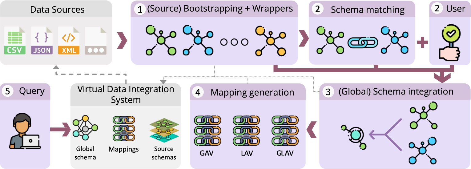
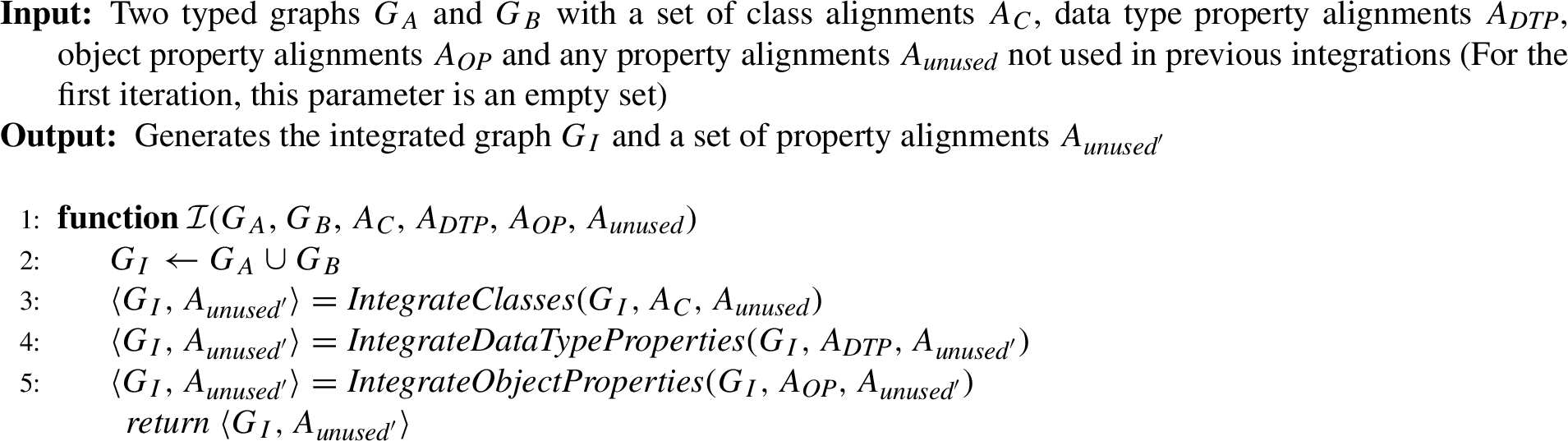
Data integration encompasses three main tasks: schema integration, record linkage, and data fusion [15,54]. In this paper, we focus on schema integration for virtual data integration to support flexible and on-demand data wrangling. We thus address the problem of automating the extraction of schemata from the sources, as well as their homogenization and integration [7]. The required constructs needed to enable schema integration have been properly studied in the literature [37]: the data source schemata, the target or integrated schema, mappings between the source and target schemata and wrappers fetching the actual data residing in the data sources. Figure 1 exemplifies the traditional steps conducted to build them. The process begins with a (1) bootstrapping and wrapper generation phase, which extracts a schema representation of each source and the program that allows fetching its data. Next, a (2) schema matching phase finds overlapping concepts among different sources, in order to later integrate them. (3) Schema integration is an iterative, user-supervised and incremental task, completed when all source schemata have been integrated into a single and unified global schema. The final phase consists of the (4) generation of mappings, which relate the global schema back to the sources. Virtual data integration systems rely on these constructs to, via rewriting algorithms, automatically rewrite queries over the global schema into queries over the sources [37]. The processes described above do neither support record linkage nor data fusion, which fall out of our scope. Oppositely to a traditional scenario, where all data sources were static, homogeneous and under control of the organization, having a dynamically evolving and heterogeneous set of data sources yields new challenges to efficiently implement such pipeline. We identify the following three:
1. The variety of structured and semi-structured data formats hamper the bootstrapping of the source schemata into a common representation (or canonical data model) that facilitate their homogenization.
2. Instead of the classical waterfall execution, the dynamic nature of data sources introduces the need for a pay-as-you-go approach [25] that should support incremental schema integration.
3. The large number and variety of domains in the data sources, some of them unknown at exploration time, hinders the use of predefined domain ontologies to lead the process.
Fig. 2.
Our approach in a nutshell.
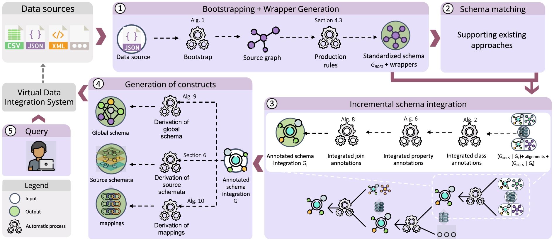
The limitations highlighted above have seriously hampered the development of end-to-end approaches for schema integration, which is a major need in practice, especially when facing Big Data [22,46]. To that end, we propose an all-encompassing approach that largely automates (essential for Big Data scenarios) schema integration. On top of that, we also implement our approach as an open-source tool called
Contributions We summarize our contributions as follows:
– Our approach is able to deal with heterogeneous and semi-structured data sources.
– It follows an incremental pay-as-you-go approach to support end-to-end schema integration.
– It provides a single, uniform and system-agnostic framework grounded on knowledge graphs.
– We developed and implemented novel algorithms to largely automate all the required phases for schema integration: 1◯ bootstrapping (and wrapper generation) and 3◯ schema integration.
– Our approach is not specific for a given system and it generates system-agnostic metadata that can be later used to generate the 4◯ specific constructs of most relevant virtual data integration systems. We showcase it by generating the specific constructs of two representative families of virtual data integration systems (an ontology-based data access system and a mediator-based system).
– We introduce
Reproducibility and code repository In an attempt to maximize transparency and openness,
Outline The rest of the paper is structured as follows. We first discuss the related work in Section 2. Next, Section 3 presents the formal overview of our approach to further dive in its two main stages: data source bootstrapping (Section 4) and schema integration (Section 5). Section 6 shows how our approach is able to the constructs required by data integration engines. Our approach implemented by
2.Related work
Data integration encompasses three main tasks: schema integration, record linkage, and data fusion [15,54]. A wealth of literature has been produced for each of them. In this paper, we focus on automating and standardizing the process to create the schema integration constructs for virtual data integration systems. Accordingly, in this section, we discuss related work on the two main phases depicted in Fig. 2: bootstrapping and schema integration. We wrap up this section discussing the available virtual data integration systems that provide some kind of support to generate the necessary schema integration constructs.
2.1.Related work on bootstrapping
Bootstrapping techniques are responsible for extracting a representation of the source schemata and there has been a significant amount of work in this area, as presented in several surveys [2,23,27,52]. Most of the current available efforts, however, do require an a priori available target schema and/or materialize the source data in the global schema [8,14,36]. Since our approach is bottom-up and meant for virtual systems, we subsequently focus on approaches generating the schema from each source (either checking the available metadata or instances) without using a reference schema or ontology. Table 1 depicts the most representative ones. To better categorize them, we distinguish three dimensions: required metadata, supported data sources, and implementation, which we detail as follows, accompanied by a discussion to highlight our contributions.
Table 1
Comparison of bootstrapping state-of-the-art techniques
| Approach | Required metadata | Supported data model | Implementation | |
| Availability | Automation | |||
| IncMap [48] | RDB Schema | Relational | Unknown | Semi-automatic |
| BootOX [31] | RDB Schema | Relational | Unavailable | Automatic |
| Janus [6] and XS2OWL [57] | XML Schema | XML | Unknown | Automatic |
| DTD2OWL [56] | DTD Schema | XML | Unknown | Automatic |
Required metadata All approaches define transformation rules to generate the schemata from the available data source metadata as in [6,8,57], and [56]. However, these transformation rules do require well-defined schemata, even for semi-structured data sources such as XML, which is not realistic for data wrangling tasks. Another relevant problem we identified in all these approaches is the lack of standardization of both the process and the generated schemata. All of them present ad-hoc rules that are not compliant with both the data source metamodel and, importantly, the target metamodel (typically, RDFS or OWL). This hinders the reuse and interoperability of these approaches within the end-to-end schema integration process. Indeed, the same schema processed by different approaches may result in different outputs. This is aligned with the current efforts on schema integration, which are specific for a project and do not generalize well.
Supported data sources Most approaches focus on bootstrapping relational data sources, assuming a traditional data integration setting, and only three support semi-structured data models [6,56,57] (in all cases, XML). Yet, in data science, most of the data available comes in the form of semi-structured data sources (e.g., JSON and CSV).
Implementation Current approaches do not provide an open implementation. BootOX [31] is integrated into Optique system [19], but it is no longer maintained or publicly available.
Discussion Our bootstrapping proposal differs from the state-of-the-art as follows: (1) the schema is extracted from the physical structure of the available data (i.e., instances) without relying on a pre-defined available schema of the source, (2) the process and produced schema are standardized. Specifically, our transformation rules are defined at the metamodel level and guarantee the output generated is compliant with both the data source and target metamodels. Standardization is key for efficient maintenance and its reuse in the subsequent schema integration phase, and (3) our approach is generic and adaptable to any data source data model. For those models not considered, we could extend our approach by providing a set of transformation rules satisfying the soundness and completeness properties defined in Section 4. Note that these rules are per pair of metamodels and therefore reusable between sources of the same format.
2.2.Related work on schema integration
Schema integration is the process of generating a unified schema that represents a set of source schemata. This process requires as input semantic correspondences between their elements (i.e., alignments). In Table 2, we depict the most relevant state-of-the-art approaches. We distinguish three dimensions: integration type, strategy, and implementation:
Table 2
Comparison of schema integration state-of-the-art techniques
| Approach | Integration type | Strategy | Implementation | |||
| Alignments preservation | Source schema preservation | Incremental | Availability | Automation | ||
| PROMPT [44] | Full merge | Archieved | Semi-automatic | |||
| Chimaera [39] and FCA-Merge [55] | Full merge | Unknown | Semi-automatic | |||
| ONION [40] | Simple merge | ✓ | ✓ | Unknown | Semi-automatic | |
| OntoMerge [16] | Simple merge | ✓ | ✓ | Unavailable | Automatic | |
| ATOM [51] | Asymmetric merge | ✓ | Unknown | Semi-automatic | ||
| CoMerger [5] | Full merge | ✓ | ✓ | Active | Automatic | |
| Chevalier et. al [58] | Full merge | ✓ | ✓ | Unknown | Semi-automatic | |
Integration type We follow the classification presented in [45], which categorizes the kinds of integration into three types, namely: simple merge, full merge, and asymmetric merge. The former integrates schemata by adding one-to-one bridge axioms between pairs of schemata. Approaches such as [40] and [16] preserve the original source schemata and alignments, which is a desirable property to manage source evolution [4] and mandatory for incremental approaches. However, their main drawback is the lack of common concepts, which can lead to complex queries when integrating a large number of schemata. Full merge integrates the source schemata generating a new schema where equivalent concepts are merged into a single new concept. In most approaches, the original source schemata is not preserved and therefore lost. Thus, these approaches are not incremental. [5] is the only approach under this category able to preserve specific elements of the source schemas upon request. Asymmetric merge can be performed using the simple and merge schema via one-to-many axioms to integrate schemas and derive a full merge. To the best of our knowledge, [51] is the only approach in this category. This kind of merge prioritizes one of the schemas (target) over the others (source), that is, the target schema will preserve all axioms and in case of disagreement with the target schema, elements of the source schema are removed from the integration.
Incremental integration Most approaches (e.g., [16,44,55]) integrate the source schemata in one shot. Thus, to process a new data source the whole process is started from scratch without reusing the previously generated structures. Instead, [51] reuses the integrated structure to facilitate further integration incrementally. To that end, it adopts the asymmetric merge strategy, however, it only supports the integration of taxonomies (i.e., classes with no attributes and only hierarchical relationships among them).
Implementation All approaches provide tools, however only [5] is openly available. There exists a demo of [16] on its website,66 however, as of today the service is down. Regarding [44], it is available as a plugin to the Protégé tool, however it is not longer maintained. Overall, we also encountered that none of the tools offer any documentation for users making them hard to use.
Discussion Our work differs from these works as follows: (1) the global schema is incrementally generated, rather than generated in one shot. (2) We thus incrementally support the integration of any resource (e.g., rdfs:Class and rdf:Property) rather than just focusing in one resource as in [51] (3) In contrast to any other approach, we generate annotations (i.e., metadata) and preserve the original schemata and alignments. These metadata are agnostic of the virtual data integration system at hand, and we are able to derive generic system-specific constructs from our system-agnostic annotations.
2.3.Related work on data integration systems supporting bootstrapping and/or schema integration
We examined virtual data integration systems that have introduced a pipeline supporting bootstrapping and/or schema integration with the goal of providing query access to a set of data sources. We have excluded systems that rely on the manual generation of schema integration constructs [11,41] and focus on those that support semi-automatic creation of such constructs.In all cases, nevertheless, the processes introduced are specific and dependent on the virtual data integration system at hand. Further, note that some popular data integration systems such as Karma [36], Pool Party Semantic [53], or Ontotext77 are excluded since they only support physical integration. Table 3 summarizes such efforts.
Table 3
Comparison of virtual data integration systems automating, at least partially, schema integration
| Approach | End-to-end DI workflow | Bootstrapping step | Schema integration | Implementation | ||||||
| Bootstrapping | Schema matching | Schema integration | Query | Type | Supported data sources | Type | Incremental | Availability | Last maintenance | |
| Optique [19] | ✓ | ✓ | ✓ | Provided and extracted | Relational, sensor data and streaming | Simple merge | – | On request (demo) | 2016 | |
| Mastro Studio [12] | ✓ | ✓ | Provided | Relational | – | Commercial use | Unknown | |||
Optique [19] It is a virtual data integration system developed as a result of research and industrial projects (e.g., [35]). For each data source, the source schema and RML mappings are generated using BootOX. In order to integrate schemata, equivalent resources between the source and global schemas are mapped manually. During this process, there is no matching technique. Moreover, the global schema is fully maintained by the user, who must update it if it is incomplete with respect to the data sources and propagate the changes throughout the system constructs. However, creating the system constructs does not follow an incremental process. Therefore, new constructs, which are tightly coupled with the system, are needed each time a new data source is added, or the global schema is updated. Finally, Optique allows the integration of relational, streaming, and sensor data and provides a query interface which is performed by the Ontop tool [11].
Mastro studio [12] It is a virtual data integration system currently available as commercial software maintained by OBDA Systems. The system supports only relational databases, which are mapped to a provided global schema. The mappings are defined in the system’s native language, making them tightly coupled to the system. Moreover, there are no schema matching and schema integration phases as it is assumed the user will provide the global schema. Thus, the main complexity is maintaining the global schema and mappings. The query phase explodes the ad-hoc mappings to provide a more efficient query retrieval.
Discussion All systems generate constructs tightly coupled with the system needs and assume a provided global schema. We, instead, construct the global schema incrementally from the sources, which is crucial for data wrangling. In these approaches, there are three common problems: (1) maintaining the mappings when the schema evolves, (2) updating the global schema to get a complete view of the data sources, and (3) incrementally generating all systems constructs. These problems are even more complex for all the other approaches (e.g., systems and query engines) that fully rely on creating such constructs manually [10,11,17,38,42,50]. Our approach is the only one incrementally generating and propagating changes. Further, we are not tied to any system. Our approach generates and collects rich metadata from the bootstrapping and schema integration steps. These metadata are rich enough to generate system-specific constructs for schema integration, as we show in Section 6. Our generic metadata is able to capture the evolution and automates its maintenance. Thus, if we need to update the constructs generated for a specific system, we only need to re-run the algorithms to produce the specific constructs and replace them in the system. Moreover, as integration is performed bottom-up, generating a global schema will always be complete with respect to the data sources, which is the main requirement for data wrangling.
3.Approach overview
We now introduce the formal overview of our approach and the running example used in the following sections.
3.1.Formal definitions and approach overview
3.1.1.Data source bootstrapping and production rules
Here, we present the formal definitions that are concerned with phase 1◯ as depicted in Fig. 2.
Datasets Let
Typed graphs We consider RDF graphs
Bootstrapping algorithm A bootstrapping algorithm for a data model m is a function
Graph queries We consider the query language of conjunctive graph queries (CQs) as defined in [9]. Formally, a CQ Q is an expression of the form
Production rules Let
3.1.2.Integrating bootstrapped graphs and generating the schema integration constructs
Here, we present the formal definitions that are concerned with phases 2◯, 3◯ and 4◯ as depicted in Fig. 2.
Alignments An alignment between two graphs
Graph integration algorithm A graph integration algorithm is a function
Schema integration constructs and their generation We follow Lenzerini’s general framework for schema integration88 [37]. Hence, a schema integration system
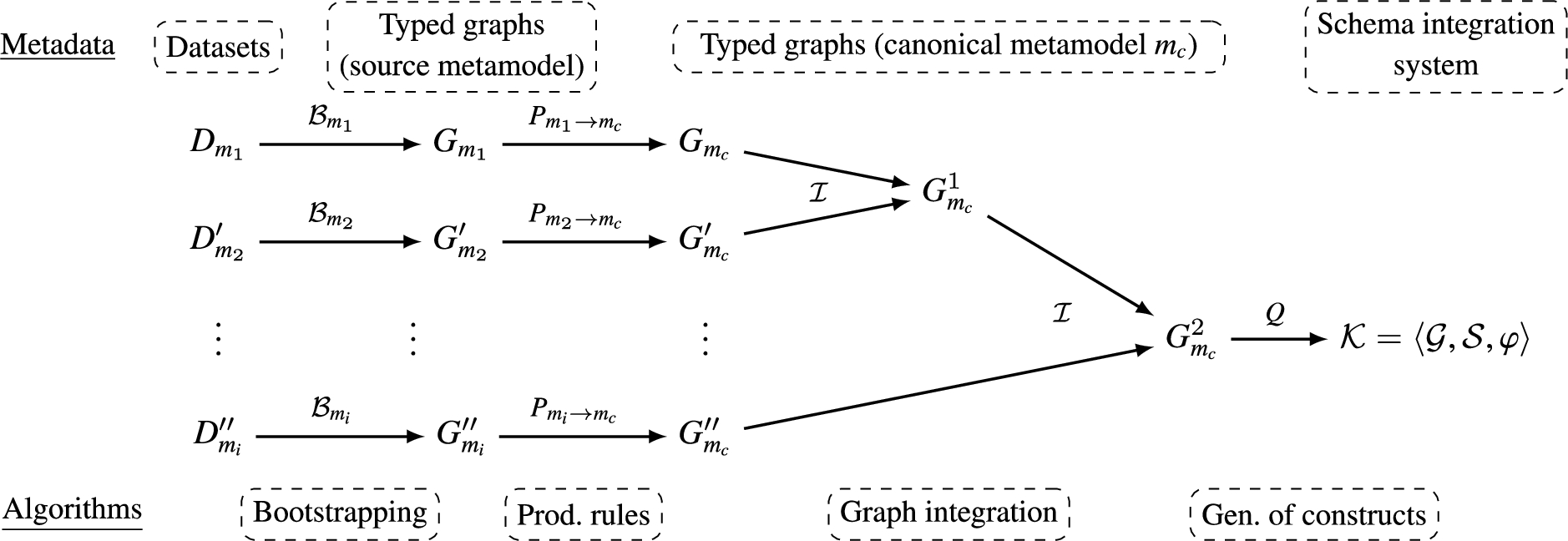
Overview of our approach Figure 3, summarizes the formal background introduced above and overviews our approach to automate the generation of schema integration constructs from a set of heterogeneous datasets.Shortly, for each dataset
Fig. 3.
Formal overview of our approach.
3.2.Running example
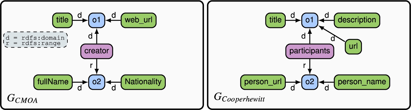
We consider a data analyst interested in wrangling two different sources about artworks from the Carnegie Museum of Art (CMOA)99 and Cooper Hewitt Museum (Cooperhewitt).1010 The former contains information such as the title, creator, and location for all artworks in the museum, such as fine arts, decorative arts, photography, and contemporary art. The latter contains similar information about artworks exposed in the Cooper Hewitt museum such as painted architecture, decorative arts, sculpture and pottery. Figure 4, depicts a fragment of the data in JSON format. Throughout the following sections, we will use this running example to showcase how our approach yields, from these semi-structured data sources, a schema integration system grounded on the previously introduced definitions.
Fig. 4.
Running example excerpts.
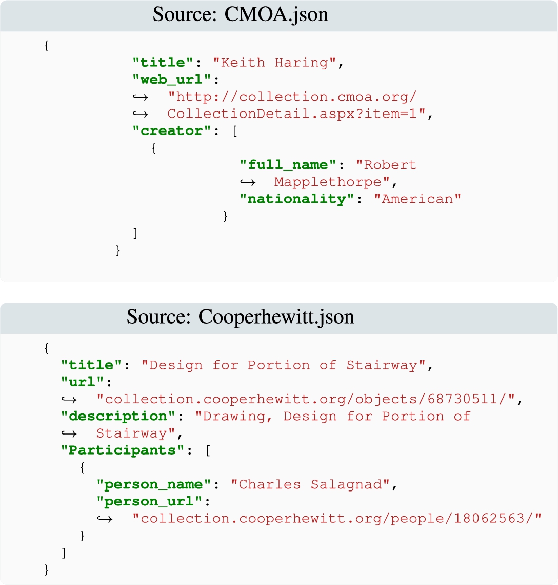
Fig. 5.
Metamodel to represent graph-based schemata of JSON datasets (i.e.,
![Metamodel to represent graph-based schemata of JSON datasets (i.e., MJSON) inspired from [29].](https://ip.ios.semcs.net:443/media/sw/2024/15-3/sw-15-3-sw233347/sw-15-sw233347-g005.jpg)
4.Data source bootstrapping
As previously described, our approach is generic to any data source, as long as specific algorithms are implemented and shown to satisfy soundness and completeness. In this section, we describe phase 1◯ in Fig. 2 and showcase a specific instantiation of the framework for JSON. Following Fig. 3, we introduce a bootstrapping algorithm that takes as input a JSON dataset and produces a typed graph-based representation of its schema. Then, such graph is translated into a graph typed with respect to a canonical data model by applying a sound set of production rules. Next, we present the metamodels required for our bootstrapping approach and the production rules.
4.1.Data source metamodeling
In order to guarantee a standardized process, the first step requires the definition of a metamodel for each data model considered (note that several sources might share the same data model). Figure 5 depicts the metamodel to represent graph-based JSON schemata (i.e.,  consists of one root
  , which in turn contains at least one
  instance. Each
  is associated with one
  value which is either a
  , a
, a  or a
or a  . We also assume elements of a
  to be homogeneous, and thus it is composed of
  elements. Last, we consider three kinds of primitives: these are
  ,
,  and
and  . In Appendix A, we present the complete set of constraints that guarantee that any typed graph with respect to
4.2.The canonical metamodel
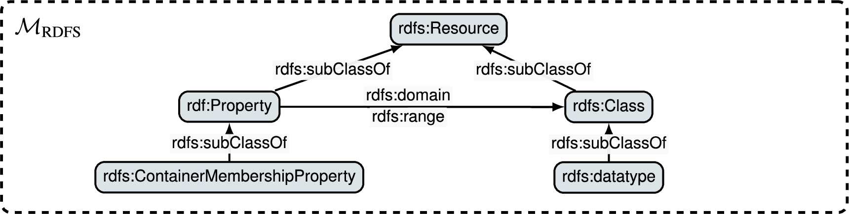
In order to enable interoperability among graphs typed w.r.t. source-specific metamodels, we choose RDFS as the canonical data model for the integration process. A significant advantage of RDFS is its built-in capabilities for meta-modeling, which supports different abstraction levels. Figure 6, depicts the fragment of the RDFS metamodel ( and their
  . Additionally, in order to model arrays and under the assumption that there exists a single type of container, we make use of the
  property. In Appendix B, we present the complete set of constraints that guarantee that any typed graph with respect to
Fig. 6.
Fragment of the RDFS metamodel (i.e.,
4.3.Bootstrapping JSON data
We next present a bootstrapping algorithm to generate graph-based representations of JSON datasets. The generation of wrappers that retrieve data using such graph representation has already been studied (e.g., see [42]), and here we reuse such efforts. Here, we focus on the construction of the required data structure. As depicted in Algorithm 1, the method
The goal of this algorithm is to instantiate the  and
and  elements using the document’s root. Then, the method Object recursively instantiates
  , we define its corresponding
 or
or  with fresh IRIs (i.e., object or array identifiers). This is not the case for primitive elements, which are either connected to the three possible instances of
  (i.e.,
  ,
,  , or
, or  ). The presence of such three possible instances in G is guaranteed by function
  to an instance of
  using the
  labeled edge.
Algorithm 1
Bootstrap a JSON dataset
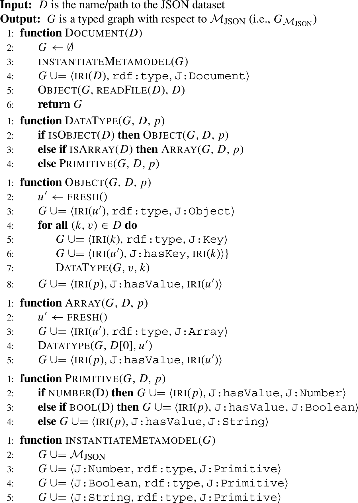
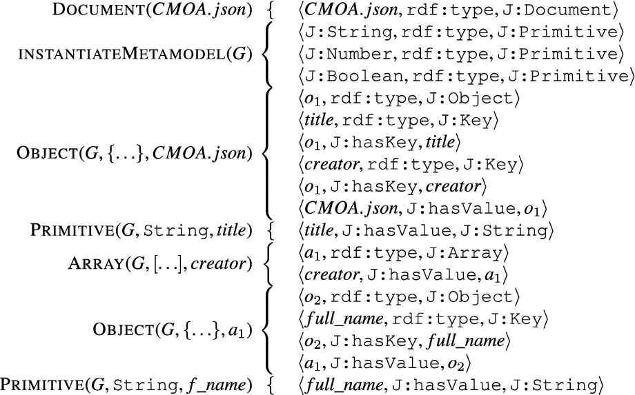
Example 1.
Retaking the running example introduced in Section 3.2, Fig. 7 depicts the set of triples that are generated by Algorithm 1 on a simplified version of the CMOA.json dataset. Note that, for the sake of simplicity, the keys web_url and nationality have been omitted.
Proof of soundness We show that Algorithm 1 is  are declared in line 4 of function Document, while all instances of
  and
and  are declared, respectively, in lines 3 and 5 of function Object. Instances of
  are declared in line 3 of function Array. Regarding primitive data types, they are all declared once when instantiating the metamodel.
Fig. 7.
Set of triples generated by Algorithm 1. In the left-hand side we depict the function that generates each corresponding set of triples.
Proof of completeness We show that Algorithm 1 is complete with respect to the JSON dataset. That is, for any JSON key k, there exists a resource R in the generated graph. This is guaranteed since for every element in  ,
,  ,
,  ,
,  and
and  there exists a method named likewise. Regarding
  , the resource R is created in the method Object. Note that we assume keys in a JSON dataset contain schema values and not data values (i.e., they are well-formed). We also assume that all elements in an array are homogeneous.
4.4.Production rules
We next present the second step of our bootstrapping approach (see Fig. 3), which is the translation of graphs typed with respect to a specific source data model (e.g.,
Rule 1.
Instances of  are translated to instances of
  .
.
Rule 2.
Instances of  are translated to instances of
  . Additionally, this requires defining the
  of such newly defined instance of
  .
.
Rule 3.
Instances of  which have a value an instance of
  are also instance of
  .
.
Rule 4.
The  of an instance of
  is its corresponding counterpart in the xsd vocabulary. Below we show the case for instances of
  whose counterpart is
  . The procedure for instances of
  and
and  is similar using their pertaining type.
Rule 5.
The  of an instance of
  is the value itself.
Example 2.
Here, we take as input the graph generated by our bootstrapping algorithm depicted in Fig. 7. Then, Fig. 8 shows the resulting graph typed w.r.t. the RDFs metamodel after applying the production rules. Each node and edge is annotated with the rule index that produced it.
Fig. 8.
Graph typed w.r.t. the RDFS metamodel resulting from evaluating the production rules.
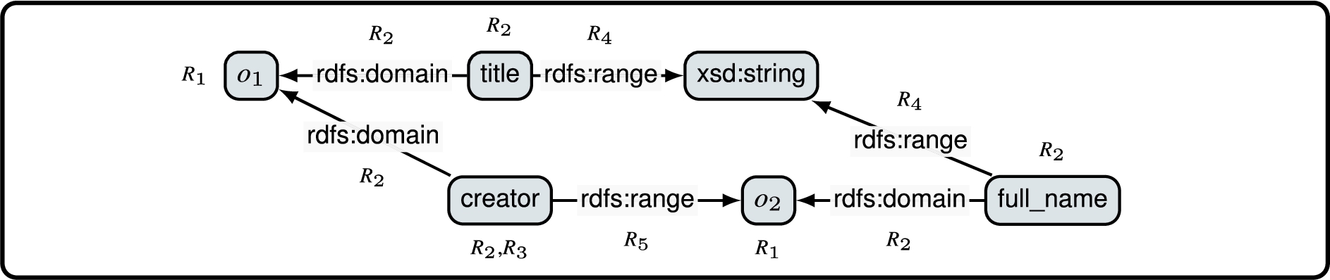
Fig. 9.
Extension of the rdfs metamodel for the integration annotation.

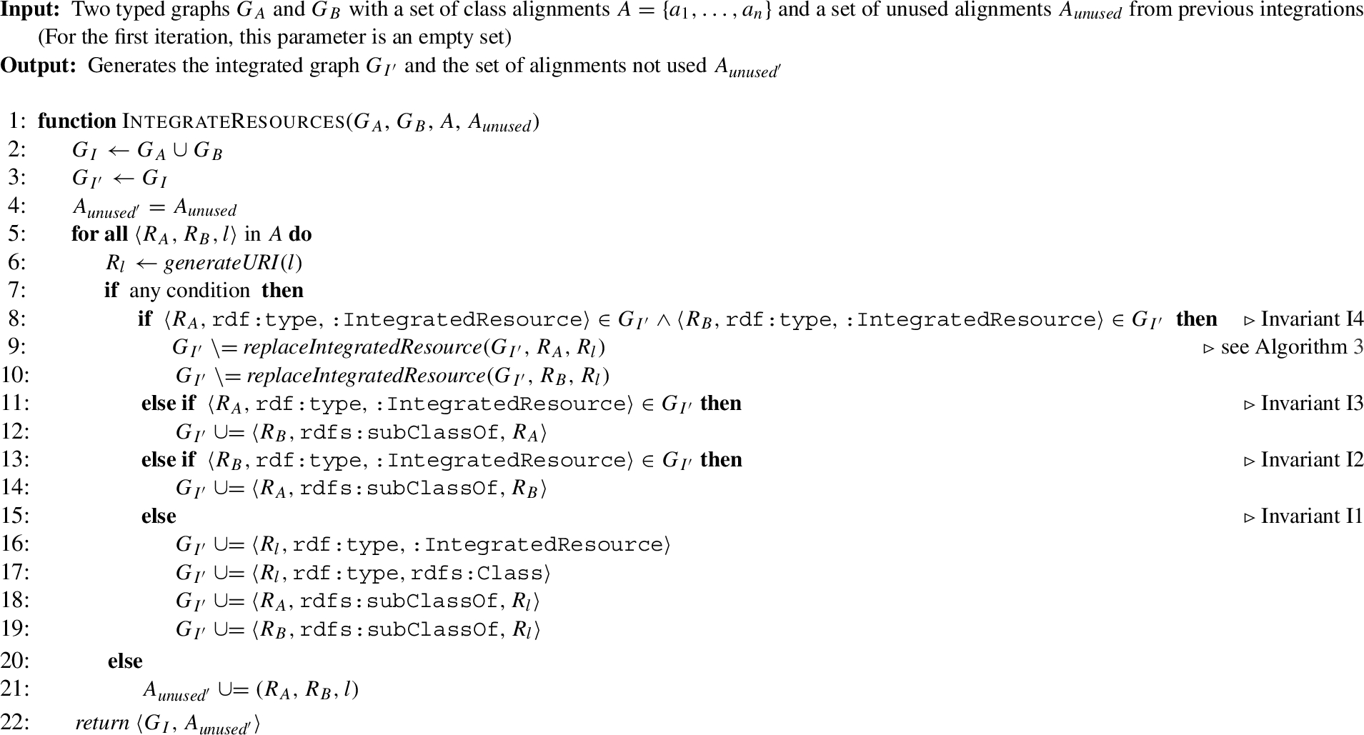
5.Incremental schema integration
This section describes phase 3◯ in Fig. 2, which addresses the problem of generating the integrated graph (IG) from a pair of typed graphs, as illustrated in Fig. 3. To facilitate the schema integration process, we extend the fragment of the RDFS metamodel (See Section 4.2) to include two new resources, namely  and
and  (see Fig. 9). These resources are essential to annotate how the underlying data sources must be integrated (e.g., union or join). The integration is accomplished through a set of invariants (see Section 5.1) that guarantee the completeness and incrementality of the IG. Importantly, our proposal is sound and complete with regard to the bootstrapping method described in Section 4 and it can only guarantee these properties if its input is typed graphs (see Fig. 3). The algorithm we propose in this phase takes as input two typed graphs and a list of semantic correspondences (i.e., alignments) between them. The integration algorithm is guided by semantic correspondences when generating the IG, keeping track of used and unused alignments in the process. Unused alignments identify those semantic correspondences not yet integrated due to conditions imposed by the integration algorithm, but to be integrated once the conditions are met in further executions. To obtain the semantic correspondences, we rely on existing schema matching techniques (e.g., LogMap [30] or
All in all, the IG is a rich set of metadata containing all relevant information to perform schema integration and, as such, it traces all information from the sources as well as that of integrated resources to support their incremental construction. In Appendix B.1, we present the complete set of constraints that guarantee that any IG is consistent.
Example 3.
Continuing the running example, Fig. 10 illustrates the result of the bootstrapping step to generate the typed graph representation of the data sources CMOA.json and Cooperhewitt.json. Note that the range properties are omitted due to space reasons. Also, we distinguish  and
and  . Since this information is not available in the input typed graphs, we use
  and distinguish them by checking their range. Hereinafter, as shown in Fig. 10, we use the following color schemes to represent
  ,
,  and
and  . We use dark colors to represent integrated resources:
  of type class,
  of type datatype property and
  of type object property.
Fig. 10.
The extracted canonical RDF representations for the CMOA and cooperhewitt sources.
5.1.Integration of resources
We here present an implementation for the graph integration algorithm (see Section 3.1.2). This algorithm, system-agnostic (i.e., not tied to any specific system) and incremental by definition, generates an integrated graph
I1 If  , then
I2 If  and
and  , then
I3 If  and
and  , then
I4 If  , then the new integrated resource
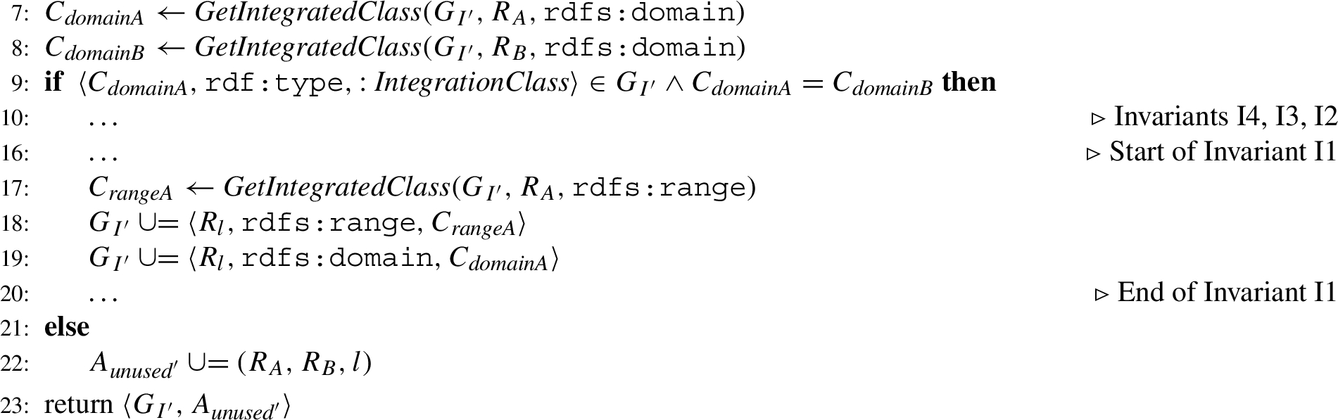
Intuitively, the presented invariants guarantee the soundness and completeness of our approach, since it covers all potential cases derived from one-to-one mappings: non-previously integrated resources, either one or another previously integrated or both already integrated. Grounded on these invariants, Algorithm 2 generates the corresponding integrated metadata and supports their incremental construction and propagation. Note that invariant I1 creates a new  of type class, invariants I2 and I3 reuse an existing
  and invariant I4 replace an
  . To accomplish I4, our algorithm uses the method replaceIntegratedResource depicted in Algorithm 3, which provides the necessary functionality to replace the resources that were integrated by an
  with
with  . When integrating classes, all resources (e.g., properties) connected to
  must be connected to
  For example, replacing an
  of type class requires updating all properties referencing
  by rdfs:range or rdfs:domain to reference
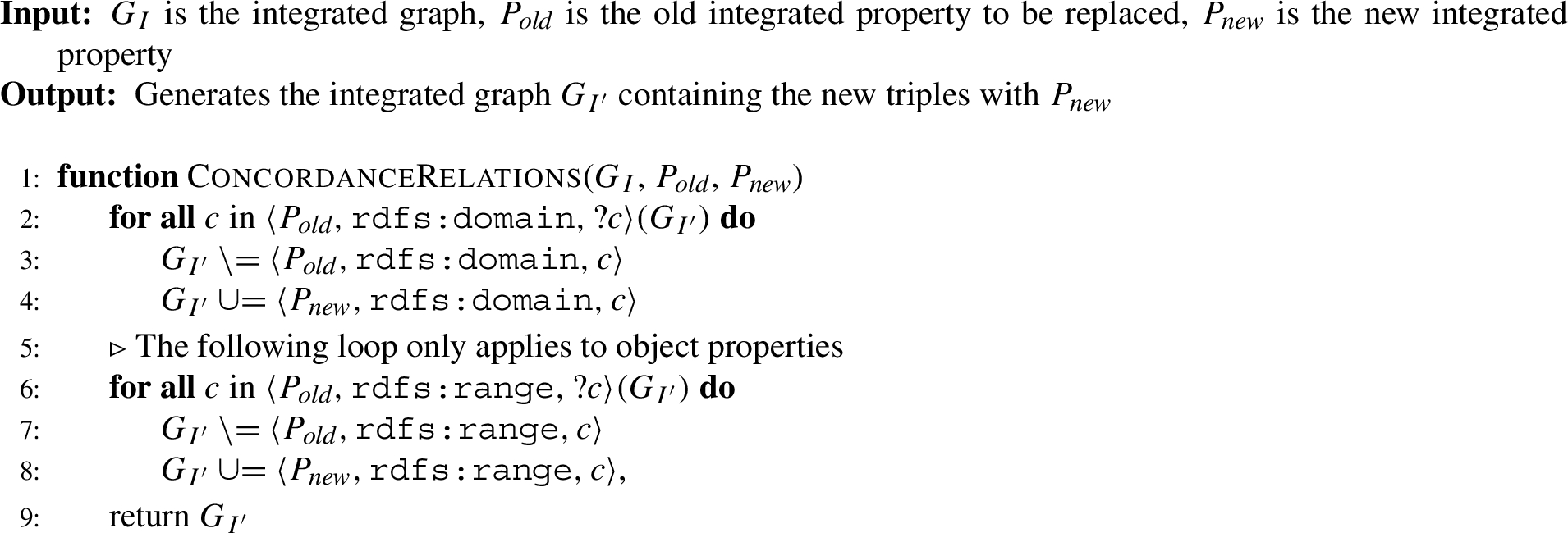
  . Therefore, we introduce the method concordanceRelations to redirect the relations from an old resource to a new resource.
Algorithm 2
Integration of resources – classes
Algorithm 3
Replace integrated resource – classes
Algorithm 4 is the main integration algorithm to generate
5.1.1.Integration of classes
We have introduced the  axioms are coherent when replacing an
  .
.
Algorithm 4
Incremental schema integration.
Algorithm 5
ConcordanceRelations – classes.
Table 4
Discovered correspondences for
| User-provided label l | ||
 |  | Artworks |
 |  | Title |
 |  | URL |
 |  | Creator |
 |  | Name |
 |  | Contributors |
Fig. 11.
Integration of two classes from
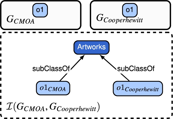
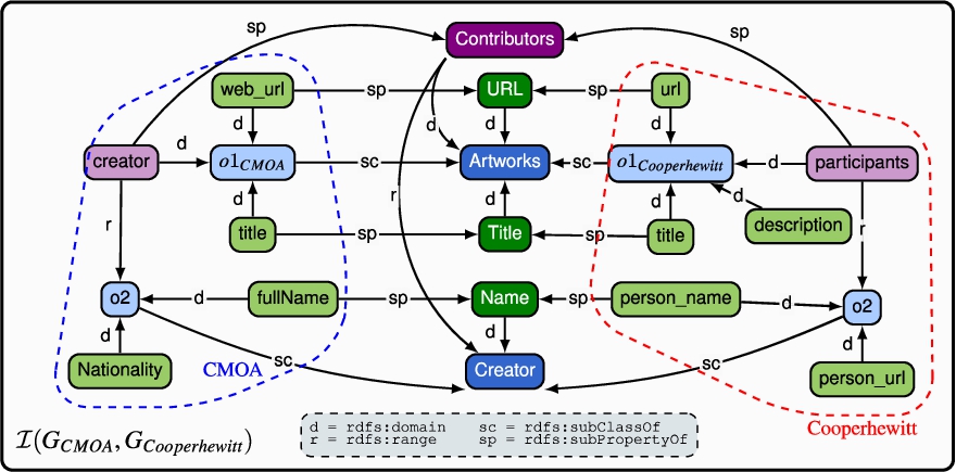
Example 4.
Retaking the running example, consider the alignments depicted in Table 4 between  and
and  . For this case, invariant I1 is applied as illustrated in Fig. 11. Thus, both classes are connected to a newly defined instance of class
  and
and  , namely
  . For this example, two
  were generated:
  and
and  . Note, the set
5.1.2.Integration of properties
The invariants for properties are very similar to those presented for classes. Thus, we will use the  and
and  .
.
Let us start with datatype properties. Following the class-oriented integration idea introduced, we only integrate datatypes if they are part of the same entity, that is, if their domains (e.g.,  ) have already been integrated into the same
  of type class. Therefore, the invariants for
  integration must reflect this condition. In the following, we present invariant I1 for
  . Note that the remaining invariants should be updated accordingly.
Algorithm 6 implements the IntegrateDataTypeProperties method in Algorithm 4. The implementation of IntegrateDataTypeProperties method is similar to Algorithm 2 except for the additional conditions and the manipulation of the domain and range axioms. If the conditions are not fulfilled, the algorithm does not integrate the alignment and preserves it in the set of  in further integrations. Thus, whether this integration will take place depends on the discovered set of alignments from the schema matching approaches. Further, the domain of the
  of type property is an
  of type class. And for the range, we assign the more flexible xsd type (e.g., xsd:string). Algorithm 7 implements the method concordanceRelations to ensure all axioms are coherent when replacing an
  or an
or an  of type property.
For the integration of  , we follow a similar approach and only integrate object properties if their domain and range have already been integrated. Accordingly, the object property invariants should reflect this condition and we showcase it for invariant I1 as follows:
Algorithm 7
ConcordanceRelations – properties.
The implementation of the  integration is very similar to Algorithm 6. We should accordingly add the proper conditions set by the invariants and consider the manipulation of the axioms as we performed for
  . We illustrate the integration of properties in Example 5.
Example 5.
Continuing the Example 4, the algorithm will integrate all  using invariant I1 since their domains were already integrated. If their domains are not integrated, the properties will be preserved in the set of unused alignments
  and
and  . The integration algorithm uses rdfs:subPropertyOf to connect both
  to the
  of type property, that is,
  . For this example, the following
  were generated:
  ,
,  and
and  . Then, we proceed to integrate
  as we can note that the domain and range of
  and
and 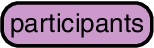 have already been integrated, fulfilling the object property requirement. Finally, Fig. 13 depicts the complete integrated graph generated from Example 4 and 5. The result of this schema integration generates one
  of type class, three
  of type datatype property and one
  of type object property. Note that the set
Fig. 12.
Result of integrating two classes and two data type properties from
Algorithm 8
Join integration
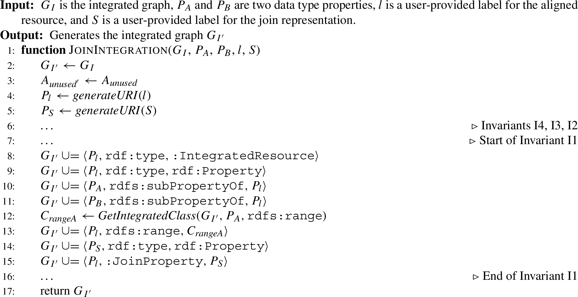
Fig. 14.
Example of a join integration.
Fig. 15.
New data source.
Table 5
Alignments discovered for
| User-provided label l | ||
 |  | Artist |
 |  | Nationality |
 |  | Name |
Fig. 16.
Result of integrating two integrated classes from
As discussed, our property integration is class-oriented and we only automate the process if the integrated properties are equivalent and can be integrated via a union operator. However, in real practice, this is very restrictive and we allow to integrate two datatype properties whose classes have not been previously integrated in what we call a  . This integration must be performed by a post-process task triggered by a user request. This type of property integration occurs when the domains are not semantically related, but the properties have a semantic correspondence in an input alignment. We thus consider this case as a join operation. Algorithm 8 depicts this integration type. Having no conditions allows us to integrate properties from completely distinct entities. To allow this integration, we must express the join relationship by creating an
  that connects both domain
  of the
  to integrate, as illustrated in Fig. 14. This object property aims to add semantic meaning to the implicit relation of the properties domain. Thus, this
  connects to the
  using
using  to identify that this is an on-demand datatype property integration not meeting the regular integration algorithms.
5.2.Incremental example
We will use the final result of Example 5 to perform an incremental integration. For this case, consider the data analyst wants to integrate the typed graph  . Let us consider the alignment
  and
and  . Note that we have two
  of type class in this alignment resulting in the use of invariant
  and
and  are replaced by the new
  of type class, namely
  . Now, the algorithm proceeds to integrate
  . Let us consider the alignment
  and
and  representing invariant
  of type property, we reuse
  . Therefore,
  will be a
 . For the last alignment,
  and
and  , we replace both
  of type property by
  . In summary, our approach creates one
  of type class and two
  of type property. The resulting integrated graph is depicted in Fig. 18.
Fig. 17.
Result of integrating one integrated data type property from
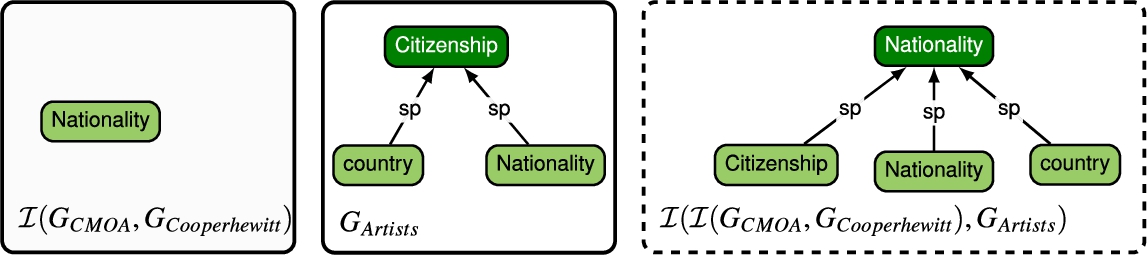
Fig. 18.
Integration graph from a second integration.
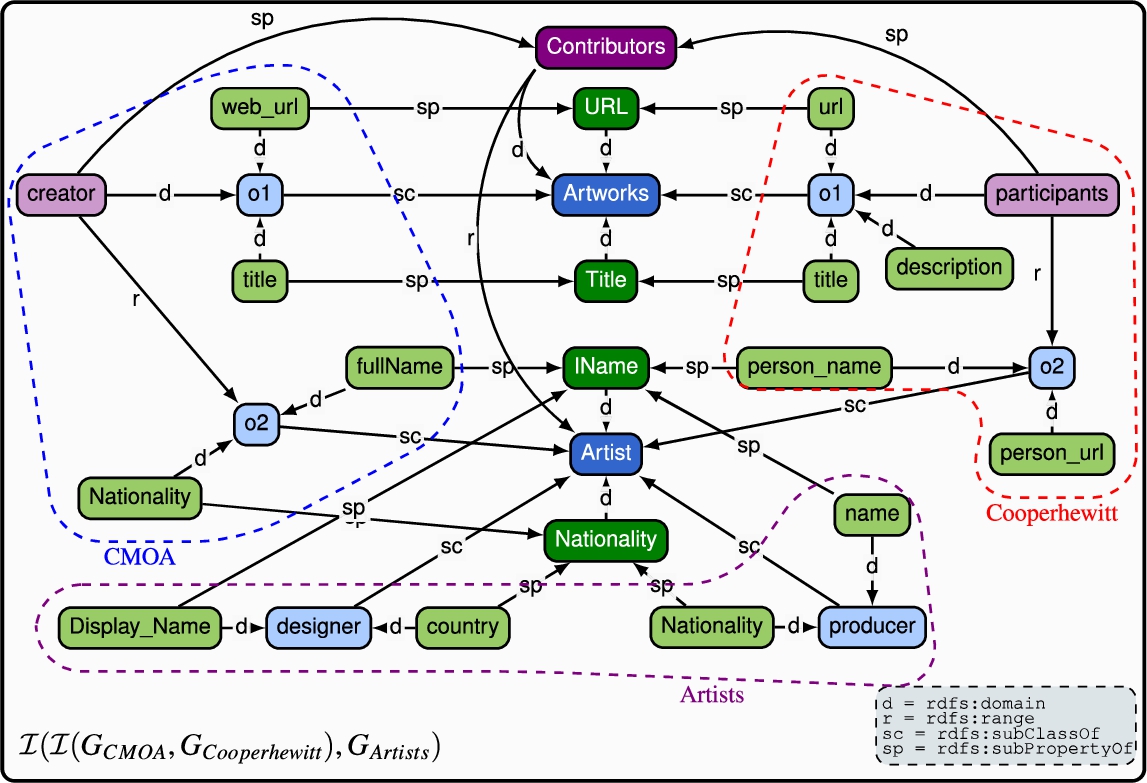
Fig. 19.
Example of two different data models.
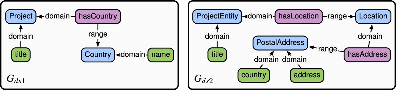
5.3.Limitations
The integration algorithm is our incremental proposal to integrate the typed graphs. However, this algorithm assumes one-to-one input alignments, a limitation all schema alignment techniques have. Our integration algorithm integrates equivalent resources, but it is not able to deal with other complex semantic relationships. To illustrate this, consider the example presented in Fig. 19. Let us consider a data analyst interested in retrieving the country’s name related to a project. For the  property to retrieve the
  entity. However, the
  entity, using the
  property, and then using the
  property to retrieve the
  entity, which contains the
  information. The main problem in this case is that the alignment is not one-to-one, instead, the alignment matches a subgraph to one resource. As far as we know, there is no schema alignment technique that considers such case and we for now do not either and leave it for future work. Last, but not least, we would like to stress that even if largely automated, schema integration must be a user-in-the-loop process, since this is the only way to guarantee the input alignments generated by a schema alignment tool are correct.
6.Generation of schema integration constructs
In this section, we show how our approach can be generalized and reused to derive the schema integration constructs of specific virtual data integration systems. We, precisely, instantiate phase 4◯ in Fig. 2. The integrated graph generated in Section 5 contains all relevant metadata about the sources and their integration, which can be used to derive these constructs. Regardless of the virtual data integration system chosen, once the system-specific constructs are created, the user can load them into the system and start wrangling the sources via queries over the global schema. This way, we free the end-user from manually creating such constructs. In the following subsections, we present two methods to generate the schema integration constructs of two representative virtual data integration approaches: mediator-based and ontology-based data access systems
6.1.Mediator-based systems
We consider ODIN as a representative mediator-based data integration system [43]. ODIN relies on knowledge graphs to represent all the necessary constructs for query answering (i.e., the global graph, source graphs and local-as-view mappings). However, all its constructs must be manually created. Thus, we show how to generate its constructs automatically from the integrated graph generated in our approach.
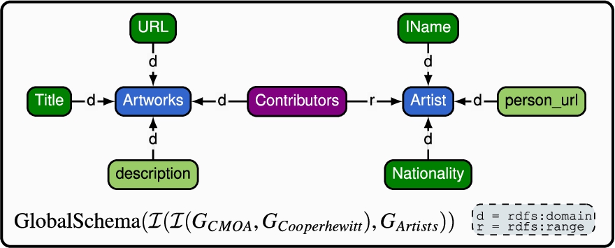
Algorithm 9 shows how to generate the global graph required by ODIN from our integrated graph. In ODIN, the global graph is the integrated view where end-users can pose queries. Hence, this algorithm first merges the sub-classes and sub-properties of integrated resources. As a result, we represent the taxonomy of integrated resources with a single integrated resource and properly modify the domain and range of the affected properties. In the case of non-integrated resources, their original definition remains. Figure 20, illustrates the output provided by Algorithm 9 for the generated integration graph in Fig. 18. The source schemata and wrappers representing the sources and required by ODIN are immediate to retrieve, since our integration schema preserves the original graph representation bootstrapped per source, and the wrappers remain the same. Finally, since the integration graph was built bottom-up, the local-as-view mappings required by ODIN are generated via the sub-class or sub-property relationships created during schema integration between source schemata elements and integrated elements. All ODIN constructs are therefore straightforwardly generated from the integration graph automatically. Once done, and after loading these constructs into ODIN, the user can query the data sources by querying the global graph of ODIN, which will rewrite the user query over the global graph into a set of queries over the wrappers via its built-in query rewriting algorithm. We have implemented the method here described to generate the constructs and integrated it in ODIN. This implementation is available on this paper’s companion website.
Algorithm 9
Global schema
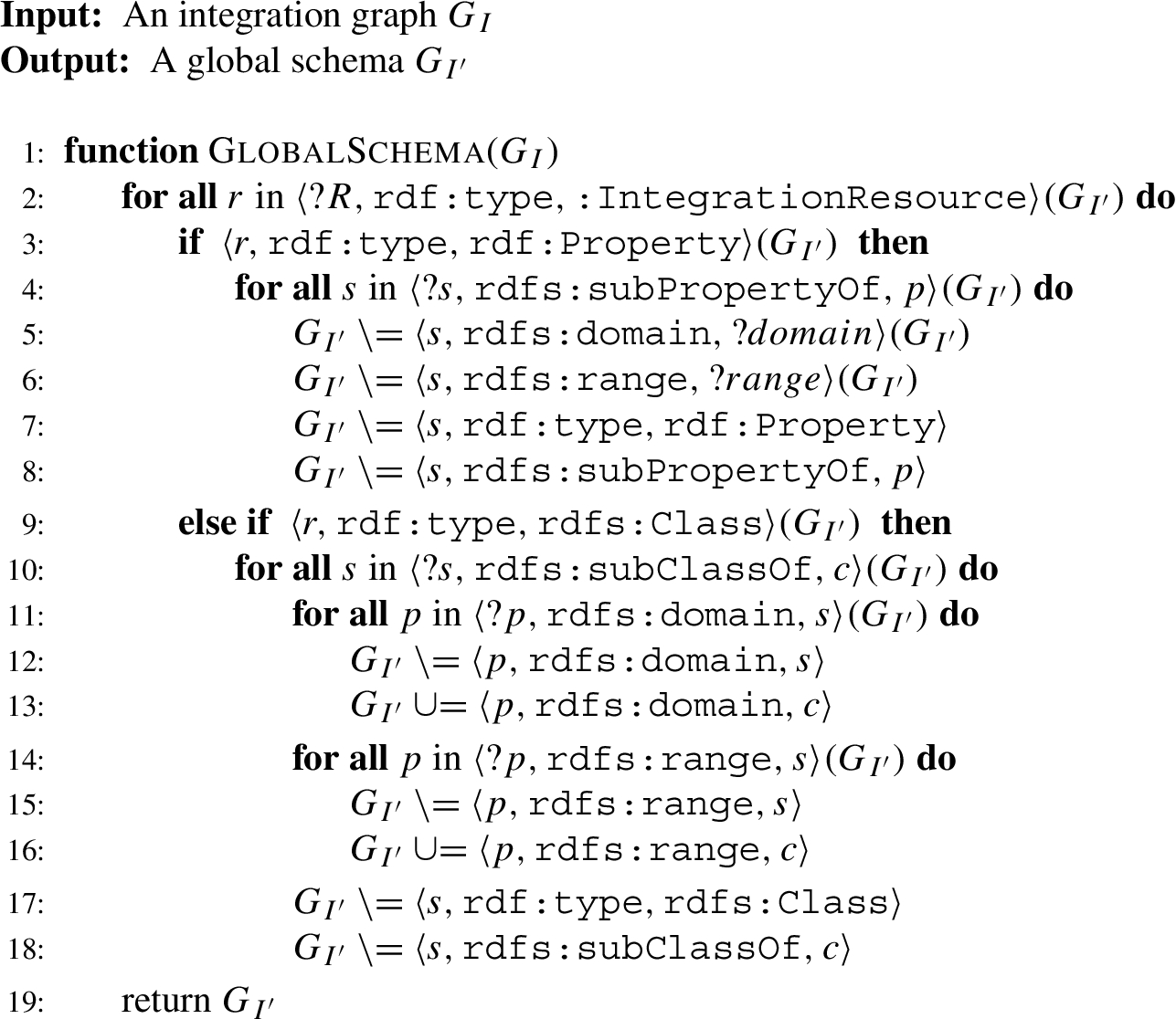
Fig. 20.
Generated global schema.
6.2.Ontology-based data access systems
Ontology-based data access systems provide a unified view over a set of heterogeneous datasets through an ontology, usually expressed in the OWL 2 QL profile, and global-as-view mappings, often specified using languages such as R2RML and RML. The integrated graph is able to derive an OWL ontology by converting RDFS resources into OWL resources. To this aim, Algorithm 9 requires a post-process step to perform this task. Note that, by definition, the integrated graph contains a small subset of RDFS resources. Thus, we only require to map  to
to  and
and  to the corresponding
  or
or  . Concerning mappings, as long as appropriate algorithms are defined to extract and translate the metadata from the integrated graph, we can derive mappings for any dedicated syntax. Here, we will explain the derivation of RML mappings. Each RML mapping consists of three main components: (i) the Logical Source (
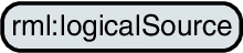 ) to specify the data source, (ii) the Subject Map (
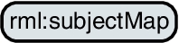 ) to define the class of the RDF instances generated and that will serve as subjects for all RDF triples generated, and (iii) a set of Predicate-Object maps (
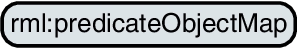 ) that define the creation of predicates and its object value for the RDF subjects generated by the Subject Map. Algorithm 10 shows how to generate RML mappings from the integrated graph. The process is as follows.
The algorithm creates RML mappings for each entity defined in a data source schema. Therefore, it iterates over all resources of type  from the integrated graph that are not
  , since those resources were generated from a data source during the bootstrapping phase. For each resource c of type
  , we generate a unique URI, namely
 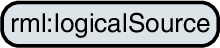 for the mapping
  to specify the data source location, which is obtained from the source wrapper through the method
  to express the data source format, which is assigned dynamically depending on the data source type by using the method
  or
or  ), and (iii) the
 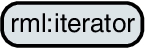 to define the iteration pattern to retrieve each data instance to be mapped, obtained from the wrapper definition using the method
Algorithm 10
RML mappings generation.
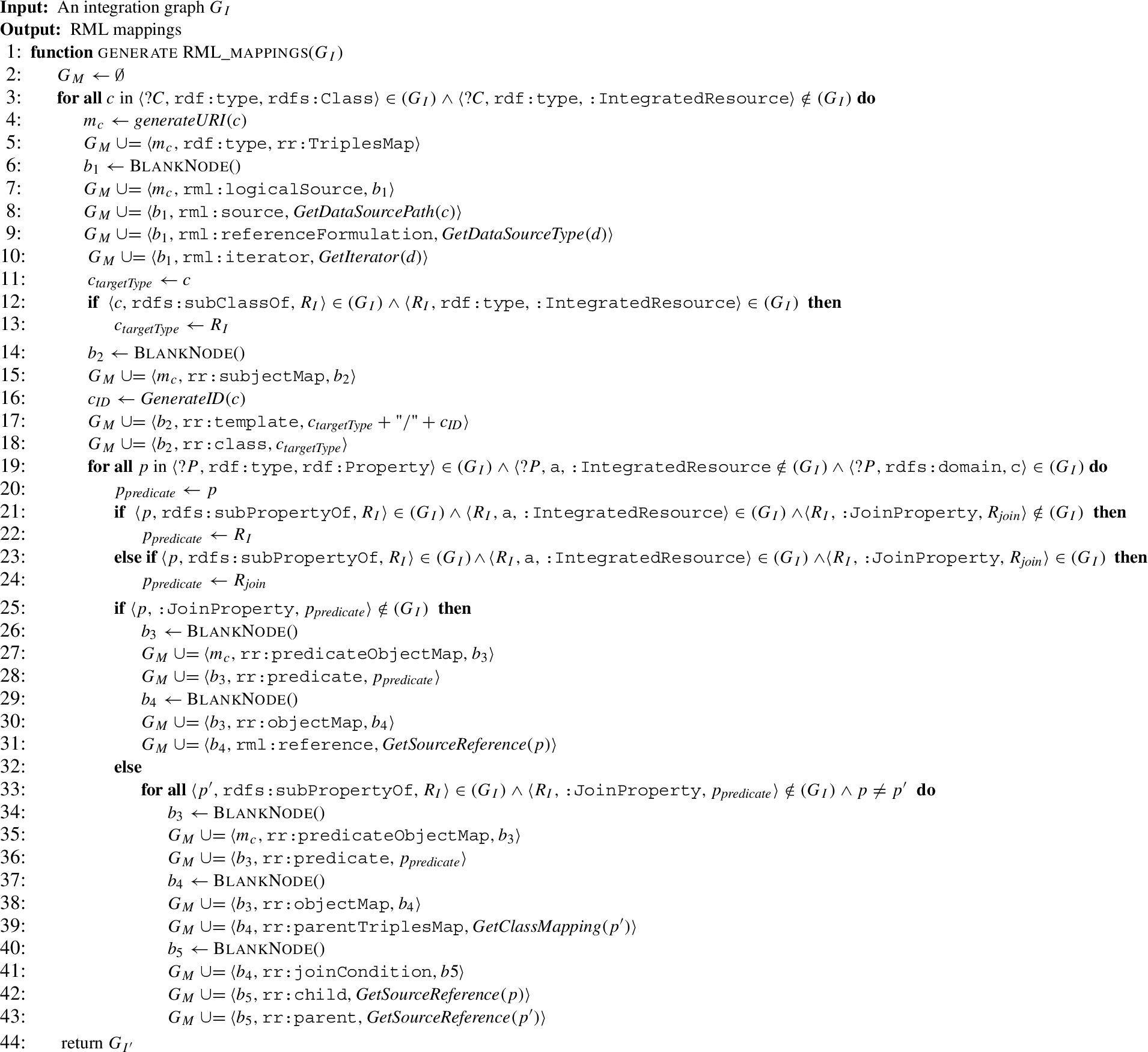
The next step is to specify the 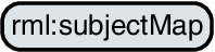 for the mapping
  , we define
  : (i) the
  to define the URIs of the instances, for which we use the URI from
  to specify the class of the subjects produced. Then, we create of the set of
  . To that end, we iterate over all
  that has as domain the class c. Then, for each property p, we define the variable
  or p is a subproperty of an
  that represents a
  , we define
  metadata. Here, we distinguish two cases: properties that are not part of a
  and those that are. In the first case, we will generate the metadata as follows: (i) the
  to indicate that property
  as well as
 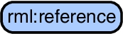 to indicate which element of the data source schema should be used to generate the RDF objects instances. Here, we use the method
  , we will create a
  for all properties that are part of the
  . Then, the following metadata is generated for each
 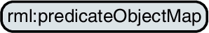 : (i) the
  where we use the join property URI to connect two entities from different sources, and (ii) the
  along with a
  , which is used to link the mappings of two different entities. We use the method
  : (i) the
  containing the
  and the
  , which require a reference of an element from the data source to create the join. We used the method
As a result, the provided algorithm generates the RML mappings for all entities and data sources contained in an integrated graph and uses the annotations with regard to unions and joins to construct global-as-view mappings according to the global schema (e.g., ontology). Last but not least, this algorithm showcases the feasibility of generating RML mappings from the integrated graph. Note that the generated RML mappings can be used for any RML compliant engines (virtual or materialized) such as Morph-RDB [49], RDFizer [28] and RMLStreamer [24]. Importantly, note that our objective is not to generate optimized RML mappings, which should be part of the future work.
7.Evaluation
In this section, we evaluate the implementation of our approach. To that end, we have developed a Java library named
– (Q1) Does the usage of
– (Q2) Does the usage of
– (Q3) Does the quality of the generated integrated schema improve using
– (Q4) Does the runtime of
To address questions Q1, Q2, and Q3, we conducted a user study. Note we distinguish between Q1 and Q2, since the first is meant to report on the qualitative perception (according to the feedback received), while Q2 is a quantitative metric independent of the participant feelings during the activity. Regarding Q4, we carried out scalability experiments.
7.1.User study
This user study aims at evaluating the efficiency and quality of
Data sources We selected four data sources collected from the Tate collection1313 and CMOA collection.1414 All data sources are modeled using JSON and contain distinct entities related to artworks and artists. The number of schema elements in each data source, are, respectively, 48, 30, 30, and 13.
Definition of the data collection methods As discussed in Section 2, no tool from the state-of-the-art covers the same end-to-end process as our approach does. Thus, as a baseline representation of the conventional schema integration pipeline, we designed a set of notebooks to support each of the tasks described above.1515 Such notebooks contain detailed instructions on how to use the RDFLib Python library for the generation of RDF data. We leveraged on our industrial partners to generate a realistic baseline. It is important to observe that CoMerger [5] could be used as part of the pipeline for schema integration, yet the lack of proper documentation and the large number of issues at execution time hindered its use. In order to evaluate
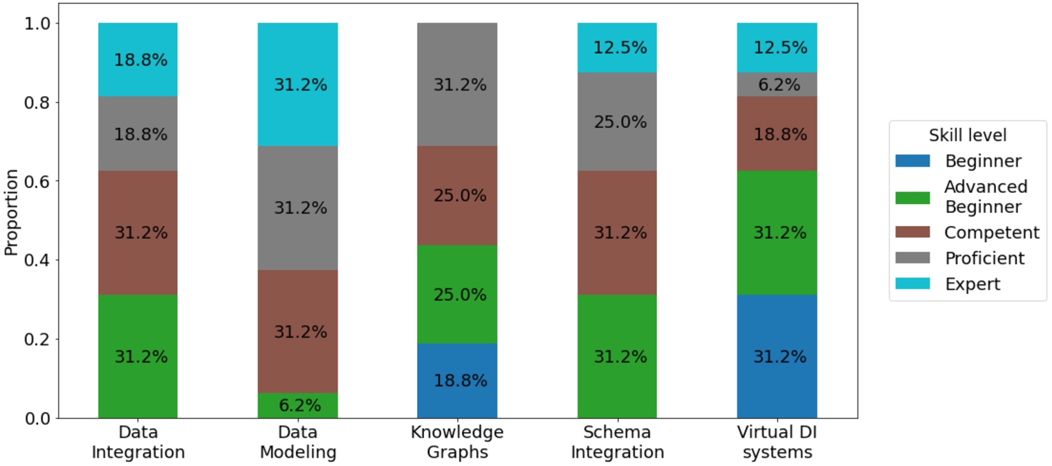
Selection of participants A set of 16 practitioners was selected to participate in the user study. Care was taken in selecting participants both from academia (researchers at UPC) and industry with different backgrounds and expertise (e.g., a broad range of skills, different seniority levels). All of them have participated in at least one Data Science project. Figure 21 summarizes how participants describe themselves with regard to the relevant skills required to perform the study. Specifically, we asked them to rate how skilled they felt in data integration (and specifically in the sub-domains of schema integration and virtual data integration systems), data modeling and knowledge graphs. All these skills were needed during the study and, as shown later, provide value when interpreting the results obtained. Participants were divided into two equally sized groups and assigned either v1 or v2.
Fig. 21.
Distribution of level across skills for all participants.
Evaluation of collected results In order to evaluate the results of each survey, we compare the aggregated answers for each non free-form question distinguishing between the conventional approach and
Fig. 22.
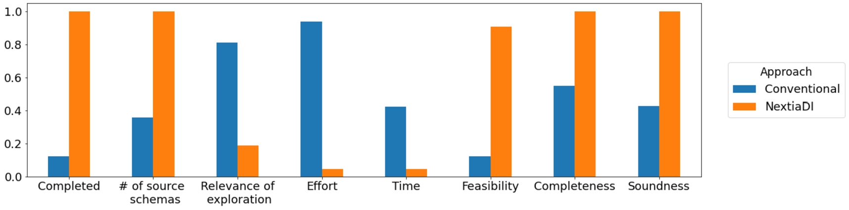
Aggregated results for the bootstrapping phase. Completed specifies whether participants finished the task within the available time (higher is better). # of source schemas denotes how many schema elements participants managed to bootstrap in the available time (higher is better). Relevance of exploration denotes the need a participant perceived to explore the structure of the sources to conduct the activity (lower is better). Effort and Time specifies, respectively, the perceived effort and time to complete the task (lower is better). Feasibility is used to quantify the perceived feasibility of running the task with the approach at hand (higher is better). Completeness and Soundness refer to the quality metrics previously introduced.
7.2.Analysis of results
Results on bootstrapping Figure 22 shows the aggregated results from the bootstrapping survey, where participants were required to define a graph-based schema for each data source with the two approaches. In the conventional approach, only 12.5% of the participants generated the four schemata, while using
Results on schema integration Figure 23 depicts the aggregated results for the schema integration survey, where participants were required to integrate the schemas generated in the previous task. In order to accomplish it, three main integrated schemata had to be created (i.e., DS1-DS2, DS1-DS2-DS3, and DS1-DS2-DS3-DS4). On the conventional approach, only 6.25% of the participants managed to generate the three integrated schemas. In contrast, using
Fig. 23.
Aggregated results for the schema integration phase. Completed specifies whether participants finished the task within the available time (higher is better). # of integrated schemas denotes how many schema elements participants managed to integrate in the available time (higher is better). Effort specifies perceived effort to complete the task (lower is better). Satisfaction is used to quantify the perceived satisfaction of running the task with each approach (higher is better). Completeness and Soundness refer to the quality metrics previously introduced.
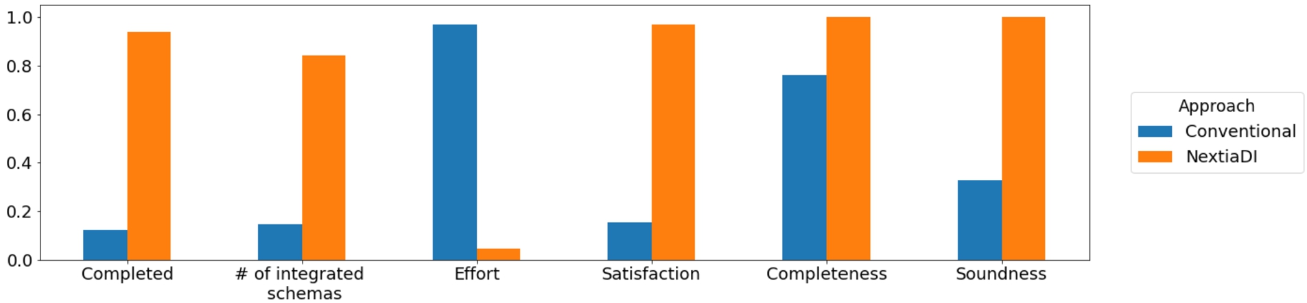
Fig. 24.
Aggregated results for the mapping generation phase. Completed specifies whether participants finished the task within the available time (higher is better). Effort and Time indicate, respectively, the perceived effort and time to complete the task (lower is better). Feasible is used to quantify the perceived feasibility of the task in Big Data settings (higher is better). Completeness and Soundness refer to the quality metrics previously introduced.
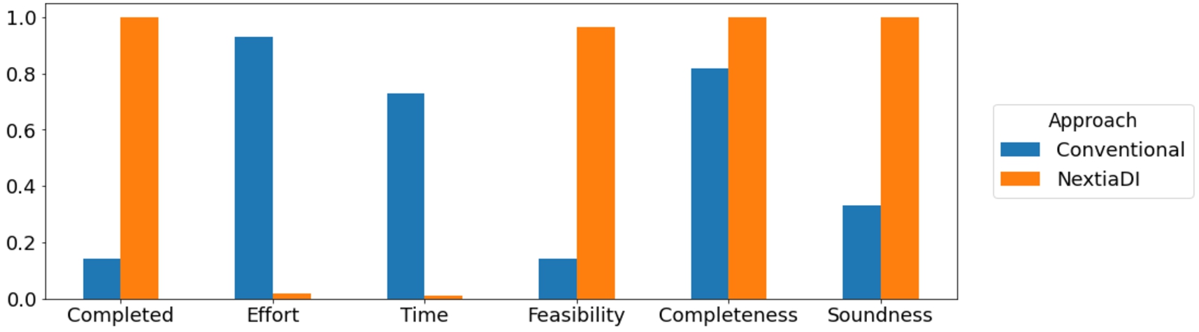
Results on generation of mappings Figure 24 shows the aggregated results for the mapping generation survey, where participants were asked to generate the mappings between the source schemata generated in step 1 and the integrated schema generated in step 2. In the conventional approach, only 37.5% of the participants managed to generate the mappings. Indeed, most participants reported a high level of effort required, while all participants generated the mappings using
Conclusion. We confirmed that
Another relevant conclusion of the experiment, raised by most of the participants, is the difficulty of the tasks at hand due to the required combined skills. In the conventional approach, they spent a considerable amount of time exploring the sources, modeling and expressing schemata and mappings in RDFS. This combined profile is difficult to find in the field of Data Science, specially, knowledge graph experts as shown in Fig. 21. This fact confirms our claim that is not feasible to make the users responsible for generating the schema integration constructs of virtual data integration systems, even for small scenarios. This can explain the low impact of such tools in industry. Fortunately, all participants believe
7.3.Scalability experiments
In order to address research question Q4, we evaluate our two technical contributions (i.e., bootstrapping and schema integration) to assess their computational complexity and runtime performance. All experiments were carried out on a Mac Intel core 2.3 GHz i5 processor with 16GB RAM and Java compiler 11.
7.3.1.Evaluation of bootstrapping
We evaluated the bootstrapping of JSON and CSV data sources by measuring the impact of the schema size. Therefore, we increase the size of the schema elements. This experiment was executed 10 times. We describe the dataset preparation and the results obtained in the following.
Dataset preparation We generated 100 datasets in JSON and CSV format. The initial JSON dataset contains a schema of 100 keys (9 objects and 91 attributes). We incrementally increased the number of schema elements by appending 50 new keys (1 object with 49 attributes) in the schema. For example, the second and third datasets will contain 150 keys (10 objects and 140 attributes) and 200 keys (11 objects and 189 attributes), respectively. For the initial CSV dataset, the schema contains 91 headers, and we incrementally appended 49 new headers.
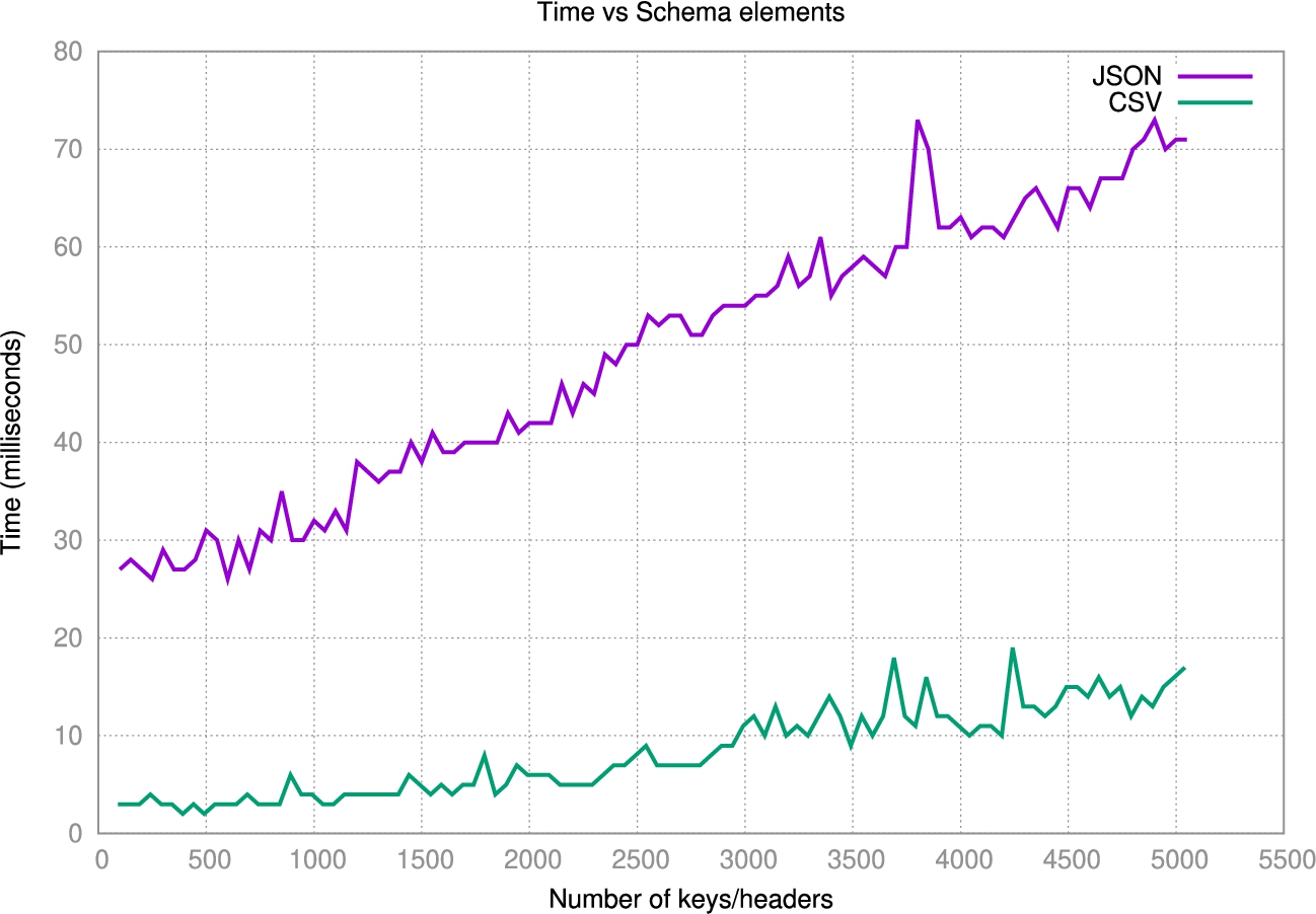
Results Figure 25 depicts the correlation between time in milliseconds and the number of keys/headers. Note that in both data sources, the time to generate a typed graph schema depends on the size of the schema. JSON bootstrapping requires more time than CSV bootstrapping, since the algorithm will parse one instance of the JSON to extract the JSON schema and apply the production rules. The initial dataset took 27 milliseconds to produce a typed graph, while the last dataset, with a schema of 108 objects and 4942 attributes, took 71 milliseconds. In contrast, CSV bootstrapping only requires the header information to produce a typed graph schema. The initial dataset took 3 milliseconds to produce the typed graph, and the last dataset, with a schema of 4942 headers, took 17 milliseconds. Overall, we can observe some peeks in the trend. However, we consider these peaks are anomalies produced due to the java garbage collector performance, since all results are constant within milliseconds. The performance obtained by the JSON and CSV shows we can rapidly bootstrap the schema in data wrangling tasks.
Fig. 25.
Performance evaluation when the number of schema elements increased.
7.3.2.Evaluation of schema integration
We evaluate the schema integration under three scenarios: (i) increasing the number of alignments in an incremental integration and (ii) integrate a constant number of alignments with a growing number of elements in the schemata and (iii) perform integration using real data.
Experiment 1 – increased alignments Here, the algorithm requires the generation of schemas and alignments that will be integrated incrementally. For the schemata, we reuse the typed graph generated by the initial JSON dataset generated in Section 7.3.1 to generate 100 typed graph schemata. All the resulting schema contain 9 classes, 90 data type properties and 1 object property. We generated the alignments between each pair of typed graph by increasing in one the number of alignments with regard to the previous pair. Therefore, the first integration generates 1 alignment and the last iteration 100 alignments. Figure 26 depicts the correlation between time in milliseconds and the number of alignments. We can observe that the time to integrate schemata depends on the number of alignments. The time to integrate one alignment took two milliseconds, while the integration of 100 alignments took 112 milliseconds. Moreover, in iteration 13, the number of integrated classes converged. Then, the remaining iteration reuses all integrated classes by applying invariant I3 from Algorithm 2. For datatype and object properties, they converged in iterations 35 and 4, respectively. Then, the remaining iterations did not create any new integrated properties. In addition, the final integrated graph contains 1000 classes, 9 integrated classes, 9000 datatype properties, 90 integrated datatype properties, 900 object properties, and 1 integrated object property. Overall, the algorithm efficiently integrates schemas incrementally.
Fig. 26.
Performance evaluation when alignments increased incrementally.
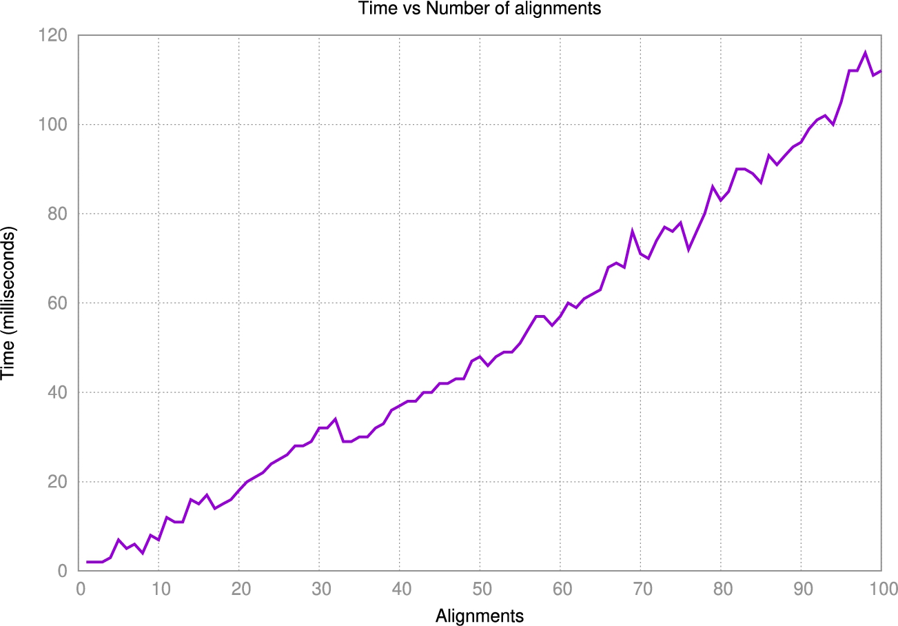
Fig. 27.
Performance evaluation when the number of schema elements increased.
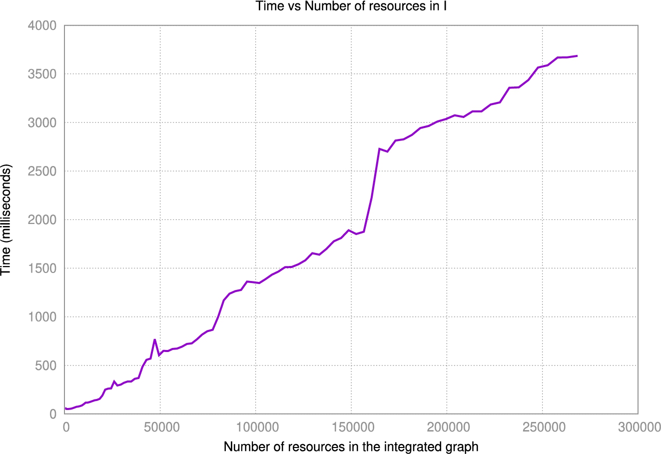
Experiment 2 – increased number of schema elements Here, we generated 100 schemas using JSON datasets where the number of elements in the schema were increased by 50 keys in each iteration. For the generation of alignments, we produced 100 alignments in each iteration since the goal is to measure the impact of the schema size in the integration. Figure 27 depicts the correlation between time in milliseconds and the total number of resources (e.g., classes and properties) in the integrated graph. We observe that the size of the integrated graph impact the time for integrating alignments. The final integrated graph contains 5950 classes, 9 integrated classes, 256500 datatype properties, 90 integrated datatype properties, 5850 object properties and 1 integrated object property. In total 268400 resources. The impact on the time due to the graph size is largely due to how Jena manages the graph in memory (the underlying triplestore used in the experiments). This demonstrates that
Experiment 3 – real data We have selected two tracks of the Ontology Alignment Evaluation Initiative: anatomy and large biomed track. The former contains the Foundational Model of Anatomy (FMA) with 2744 classes and is part of the National Cancer Institute Thesaurus (NCI) with 3304 classes. The alignments provided are 1516 class alignments. The latter contains the FMA with 78998 classes and 15 properties, and NCI with 77269 classes and 186 properties. There are 2686 class alignments for this track. This integration was performed in one step. For the anatomy track, all elements were integrated in 120 milliseconds. The final integrated graph contains 6048 classes and 1516 integrated classes. For the large biomed track, all elements were integrated in 3043 milliseconds with 156267 classes, 2686 integrated classes, 78 data type properties and 123 object properties. Overall, our integration approach is efficient when dealing with large schemas, such as the biomed track.
8.Conclusions and future work
This paper presents an approach for efficiently bootstrapping schemata of heterogeneous data sources and incrementally integrating them to facilitate the generation of schema integration constructs in virtual data integration settings. This process is specially thought to meet the requirements of data wrangling as required in Big Data scenarios: i.e., highly heterogeneous data sources and dynamic environments. As such, our proposal deal with heterogeneous data sources, follows an incremental approach to follow a pay-as-you-go integration approach and largely automates the process. Relevantly, our approach is not specific for a given system and it generates system-agnostic metadata that can be later used to generate the specific constructs of the most relevant virtual data integration systems. Last but not least, we have presented
This work opens many interesting research lines from it. For example, how to generalize the current approach to integrate complex semantic relationships between schemas (beyond one-to-one mappings) or develop a hybrid approach that, once the integrated schema is generated in a bottom-up approach, it allows the user to enrich the automatically generated outputs in a top-down approach. The ultimate question we would like to address is how to use these techniques to suggest refactoring techniques over the underlying data sources to facilitate their alignment and integration.
Notes
4 In the ancient Nahuatl language, the term nextia means to get something out or put something together.
5 See more details at https://www.essi.upc.edu/dtim/nextiadi/.
8 Note that virtual data integration systems just consider schema integration and disregard record linkage and data fusion. Thus, in the original framework it talks about data integration, which is used as a synonym of schema integration.
15 The notebooks and all experiments data are available on the companion website of this paper.
Acknowledgements
This work was partly supported by the DOGO4ML project, funded by the Spanish Ministerio de Ciencia e Innovación under project PID2020-117191RB-I00, and D3M project, funded by the Spanish Agencia Estatal de Investigación (AEI) under project PDC2021-121195-I00. Javier Flores is supported by contract 2020-DI-027 of the Industrial Doctorate Program of the Government of Catalonia and Consejo Nacional de Ciencia y Tecnología (CONACYT, Mexico). Sergi Nadal is partly supported by the Spanish Ministerio de Ciencia e Innovación, as well as the European Union – NextGenerationEU, under project FJC2020-045809-I.
Appendices
Appendix A.
Appendix A.JSON metamodel constraints
In this appendix, we present the constraints considered for the metamodel we adopt to represent the schemata of JSON datasets (i.e.,
IS-A relationships and constraints on generalizations Rule 1 restricts instances of  to be instances of either
  ,
,  or
or  . Then, Rules 2, 3, and 4 constrain that for any of such subclass instances, the instantiation of the superclass
  also exists in G. Finally, Rules 5, 6 and 7 determine that the subclasses of
  are disjoint.
Referential integrity constraints Rule 8 indicates that an edge labeled with  will connect instances of either
  and
and  , or instances of
  and
and  . Similarly, Rule 9 applies the same strategy to connect instances of
  and
and  using edges labeled
  .
.
Cardinality constraints Rule 10 states that an instance of  has a single instance of
  as root. Then, Rule 11 models a many-to-one relationship between instances of
  and
and  .
.
Appendix B.
Appendix B.RDFS metamodel constraints
In this appendix, we present the constraints considered for the fragment of RDFS that we consider in this paper (i.e.,
IS-A relationships and constraints on generalizations Rule 12 restricts instances of  to be instances of either
  or
or  . Then, Rules 13 and 14, constrain that for any of such subclass instances, the instantiation of the superclass
  also exists in G. Next, Rule 15 denote that instances of
  are also instances of
  .
.
Referential integrity constraints Rule 16 indicates that the  of an instance of
  is an instance of
  . Similarly, Rule 17, constraints that the
  of instances of
  are also instances of
  .
.
B.1.Schema integration constraints
Here we present the constraints for the RDFS metamodel extension we consider to support the annotated integration process depicted in Section 5.
IS-A relationships Rule 18 states that any instance of  is also an instance of
  . Similarly, Rule 19, denotes that any instance of
  is also an instance of
  .
.
Referential integrity constraints Rule 20 denotes that the  of a
of a  instance is an
  .
.
References
[1] | D. Abadi, A. Ailamaki, D.G. Andersen, P. Bailis, M. Balazinska, P.A. Bernstein, P.A. Boncz, S. Chaudhuri, A. Cheung, A. Doan, L. Dong, M.J. Franklin, J. Freire, A.Y. Halevy, J.M. Hellerstein, S. Idreos, D. Kossmann, T. Kraska, S. Krishnamurthy, V. Markl, S. Melnik, T. Milo, C. Mohan, T. Neumann, B.C. Ooi, F. Ozcan, J.M. Patel, A. Pavlo, R.A. Popa, R. Ramakrishnan, C. Ré, M. Stonebraker and D. Suciu, The Seattle report on database research, Commun. ACM 65: (8) ((2022) ), 72–79. doi:10.1145/3524284. |
[2] | K.M. Albarrak and E.H. Sibley, A survey of methods that transform data models into ontology models, in: IRI, IEEE Systems, Man, and Cybernetics Society, (2011) , pp. 58–65. |
[3] | P. Atzeni, P. Cappellari, R. Torlone, P.A. Bernstein and G. Gianforme, Model-independent schema translation, VLDB J. 17: (6) ((2008) ), 1347–1370. doi:10.1007/s00778-008-0105-2. |
[4] | S. Babalou, E. Grygorova and B. König-Ries, What to do when the users of an ontology merging system want the impossible? Towards determining compatibility of generic merge requirements, in: EKAW, Lecture Notes in Computer Science, Vol. 12387: , Springer, (2020) . |
[5] | S. Babalou and B. König-Ries, Towards building knowledge by merging multiple ontologies with CoMerger: A partitioning-based approach, 2020, CoRR arXiv:2005.02659. |
[6] | I. Bedini, C.J. Matheus, P.F. Patel-Schneider, A. Boran and B. Nguyen, Transforming XML schema to OWL using patterns, in: ICSC, IEEE Computer Society, (2011) , pp. 102–109. |
[7] | P.A. Bernstein, J. Madhavan and E. Rahm, Generic schema matching, ten years later, Proc. VLDB Endow. 4: (11) ((2011) ), 695–701. doi:10.14778/3402707.3402710. |
[8] | C. Bizer and R. Cyganiak, D2r server-publishing relational databases on the semantic web, in: Poster at the 5th International Semantic Web Conference, Vol. 175: , (2006) . |
[9] | A. Bonifati, G.H.L. Fletcher, H. Voigt and N. Yakovets, Querying Graphs, Synthesis Lectures on Data Management, Morgan & Claypool Publishers, (2018) . |
[10] | M. Buron, F. Goasdoué, I. Manolescu and M. Mugnier, Obi-Wan: Ontology-based RDF integration of heterogeneous data, Proc. VLDB Endow. 13: (12) ((2020) ), 2933–2936. doi:10.14778/3415478.3415512. |
[11] | D. Calvanese, B. Cogrel, S. Komla-Ebri, R. Kontchakov, D. Lanti, M. Rezk, M. Rodriguez-Muro and G. Xiao, Ontop: Answering SPARQL queries over relational databases, Semantic Web 8: (3) ((2017) ), 471–487. doi:10.3233/SW-160217. |
[12] | C. Civili, M. Console, G.D. Giacomo, D. Lembo, M. Lenzerini, L. Lepore, R. Mancini, A. Poggi, R. Rosati, M. Ruzzi, V. Santarelli and D.F. Savo, MASTRO STUDIO: Managing ontology-based data access applications, Proc. VLDB Endow. 6: (12) ((2013) ), 1314–1317. doi:10.14778/2536274.2536304. |
[13] | M. da Conceição Moraes Batista and A.C. Salgado, Information quality measurement in data integration schemas, in: QDB, (2007) , pp. 61–72. |
[14] | L.F. de Medeiros, F. Priyatna and Ó. Corcho, MIRROR: Automatic R2RML mapping generation from relational databases, in: ICWE, Lecture Notes in Computer Science, Vol. 9114: , Springer, (2015) , pp. 326–343. |
[15] | X.L. Dong and D. Srivastava, Big Data Integration, Synthesis Lectures on Data Management, Morgan & Claypool Publishers, (2015) . |
[16] | D. Dou, D.V. McDermott and P. Qi, Ontology translation on the Semantic Web, J. Data Semant. 2: ((2005) ), 35–57. doi:10.1007/978-3-540-30567-5_2. |
[17] | K.M. Endris, P.D. Rohde, M. Vidal and S. Auer, Ontario: Federated query processing against a semantic data lake, in: DEXA (1), Lecture Notes in Computer Science, Vol. 11706: , Springer, (2019) , pp. 379–395. |
[18] | J. Flores, S. Nadal and O. Romero, Towards scalable data discovery, in: EDBT, OpenProceedings.org, (2021) , pp. 433–438. |
[19] | M. Giese, A. Soylu, G. Vega-Gorgojo, A. Waaler, P. Haase, E. Jiménez-Ruiz, D. Lanti, M. Rezk, G. Xiao, Ö.L. Özçep and R. Rosati, Optique: Zooming in on Big Data, Computer 48: (3) ((2015) ), 60–67. doi:10.1109/MC.2015.82. |
[20] | B. Golshan, A.Y. Halevy, G.A. Mihaila and W. Tan, Data integration: After the teenage years, in: PODS, ACM, (2017) , pp. 101–106. |
[21] | W.A. Günther, M.H.R. Mehrizi, M. Huysman and F. Feldberg, Debating big data: A literature review on realizing value from big data, J. Strateg. Inf. Syst. 26: (3) ((2017) ), 191–209. doi:10.1016/j.jsis.2017.07.003. |
[22] | L.M. Haas, Beauty and the beast: The theory and practice of information integration, in: ICDT, Lecture Notes in Computer Science, Vol. 4353: , Springer, (2007) , pp. 28–43. |
[23] | M. Hacherouf, S.N. Bahloul and C. Cruz, Transforming XML documents to OWL ontologies: A survey, J. Inf. Sci. 41: (2) ((2015) ), 242–259. doi:10.1177/0165551514565972. |
[24] | G. Haesendonck, W. Maroy, P. Heyvaert, R. Verborgh and A. Dimou, Parallel RDF generation from heterogeneous big data, in: SBD@SIGMOD, ACM, (2019) , pp. 1:1–1:6. |
[25] | A. Halevy, M. Franklin and D. Maier, Principles of dataspace systems, in: Proceedings of the 25th ACM SIGMOD-SIGACT-SIGART Symposium on Principles of Database Systems, ACM, (2006) , pp. 1–9. |
[26] | A.Y. Halevy, A. Rajaraman and J.J. Ordille, Data integration: The teenage years, in: VLDB, ACM, (2006) , pp. 9–16. |
[27] | B.E. Idrissi, S. Baïna and K. Baïna, Automatic generation of ontology from data models: A practical evaluation of existing approaches, in: RCIS, IEEE, (2013) , pp. 1–12. |
[28] | E. Iglesias, S. Jozashoori, D. Chaves-Fraga, D. Collarana and M. Vidal, SDM-RDFizer: An RML interpreter for the efficient creation of RDF knowledge graphs, in: CIKM, ACM, (2020) , pp. 3039–3046. |
[29] | J.L.C. Izquierdo and J. Cabot, Discovering implicit schemas in JSON data, in: ICWE, Lecture Notes in Computer Science, Vol. 7977: , Springer, (2013) , pp. 68–83. |
[30] | E. Jiménez-Ruiz and B.C. Grau, LogMap: Logic-based and scalable ontology matching, in: ISWC (1), Lecture Notes in Computer Science, Vol. 7031: , Springer, (2011) , pp. 273–288. |
[31] | E. Jiménez-Ruiz, E. Kharlamov, D. Zheleznyakov, I. Horrocks, C. Pinkel, M.G. Skjæveland, E. Thorstensen and J. Mora, BootOX: Practical mapping of RDBs to OWL 2, in: ISWC (2), Lecture Notes in Computer Science, Vol. 9367: , Springer, (2015) , pp. 113–132. |
[32] | P. Jovanovic, S. Nadal, O. Romero, A. Abelló and B. Bilalli, Quarry: A user-centered big data integration platform, Inf. Syst. Frontiers 23: (1) ((2021) ), 9–33. doi:10.1007/s10796-020-10001-y. |
[33] | S. Kandel, J. Heer, C. Plaisant, J. Kennedy, F. van Ham, N.H. Riche, C.E. Weaver, B. Lee, D. Brodbeck and P. Buono, Research directions in data wrangling: Visualizations and transformations for usable and credible data, Inf. Vis. 10: (4) ((2011) ), 271–288. doi:10.1177/1473871611415994. |
[34] | S. Kandel, A. Paepcke, J.M. Hellerstein and J. Heer, Enterprise data analysis and visualization: An interview study, IEEE Trans. Vis. Comput. Graph. 18: (12) ((2012) ), 2917–2926. doi:10.1109/TVCG.2012.219. |
[35] | E. Kharlamov, S. Brandt, M. Giese, E. Jiménez-Ruiz, S. Lamparter, C. Neuenstadt, Ö.L. Özçep, C. Pinkel, A. Soylu, D. Zheleznyakov, M. Roshchin, S. Watson and I. Horrocks, Semantic access to siemens streaming data: The optique way, in: ISWC (Posters & Demos), CEUR Workshop Proceedings, Vol. 1486: , CEUR-WS.org, (2015) . |
[36] | C.A. Knoblock, P.A. Szekely, J.L. Ambite, A. Goel, S. Gupta, K. Lerman, M. Muslea, M. Taheriyan and P. Mallick, Semi-automatically mapping structured sources into the Semantic Web, in: ESWC, Lecture Notes in Computer Science, Vol. 7295: , Springer, (2012) . |
[37] | M. Lenzerini, Data integration: A theoretical perspective, in: PODS, ACM, (2002) , pp. 233–246. |
[38] | M.N. Mami, D. Graux, S. Scerri, H. Jabeen, S. Auer and J. Lehmann, Squerall: Virtual ontology-based access to heterogeneous and large data sources, in: ISWC (2), Lecture Notes in Computer Science, Vol. 11779: , Springer, (2019) , pp. 229–245. |
[39] | D.L. McGuinness, R. Fikes, J. Rice and S. Wilder, The chimaera ontology environment, in: AAAI/IAAI, AAAI Press/The MIT Press, (2000) , pp. 1123–1124. |
[40] | P. Mitra, G. Wiederhold and S. Decker, A scalable framework for the interoperation of information sources, in: SWWS, (2001) , pp. 317–329. |
[41] | S. Nadal, A. Abelló, O. Romero, S. Vansummeren and P. Vassiliadis, MDM: Governing evolution in big data ecosystems, in: EDBT, OpenProceedings.org, (2018) , pp. 682–685. |
[42] | S. Nadal, A. Abello, O. Romero, S. Vansummeren and P. Vassiliadis, Graph-driven federated data management, IEEE Transactions on Knowledge and Data Engineering 35: (1) ((2023) ), 509–520. doi:10.1109/TKDE.2021.3077044. |
[43] | S. Nadal, K. Rabbani, O. Romero and S. Tadesse, ODIN: A dataspace management system, in: ISWC (Satellites), CEUR Workshop Proceedings, Vol. 2456: , CEUR-WS.org, (2019) , pp. 185–188. |
[44] | N.F. Noy and M.A. Musen, PROMPT: Algorithm and tool for automated ontology merging and alignment, in: AAAI/IAAI, AAAI Press/The MIT Press, (2000) , pp. 450–455. |
[45] | I. Osman, S.B. Yahia and G. Diallo, Ontology integration: Approaches and challenging issues, Inf. Fusion 71: ((2021) ), 38–63. doi:10.1016/j.inffus.2021.01.007. |
[46] | N.W. Paton, K. Belhajjame, S.M. Embury, A.A.A. Fernandes and R. Maskat, Pay-as-you-go data integration: Experiences and recurring themes, in: SOFSEM, Lecture Notes in Computer Science, Vol. 9587: , Springer, (2016) , pp. 81–92. |
[47] | P. Pereira, J. Cunha and J.P. Fernandes, On understanding data scientists, in: VL/HCC, IEEE, (2020) , pp. 1–5. |
[48] | C. Pinkel, C. Binnig, E. Jiménez-Ruiz, E. Kharlamov, A. Nikolov, A. Schwarte, C. Heupel and T. Kraska, IncMap: A journey towards ontology-based data integration, in: BTW, LNI, Vols P-265: , GI, (2017) , pp. 145–164. |
[49] | F. Priyatna, R. Alonso-Calvo, S. Paraiso-Medina, G. Padron-Sanchez and Ó. Corcho, R2RML-based access and querying to relational clinical data with morph-RDB, in: SWAT4LS, CEUR Workshop Proceedings, Vol. 1546: , CEUR-WS.org, (2015) , pp. 142–151. |
[50] | F. Priyatna, Ó. Corcho and J.F. Sequeda, Formalisation and experiences of R2RML-based SPARQL to SQL query translation using morph, in: WWW, ACM, (2014) , pp. 479–490. |
[51] | S. Raunich and E. Rahm, Target-driven merging of taxonomies with atom, Inf. Syst. 42: ((2014) ), 1–14. doi:10.1016/j.is.2013.11.001. |
[52] | J.F. Sequeda, S.H. Tirmizi, Ó. Corcho and D.P. Miranker, Survey of directly mapping SQL databases to the Semantic Web, Knowl. Eng. Rev. 26: (4) ((2011) ), 445–486. doi:10.1017/S0269888911000208. |
[53] | M. Solanki, C. Mader, H. Nagy, M. Mückstein, M. Hanfi, R. David and A. Koller, Ontology-driven unified governance in software engineering: The PoolParty case study, in: ESWC (2), Lecture Notes in Computer Science, Vol. 10250: , (2017) , pp. 109–124. |
[54] | M. Stonebraker and I.F. Ilyas, Data integration: The current status and the way forward, IEEE Data Eng. Bull. 41: (2) ((2018) ), 3–9. |
[55] | G. Stumme and A. Maedche, FCA-MERGE: Bottom-up merging of ontologies, in: IJCAI, Morgan Kaufmann, (2001) , pp. 225–234. |
[56] | P.T.T. Thuy, Y. Lee and S. Lee, DTD2OWL: Automatic transforming XML documents into OWL ontology, in: ICIS, ACM International Conference Proceeding Series, Vol. 403: , ACM, (2009) , pp. 125–131. doi:10.1145/1655925.1655949. |
[57] | C. Tsinaraki and S. Christodoulakis, XS2OWL: A formal model and a system for enabling XML schema applications to interoperate with OWL-DL domain knowledge and Semantic Web tools, in: DELOS, Lecture Notes in Computer Science, Vol. 4877: , Springer, (2007) . |
[58] | B. Vidé, J. Marty, F. Ravat and M. Chevalier, Designing a business view of enterprise data: An approach based on a decentralised enterprise knowledge graph, in: IDEAS, ACM, (2021) , pp. 184–193. |
[59] | G. Xiao, D. Calvanese, R. Kontchakov, D. Lembo, A. Poggi, R. Rosati and M. Zakharyaschev, Ontology-based data access: A survey, in: IJCAI, ijcai.org, (2018) , pp. 5511–5519. |


