
Characteristic sets profile features: Estimation and application to SPARQL query planning
Abstract
RDF dataset profiling is the task of extracting a formal representation of a dataset’s features. Such features may cover various aspects of the RDF dataset ranging from information on licensing and provenance to statistical descriptors of the data distribution and its semantics. In this work, we focus on the characteristics sets profile features that capture both structural and semantic information of an RDF dataset, making them a valuable resource for different downstream applications. While previous research demonstrated the benefits of characteristic sets in centralized and federated query processing, access to these fine-grained statistics is taken for granted. However, especially in federated query processing, computing this profile feature is challenging as it can be difficult and/or costly to access and process the entire data from all federation members. We address this shortcoming by introducing the concept of a profile feature estimation and propose a sampling-based approach to generate estimations for the characteristic sets profile feature. In addition, we showcase the applicability of these feature estimations in federated querying by proposing a query planning approach that is specifically designed to leverage these feature estimations. In our first experimental study, we intrinsically evaluate our approach on the representativeness of the feature estimation. The results show that even small samples of just
1.Introduction
In recent years, the amount of information published as Linked Open Data has steadily increased as new RDF datasets are published and existing datasets are growing.11 Simultaneously, Semantic Web technologies are more and more used in companies to integrate data from heterogeneous sources using Knowledge Graphs and Semantic Data Lakes [22,30,31]. In order to support applications that leverage these large corpora of semantic data, we require means to extract high-level information on the content, the quality, and the structure of the data provided by these sources. To this end, a variety of approaches have been proposed to summarize semantic graphs [9], assess their quality [43] and extract various features in dataset profiles [13]. Similar to the field of databases, where “Data profiling refers to the activity of creating small but informative summaries of a database” [19], RDF dataset profiling aims to formally represent a set of features of an RDF dataset to aid downstream tasks [12]. RDF dataset profiles typically consist of several profile features that capture information that ranges from licensing, provenance to statistical characteristics of the dataset [13]. The cost to acquire statistical features depend on their granularity as well as the size of and the means to access the RDF dataset. Dataset profiling techniques typically assume local access to the entire datasets such that the features can be computed more efficiently. Upon creation, RDF dataset profiles support applications such as entity linking, entity retrieval, distributed search and (federated) query processing [13]. In particular, centralized and federated query engines rely on fine-grained dataset profiles to obtain efficient query plans [4,10,15,26,27,32,35,36]. For instance, characteristic sets are often used to estimate join cardinalities in query plan optimization [25–27,32].
In this work, we focus on the Characteristic Sets Profile Feature (CSPF) [17], which is a statistical feature of RDF datasets that includes the characteristic sets, their occurrence distribution, and the multiplicity of their predicates. We focus on this particular profile features as an informative statistical characterization of RDF datasets due to the following reasons. First, CSPFs implicitly captures structural features of the data, such as the mean out-degree, distinct number of subjects, and the set of predicates including their counts. Second, characteristic sets implicitly reflect the schema of an RDF dataset as they capture semantic information on its entities. Finally, CSPFs are well suited to be leveraged by (decentralized) query planning approaches for cardinality estimations and other downstream tasks as they provide insights into the predicate co-occurrence. While the CSPFs provide rich information that is beneficial for various applications, obtaining the profile feature can be a challenging task. For instance, the federated query planning approach Odyssey [26] exploits information on the characteristic sets and how they are linked across datasets to estimate intermediate results when optimizing query plans. Yet, especially in federated query processing, it can be difficult and/or costly to access the entire RDF datasets of all members in the federation and, subsequently, compute these fine-grained statistics. First, data dumps are not always available in federated querying as data publisher may choose different Linked Data Fragments (LDFs) to publish their data [40]. For example, the datasets may only be partially accessed via SPARQL endpoints or Triple Pattern Fragment servers. Moreover, in the case of public resources, the statistics need to be obtained while respecting the fair use policies of the publisher [39]. Second, to build the characteristic sets for an RDF dataset requires scanning the entire dataset. This computational effort can be an additional restriction, especially for very large and evolving datasets, such as DBpedia22 or Wikidata33 with more than a billion triples that are updated frequently
Addressing these limitations, we propose an approach that estimates accurate statistical profile features based on characteristic sets and that relies only on a small sample of the original dataset. Our sample-based approach alleviates the necessity of having access to the entire dataset and also reduces the cost of computing the profile feature. Given an RDF dataset, our approach employs an entity-enteric sampling method and computes the characteristic sets of the entities to build the CSPF of the sample. Then, we apply a projection function to extrapolate the statistics observed in the sample to estimate the original dataset’s CSPF. As the statistics of the characteristic sets are sensitive to the structure of the datasets and the sample, this extrapolation step can be challenging. Take for example the following characteristic sets
Table 1
LinkedMDB: Example characteristic sets
| Characteristic Set | ||
| 9838 | ||
| 5 | ||
| 697 |
We observe that the characteristic set
RQ 1 Which steps are sufficient for accurately estimating RDF dataset profile features? First, we want to investigate how we can estimate profile features without requiring access to the entire dataset. In particular, we study which sampling methods are suitable to obtain a representative sample for the specific characteristic sets profile feature. Based on samples, we investigate how the information captured in the sample can be extrapolated to the original dataset. The goal of this research question is, therefore, to understand the impact of different sampling methods, sample sizes, and extrapolation techniques on the profile feature estimation.
RQ 2 How can we assess the effectiveness of estimated profile features? Given the original profile feature and an estimation, we need means to assess the accuracy of the estimation. As we focus on the characteristic sets profile features that capture various characteristics of the dataset, we investigate how the representativeness of an estimation with respect to those characteristics can be measured. Moreover, with this question, we also want to understand which characteristics are more difficult to estimate and how the structure of the original dataset impacts the estimations.
RQ 3 How can we leverage estimated profile features to support downstream applications such as federated query processing? This question aims to investigate how estimated profile features still support applications that rely on these features. As we focus on the characteristic sets profile feature, we consider applications that leverage this information and where the computation of the complete statistics may not be feasible. Therefore, we investigate how a federated query planning approach can leverage the estimated profile features. Specifically, we study how source selection, query decomposition, and join ordering is affected by different estimations. Finally, we want to understand to which extent the effectiveness of the estimation (c.f. ) is reflected in the performance of the query plans.
Contributions This paper builds on a previous work of ours [17], which focuses on a sampling-based approach for estimating characteristic sets for RDF dataset profiles. We extend this work regarding two major aspects. First, we expand our experimental evaluation about CSPF estimations by studying additional datasets and providing a more fine-grained analysis of the results. Second, we address a central aspect of the profile feature estimations, which is their application in downstream tasks. Particularly, we propose a novel federated query planning approach based on the profile feature estimations. Finally, we evaluate this approach in an experimental study. In summary, the novel contributions of this work are as follows.
C 1 An extensive experimental study of our Characteristic Sets Profile Feature estimation approach on eight new datasets,
C 2 a fine-grained analysis of the results to understand the effectiveness of our CSPF estimation approach and its components,
C 3 a new estimations-based query planner to showcase the application of the estimations in federated query processing,
C 4 an experimental study of our query planner on the well-known FedBench benchmark, and
C 5 a detailed evaluation of the results to understand the benefits and limitations of the query planner.
Structure of this paper The remainder of this work is organized as follows. In Section 2, we introduce RDF dataset profiling and present our problem definition for estimating profile features. We define characteristic sets profile features and present our sampling-based approach to estimate them in Section 3. In Section 4, we present an application of the estimated profile features in federated query planning. We evaluate our profile feature estimation and estimation-based query approaches in Section 5. Related work on statistical profiling, graph sampling, and federated query processing is discussed in Section 6. Finally, we conclude our work with remarks on future work in Section 7.
2.RDF dataset profiling
The Resource Description Framework (RDF) is a graph-based data model. The atomic elements in RDF are triples, which are statements represented as 3-tuple of RDF terms:
2.1.Profile features
RDF datasets are summarized in RDF dataset profiles that consist of profile features describing the characteristics and entities of the dataset. In the area of traditional relational database theory, a statistical profile is defined as a “complex object composed of quantitative descriptors” that “summarizes the instances of a database” [23]. These quantitative descriptors can cover different characteristics of the instances, for example:
– central tendency (e.g., mean),
– dispersion, (e.g., coefficient of variation),
– size (e.g., number of instances), and
– frequency distribution (e.g., uniformity).
The specific characteristics covered in such profiles depend on the downstream application, for example, the statistical features required by a query optimizer that uses the profile to devise efficient query plans. Similar to relational databases, statistic profiles are also commonly used for a variety of applications in the realm of RDF datasets. These applications range from centralized RDF data management solutions [28] and RDF graph compression [14] to query optimization for both centralized and federated query processing [16,24,26]. For instance, a common application of such statistical profiles in query optimization is the estimation of join cardinalities for subqueries.
The terminology for such statistical profiles varies according to their application [9,13,43]. In this work, we follow the terminology introduced by Ellefi et al. [13]: An RDF dataset profile is a formal representation of a set of dataset profile features. Moreover, we focus on statistical profile features and define them as follows.
Definition 2.1
Definition 2.1(Profile Feature [17]).
Given an RDF graph G, a profile feature
As previously mentioned, computing these profile features can be challenging because accessing and processing the entire datasets is difficult and/or costly. Therefore, we investigate profile feature estimation without requiring access to the complete RDF graph.
2.2.Profile feature estimation
Addressing the limitation of requiring access to the entire RDF dataset for computing statistical profile features, we propose the concept of Profile Feature Estimation. Profile feature estimations aim to estimate a statistical profile features of RDF datasets using a subset of the data only. The goal is to generate a profile feature estimation that is as similar as possible to the original profile feature while requiring access to a subset of the dataset only. In particular, we propose an approach that relies on a sample from the original RDF graph in combination with a projection function to extrapolate the true profile feature. Consequently, we define a profile feature estimation as follows.
Definition 2.2
Definition 2.2(Profile Feature Estimation [17]).
Given an RDF graph G, a projection function ϕ, a subgraph
In an ideal situation, the estimated profile feature is identical to the true original profile feature (computed over the complete RDF graph). However, the profile feature to be estimated and the properties of both the subgraph H and the projection function ϕ may affect the differences between the true and the estimated feature. For example, given a larger subgraph, the estimation might be more accurate than for a smaller subgraph, as the larger subgraph potentially covers more characteristics of the original graph. The problem is finding an estimation for the profile feature which maximizes the similarity to the profile feature of the original RDF graph. To this aim, we introduce the concept of a similarity function δ that maps two profile features to a similarity value. The profile feature estimation problem is given as finding a profile feature estimation that maximizes the similarity to the original profile feature.
Definition 2.3
Definition 2.3(Profile Feature Estimation Problem [17]).
Given an RDF graph G and a profile feature
In order to maximize the similarity, the sampling algorithm for obtaining H and the projection function ϕ need to be chosen appropriately. The particular method to measure the similarity δ depends on the actual profile feature to be estimated with potentially several similarity functions for the same profile feature. Take for example a profile feature
3.Characteristic sets profile feature estimation
We now present our sampling-based approach to estimate profile features based on the characteristics sets of RDF graphs. In this section, we first introduce the concept of characteristics sets and define the corresponding Characteristic Sets Profile Feature. Thereafter, we present our approach that combines RDF graph sampling with projection functions to estimate the Characteristic Sets Profile Feature. Finally, we propose structural and statistical similarity measures to assess the representativeness of these estimations.
3.1.Characteristic sets profile feature
The concept of characteristic sets for RDF graphs was introduced by Neumann et al. [27]. In their work, the authors used characteristics sets for query planning as they capture the co-occurrences of predicates in RDF graphs. The idea of characteristic sets is describing semantically similar entities by grouping them according to the set of predicates the entities share. Furthermore, the number of entities in each group are counted as well as the average usage of their predicates. As a result, the characteristic sets capture both statistical information on the data distribution as well as semantic information on the entities in an RDF graph.
Definition 3.1
Definition 3.1(Characteristic Sets [27]).
The characteristic set of an entity s in an RDF graph G is given by:
In an RDF graph, the statistical information determined for the characteristic sets typically includes the number of occurrences (count) of a given characteristic set as well as the multiplicities of the predicates within each characteristic set. These statistics are used in both centralized triple stores and federated query engines because they allow to determine exact join cardinalities for specific Distinct queries and to compute cardinality estimations for non-distinct queries [16,24,26,27]. Similar to Neumann et al. [27], we define the number of occurrences
In addition, in this work, we focus on the occurrences of predicates in characteristic sets by considering their mean multiplicity. The mean multiplicity
In other words, for a given characteristic set, the multiplicity measures how often each predicate occurs on average. Combining the count and mean multiplicity statistics of a characteristic set, we can compute the number of triples that are covered by it. The relative coverage
For example, consider the characteristic set
–
–
–
–
The statistics indicate that 9838 entities in the LinkedMDB graph belong to
Finally, we introduce the notion of exclusive characteristic sets. An exclusive characteristic set occurs only once in an RDF graph and is defined as the following.
Definition 3.2
Definition 3.2(Exclusive Characteristic Sets [17]).
Given the characteristic sets
For example, in the LinkedMDB graph there exists only one entity with the predicates lmdb:relatedBook and lmdb:language. Therefore, the characteristics set
Based on these definitions, the statistical aspects of characteristics sets can be combined to formally define the characteristic sets profile feature (CSPF) as follows.
Definition 3.3
Definition 3.3(Characteristic Sets Profile Feature (CSPF) [17]).
Given a RDF graph G, the characteristic sets profile feature
We now present the individual steps of our approach for estimating the CSPF of a given RDF graph.
Overview of the approach We propose a sampling-based approach that is shown in Fig. 1. Given a graph G, the approach generates a sample
Fig. 1.
Overview of the approach: a sample H is taken from the original graph G. The profile feature
![Overview of the approach: a sample H is taken from the original graph G. The profile feature F(G) is created and projected to obtain the profile feature estimation ϕ(F(H))=Fˆ(G)… (based on [17]).](https://ip.ios.semcs.net:443/media/sw/2023/14-3/sw-14-3-sw222903/sw-14-sw222903-g001.jpg)
3.2.Graph sampling
The first step of our approach is obtaining a representative sample of the original RDF graph that provides a suitable foundation for estimating the profile feature. Before collecting data from a population in a sample, an appropriate sampling method needs to be chosen. Accordingly, we focus on sampling methods suitable for estimating the CSPF. Since characteristic sets capture the attributes of the entities in an RDF graph, we focus on entity-centered sampling methods in the following. Each entity (i.e., subject) is associated with exactly one characteristic set, thus, we define the population to be sampled from as the set of entities in the given graph:
Unweighted sampling The unweighted sampling method selects
Weighted sampling The weighted sampling method is a biased sampling method, where the probability of an entity to be part of the sample is proportional to its out-degree. As a result, the more central an entity is in the graph with respect to its out-degree centrality [29], the more likely it is part of the sample. In this way, entities that appear in many triples of the graph in the subject position, have a higher probability of being selected. The out-degree of each entity e given by
Hybrid sampling The hybrid sampling method combines the previous two sampling methods. From the original graph,
The β parameter allows for favoring either the weighted or the unweighted method.
3.3.Profile feature creation
After obtaining a subgraph H using a sampling method, the characteristic sets profile feature
3.4.Profile feature projection
Given the profile feature
We now present two classes of projection functions for the count values of the characteristic sets in the sample. The first class, which we denote basic projection functions, only relies on information contained within the sample and the size of the original graph. The second class, which we denote as statistics-enhanced projection functions also relies on high-level information on the original dataset in addition to the information contained in the sample.
Basic projection function The basic projection function extrapolates the count values for the given characteristic sets profile feature
The assumption of the basic projection function is that the characteristic sets observed in a sample occur proportionally more often in the original graph. However, as exemplified in the introduction, the distributions of the counts may be potentially skewed which is not considered by this projection function. Moreover, this function neglects the fact that some characteristics sets might not have been sampled and merely distributes the proportional counts across the characteristic sets in the sample. As a result, it is likely that the counts for the characteristic sets is overestimated, especially if just a small portion of characteristics sets from the original graph are captured. To address this shortcoming, we introduce two statistic-enhanced projection functions that leverage high-level information to reduce the probability of overestimating the counts.
Statistics-enhanced projection functions The second class of projection functions incorporates additional high-level information about the original graph. In particular, we consider the number of triples per predicate in the original graph as this high-level statistic. The rationale for this particular statistic is that it potentially yields a good trade-off between the effort to obtain the statistic and the benefit it provides for the projection function. The number of triples for predicate
The first statistic-enhanced projection function,
The idea of this projection function is that the predicate occurrence statistics of the original graph allows for limiting the estimated counts for characteristic sets containing that predicate. If a predicate
The projection function
In contrast to
Concluding this section on the projection functions, we want to note that further functions may be applied to potentially improve the estimation of the profile feature. For example, the characteristic sets sizes or additional statistics about the predicate distribution in the sample could be considered. However, we chose not to include them since they are likely to just produce accurate estimation under certain conditions and, therefore, do not generalize well for other datasets. Moreover, further improvements in the estimations do not necessarily imply the same improvements in the downstream applications that use the feature estimations.
3.5.Sampling RDF graphs in practice
The presented sampling approaches define the process for selecting entities to be sampled from the original graph but they do not encode how the samples are generated in practice. The implementation of the sampling approaches depends on the access methods to the given RDF graph. In the case of centralized RDF graphs, the sampling approach has access to the entire dataset and could potentially exploit existing data structures (e.g., indices) to efficiently access the entities in the graph. However, in decentralized scenarios as federations, the sampling methods have only access to parts of the RDF graphs and their implementation depends on the expressivity, capabilities, and configuration of the access interfaces. While it is out of the scope of this work to present specific implementations for each access interface, in the following, we provide insights into the considerations when implementing these sampling methods over remote SPARQL endpoints and Triple Pattern Fragments (TPF) servers.
SPARQL endpoints The expressivity of endpoints allows for selecting the entities to be sampled and then obtaining the subgraph induced by those entities.
The unweighted sampling method can be implemented over a SPARQL endpoint as follows. (i) Query all unique subjects (i.e., with Select and Distinct). If the number of entities exceeds the number of answers allowed per response, the implementation can retrieve all the entities by ‘paginating’ the results by ordering them with Order By and using Limit and Offset. (ii) Select
In the weighted sampling method, the out-degree of an entity determines its probability to be sampled. To avoid computing the out-degree for each entity, it is possible to implement a simple heuristic that relies on the following assumption: The higher an entity’s out-degree, the more triples with it in the subject positions are present in the graph. Therefore, to obtain a weighted sample, the approach can randomly select triples from the graph and obtain the subjects of those triples. This can be achieved in endpoints using a query that matches any triple in the graph, a Limit of 1, and a random Offset value between 0 and the size of the graph
Finally, after the entities have been selected, the induced subgraph of the entities can be obtained using either a Construct query or a Select query. That is, all triples where the entities are in the subject position will be constructed. This can be achieved with a Filter or, if supported, with the Values keyword with the list of selected entities from the previous step to instantiate the entities in the query.
Triple pattern fragments (TPF) TPF servers support triple pattern-based querying of RDF graphs. Since TPF servers do not provide the same expressivity as SPARQL endpoint for accessing the RDF graphs, the sampling methods need to be implemented accordingly.
Because TPF servers do not support Select or Distinct, the implementation of the unweighted sampling method over TPF servers should be realized differently from the one discussed for SPARQL endpoints. To obtain entities in the RDF graph, the method could request individuals of classes using the rdf:type predicate. Thereafter, duplicate entities can be removed locally and the sample of size
For implementing the weighted sampling method, a similar heuristic to the one presented for SPARQL endpoints can be followed. Instead of computing the out-degrees of each entity, the approach can randomly select triples from the RDF graph: entities with higher out-degrees have a higher probability of being chosen with this approach, as they appear more frequently in the triples. Random selection of triples is implemented over TPF servers by randomly selecting a page from the range 1 to the number of pages in the fragment, which can be obtained from the metadata void:triples and hydra:itemsPerPage provided by the server. Then, from the triples in the selected page, randomly select one triple to obtain the entity in the subject position. This process should be repeated until obtaining
Finally, the induced subgraph of the entities can be obtained by querying all the triples where the subject corresponds to each selected entity.
Table 2
Overview of the similarity measures: the structural similarity measure capture the degree to which structural features of the original graph are represented. The statistical similarity measures focus on the
| Structural Similarity Measures | Statistical Similarity Measures | ||||
| Out-degree | Predicate coverage | Absolute set coverage | Relative set coverage | Count similarity | Multiplicity similarity |
3.6.Similarity measures for characteristic set profile features
Finally, we define similarity measures that quantify the similarity between the estimated profile feature and the feature of the original graph. A higher similarity value indicates a more representative feature estimation. According to our problem definition (Definition 2.3) in Section 2.2, the goal is obtaining an estimator
Structural similarity measures The first category of similarity measures focuses on the structural information captured in the characteristic sets. We propose four measures that consider the mean out-degree, the predicates covered, and the absolute and relative number of covered characteristics sets. The out-degree similarity measure
Note that
The second structural measure focuses on the predicates captured in the characteristic sets of the CSPF. The predicate coverage similarity
The final two structural measures address characteristic sets themselves and determine how many of them are covered in the CSPF
However, this measure does not reflect the importance of the characteristic sets captured in estimated CSPF with respect to their
Note that the characteristic sets of the estimation
Statistical similarity measures The second category of similarity measures focuses on the statistical aspects covered in the feature estimations, namely the counts of the characteristic sets and the multiplicity of predicates. Depending on the distribution of the characteristics sets in the original graph, an accurate estimation of both counts and multiplicity values can be challenging. As a consequence, for some characteristic sets, the estimations can be accurate, while for others large estimation errors can occur. We propose statistical similarity measures that capture the estimation accuracy on the level of individual characteristics sets. To better understand the estimation error distribution across all characteristic sets in a sample, different aggregation functions, such as mean or median, may be applied afterward.
We propose a similarity measure for the count values that is the inverse of the count estimation q-errors. The q-error [25] is the maximum of the ratios between true and estimated count and vice versa. Given a profile feature
Higher q-errors indicate a higher discrepancy between the true value and the estimation, and a q-error of 1 indicates that the estimation is correct. We take the inverse of the q-error to map it to the similarity measure range
Note that the q-error only measures the magnitude of the estimation error but does not indicate whether values are over- or underestimated. As a result, when aggregating the similarity measures across all characteristic sets of a given feature estimation
The proposed similarity measure for the predicate multiplicities is also based on the q-error and is defined on the level of characteristic sets. Given a profile feature
Analogously, to the count values, the similarity measure for the multiplicities is the inverse of the q-error
In summary, the characteristic sets in a CSPF captures various characteristics of RDF graphs, ranging from out-degree distribution to predicate co-occurrence. As a result, a combination of similarity measures needs to be taken into account to assess the representativeness of an estimation of a CSPF. To this end, we have proposed four structural and two statistical similarity measures. The importance of the individual measures depends on the application. In the following section, we present one potential application of the CSPF estimations in federated query planning.
4.Federated query planning using characteristic sets profile feature estimations
We investigate the applicability and effectiveness of the characteristic set profile feature (CSPF) estimations in a downstream application. In particular, we focus on federated SPARQL query planning motivated by previous works, which studied how characteristic sets can be exploited in query plan optimization in both centralized and decentralized scenarios. In decentralized query processing, it has been shown how characteristic sets can be leveraged to obtain efficient federated query execution plans that outperform existing state-of-the-art federated query plan optimizers in terms of query execution time and data transfer [26]. However, the computation of the complete characteristics sets profile feature can be challenging in such decentralized scenarios as it requires obtaining the entire datasets of all members in the federation and, subsequently, computing the profile feature. Consequently, we study how federated query planning approaches can benefit from the proposed characteristic sets profile feature estimations that are based on samples from the original graphs.
We propose a novel heuristic for federated query planning to obtain efficient federated query plans based on estimated CSPFs. We cannot directly apply an existing approach, such as Odyssey [26], due to the following reason. First, Odyssey relies on having access to the entire datasets to obtain the complete characteristic sets and the query planner assumes complete information. Hence, the planner relies on complete statistics for query decomposition, join ordering, and cardinality estimation and it does not handle potentially missing statistics in those steps. Second, the Odyssey approach additionally leverages both the characteristic pair (CP) and the federated characteristic pair (FCP) statistics to capture how characteristic sets are linked within and entities are linked across the datasets of the members in the federation [26]. In this work, we focus only on characteristic sets and assume estimated statistics. Therefore, we propose a novel query planner based on these restrictions. Still, our query planner is based on existing approaches for characteristic sets-based cardinality estimation and query planning [25–27].
We begin by introducing the necessary concepts and notation from SPARQL, which is the recommended query language for RDF graphs. Following the notation of Schmidt et al. [38], where V is the set of variables that is disjoint with I, B, and L, we can define a SPARQL expression as follows.
Definition 4.1
Definition 4.1(SPARQL Expression [38]).
A SPARQL expression is an expression that is build recursively as follows.
(1) A triple pattern
(2) If
In our query planning approach, we focus on Basic Graph Patterns which we define as follows.
Definition 4.2
Definition 4.2(Basic Graph Pattern (BGP)).
Let
Next, we denote the set of predicates in a BGP P as
Moreover, we denote the evaluation of an expression P over a graph G by
4.1.CSPF estimation-based federated query planner
We propose a heuristic-based query planner to determine efficient query plans based on CSPF estimations. We adapt the notation from [2] and define a federation of SPARQL endpoints (sources) as
Source selection and query decomposition The source selection and query decomposition step determine which subexpressions of a given BGP P should be evaluated at which members of the federation
Definition 4.3
Definition 4.3(Query Decomposition).
Given a BGP P and a federation
–
–
The challenge of query decomposition based on estimated statistics is the fact that the planner does not know what is not captured in the estimations. For example, this is the case when determining the relevant sources. In the following, we assume a source
The source selection and query decomposition process are shown in Algorithm 1. The goal of the approach is to merge multiple triple patterns into larger subexpressions to reduce the number of subexpressions to be evaluated over the sources. Our planner focuses on subject-based star-shaped basic graph pattern. That is, BGPs where all triple patterns share the same RDF term or variable in the subject position [41]. These subject-based star-shaped basic graph patterns are obtained by the function getSubjectStars in Line 3. For each such pattern
Algorithm 1:
Query decomposer
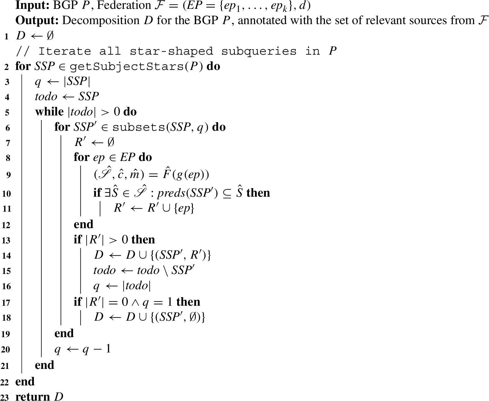
Cardinality estimation Given a query decomposition, the query planner estimates the cardinalities of all subexpressions in the decomposition. Given these estimations, the planner determines an efficient join order for the subexpressions. To this end, the subexpressions are ordered by increasing cardinality to minimize the number of intermediate results to be transferred during query execution. For a given subexpression
(1)
(2)
For the first case, we apply the StarJoinCardinality algorithm proposed by Neumann and Moerkotte [27] to estimate the cardinality for each source
We then sum up the estimations to aggregate the cardinalities across all sources:
In the second case (
Type I:
If both subject and predicate are bound in the triple pattern, we estimate the cardinality as the mean multiplicity values for all predicates and characteristic sets in all sources of the federation
Type II:
If just the subject is bound, we estimate the cardinality as the mean of the mean out-degrees
Type III:
If just the predicate is bound, we assume that the predicate occurs less frequently than the least frequent predicate in all estimated CSPF. The rationale for this is, if predicate p would occur more frequently, it would be very likely to be sampled. Thus, it can be assumed to be less frequent than any predicate that was sampled.
Type IV: (?s, ?p, ?o)
The estimated cardinality, is the sum of the sizes of the graphs in the federation:
For all remaining types of triple patterns, we estimate the cardinality to be 1.
Join ordering and query plan generation After estimating the cardinalities of all subexpressions in the decomposition, the query planner iteratively builds a left-deep plan by joining subexpressions ordered by increasing cardinality. In this query plan, each tuple
Limitations Note that the proposed query planner does not guarantee to obtain query plans that produce complete answers. This is due to two main reasons. First, the planner may fail to identify a source as relevant in the case that the relevant characteristic set is missing in the CSPF estimation. While the planner assumes all sources to be relevant in the case that none of the estimations include a matching predicate, it might be the case that the a CSPF estimation for one source is missing the relevant information and for another sources it does not.
Second, the greedy nature of our query decomposition approach presented in Algorithm 1 may produce query decompositions that yield incomplete results. For example, the decomposer may find a star-shaped subquery
Table 3
Characterization of the FedBench RDF graphs studied in the experiments
| General Properties | Characteristic Sets | ||||||||||
| RDF Graph | # Triples | # Subj. | # Pred. | # Obj. | |||||||
| Cross Domain | DBpedia | 42855253 | 9495865 | 1063 | 13636604 | 4.51 | 6.44 | 160062 | 1.69% | 66.31% | 95.23% |
| GeoNames | 107950085 | 7479714 | 26 | 35799392 | 14.43 | 2.81 | 673 | 0.01% | 19.76% | 99.07% | |
| Jamendo | 1049647 | 335925 | 26 | 440686 | 3.12 | 4.31 | 42 | 0.01% | 11.9% | 92.38% | |
| LinkedMDB | 6147996 | 694400 | 222 | 2052952 | 8.85 | 5.31 | 8459 | 1.22% | 62.64% | 97.65% | |
| NY Times | 335197 | 21666 | 36 | 191537 | 15.47 | 28.73 | 47 | 0.22% | 19.15% | 91.14% | |
| SW Dog Food | 103465 | 9948 | 118 | 35520 | 10.40 | 10.24 | 569 | 5.72% | 37.96% | 88.43% | |
| Life Science | ChEBI | 4772706 | 50477 | 28 | 772138 | 94.55 | 1853.09 | 978 | 1.94% | 39.57% | 96.71% |
| Drugbank | 517023 | 19693 | 119 | 276142 | 26.26 | 30.33 | 3419 | 17.36% | 79.7% | 81.3% | |
| KEGG | 1090830 | 34260 | 21 | 939258 | 31.84 | 165.88 | 67 | 0.2% | 11.94% | 92.83% | |
5.Evaluation
We empirically evaluate our contributions in two experimental studies. The first study focuses on analyzing the different components of our proposed approach to estimate the Characteristic Sets Profile Feature (CSFP) presented in Section 3. The second study aims to evaluate our CSPF estimations-based federated query planner which we presented in Section 4. We use the well-known federated querying benchmark FedBench [37] to investigate the effectiveness of our query planner and therefore, investigate the RDF graphs from FedBench in the first part of the evaluation as well. All raw experimental results are provided online under the DOI 10.5281/zenodo.4507242. The source code is provided on GitHub: (i) the sampling implementation,88 and (ii) the query planner.99
5.1.Characteristic sets profile feature estimation evaluation
We first empirically evaluate the different components of our approach to estimate the Characteristic Sets Profile Feature (CSPF). In the evaluation, we focus on the following core questions:
Q1 How do different sampling sizes influence the similarity measures?
Q2 What is the impact of different sampling methods on the similarity measures?
Q3 What are the effects of leveraging additional statistics in the projection functions?
Q4 How do different characteristics of the RDF graph influence the estimation?
We first present the setup of our experiments and analyze the results in Sections 5.1.1 and 5.1.2. Based on our findings, we answer the core questions in the final discussion in Section 5.1.3.
Fig. 2.
The cumulative relative coverage curve shows the ratio of triples covered with respect to the characteristic sets ordered by decreasing relative coverage.
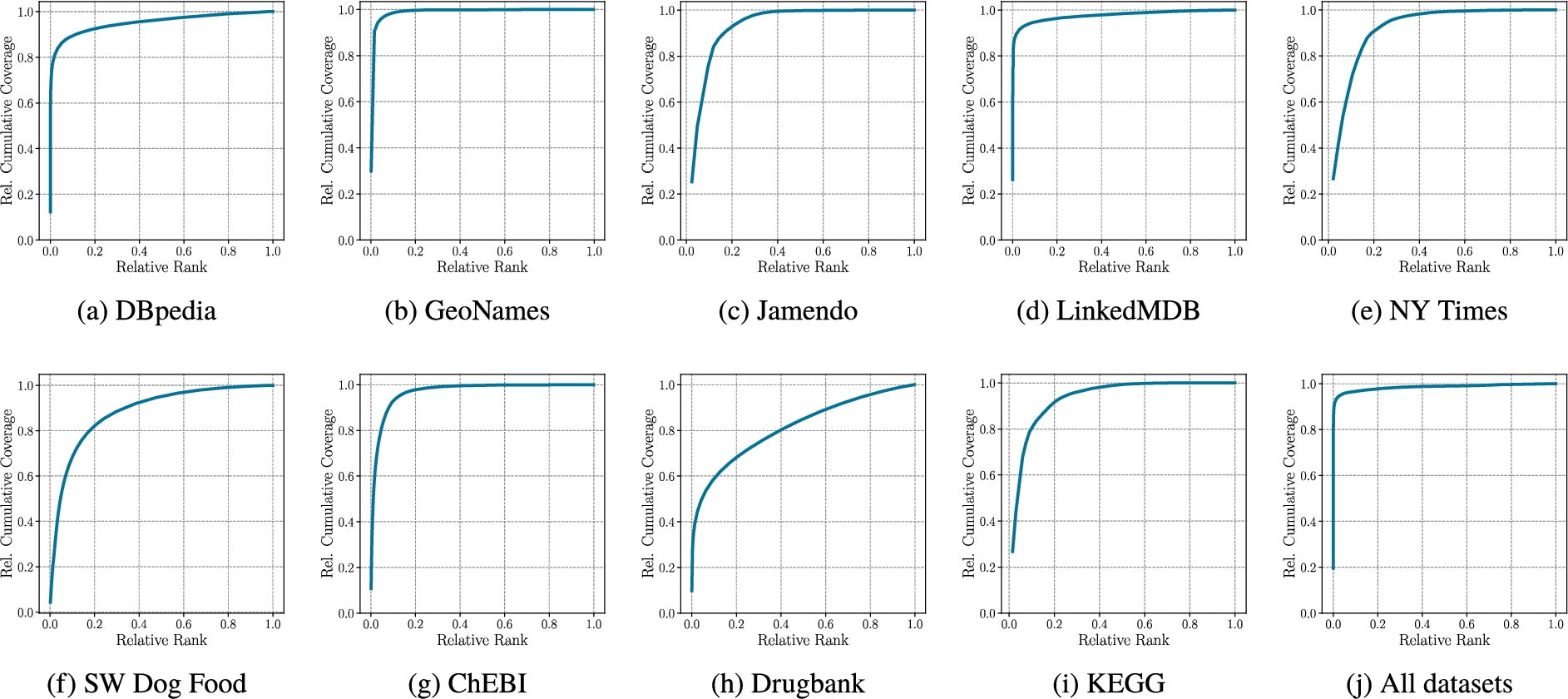
RDF graphs We select the six cross-domain and three Life Science RDF graphs from the FedBench benchmark [37] for our evaluation. An overview of the graphs’ properties is given in Table 3. The graphs differ in their general properties: the number of triples, the number of distinct subjects, predicates, and objects as well as the out-degree distribution. Moreover, the graphs differ with respect to their characteristic sets. The number of characteristic sets ranges from 42 to more than 160000. Theoretically, the number of potential characteristic sets in a graph is bound by the power set of its predicates. In practice, however, the number of distinct subjects in the graph is a stricter upper bound. Therefore, we provide the ratio of characteristic sets and distinct subjects (
Figure 2 shows the cumulative coverage curve of the characteristic sets for all graphs. The curve plots the cumulative coverage of the characteristics sets in a graph sorted by decreasing coverage (c.f. Equation (3)).
Sampling methods We study the presented unweighted, weighted, and hybrid sampling methods. We chose
Table 4
Mean similarity values
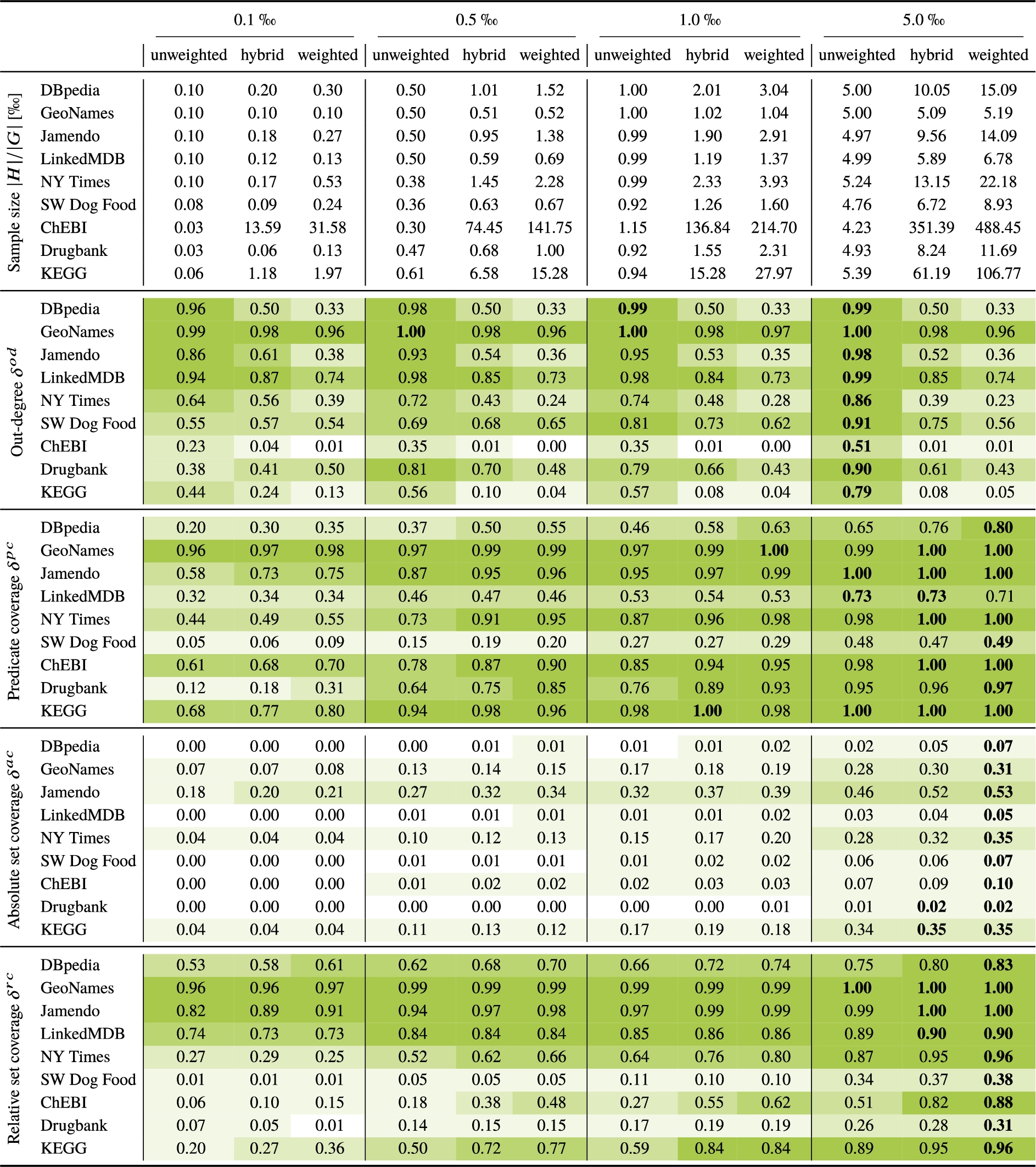
5.1.1.Structural similarity measures
Table 4 shows the structural similarity measures out-degree
Interestingly, there are also few cases where a higher sample size yields worse similarity results. For instance, the out-degree similarity
The two graphs KEGG and ChEBI have a high dispersion of the out-degree distribution with
Considering the absolute (
Comparing the different sampling methods (Q2), we observe that the unweighted sampling method outperforms the other methods for the out-degree similarity
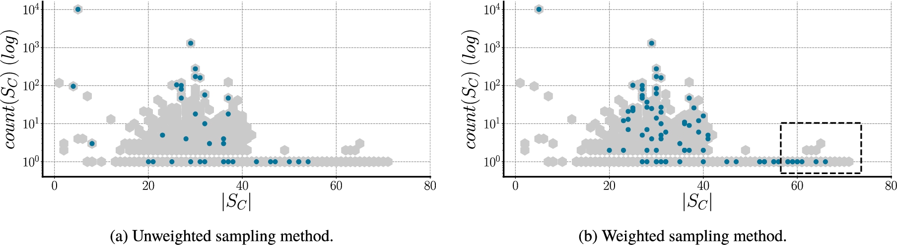
Fig. 3.
Sampled characteristic sets for Drugbank for one sample with a
Except for LinkedMDB, the unweighted sampling method exhibits the lowest predicate coverage similarity (
Fig. 4.
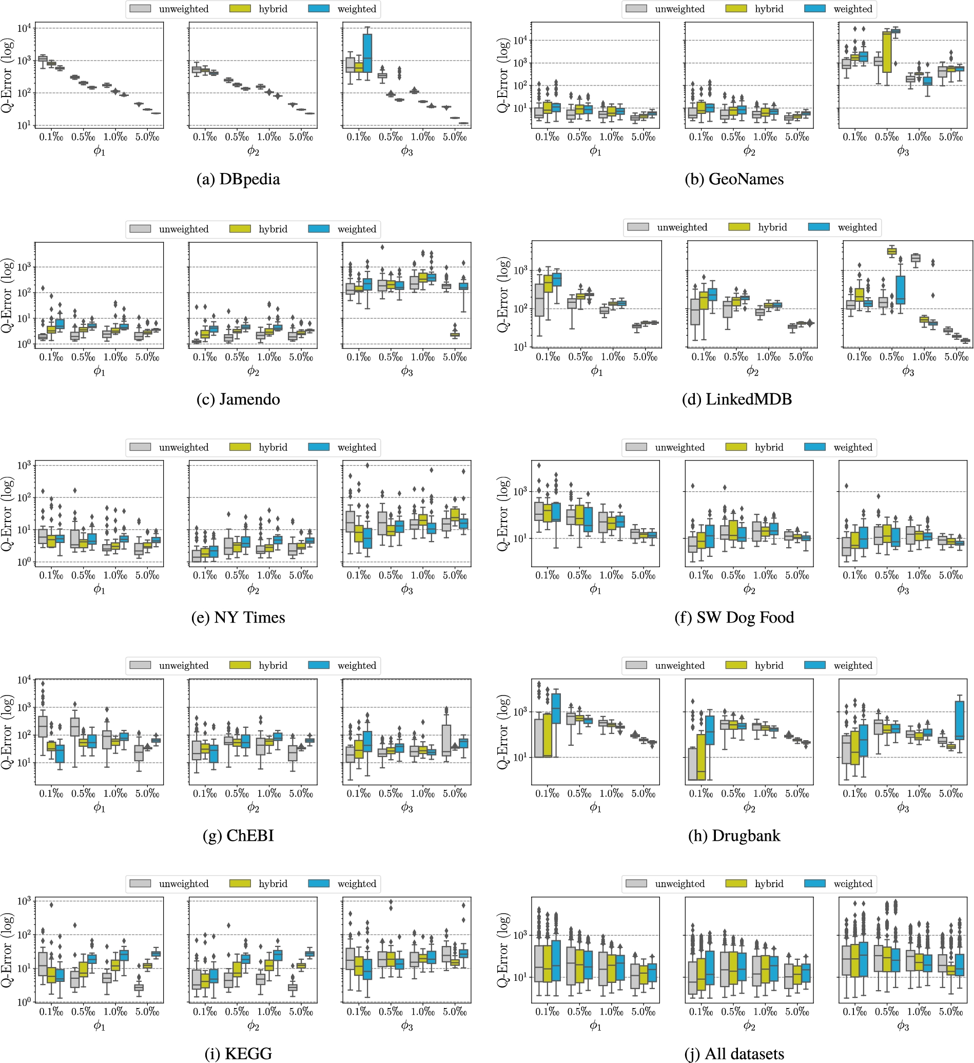
Box plots of the count estimation q-errors (lower is better) for each dataset, projection function, sample size and sampling method.
5.1.2.Statistical similarity measures
We now focus on the statistical similarity measures that assess the accuracy of the count and multiplicity estimations. In this evaluation, we concentrate on the q-errors due to their more natural interpretation, rather than the proposed similarity measures
Fig. 5.
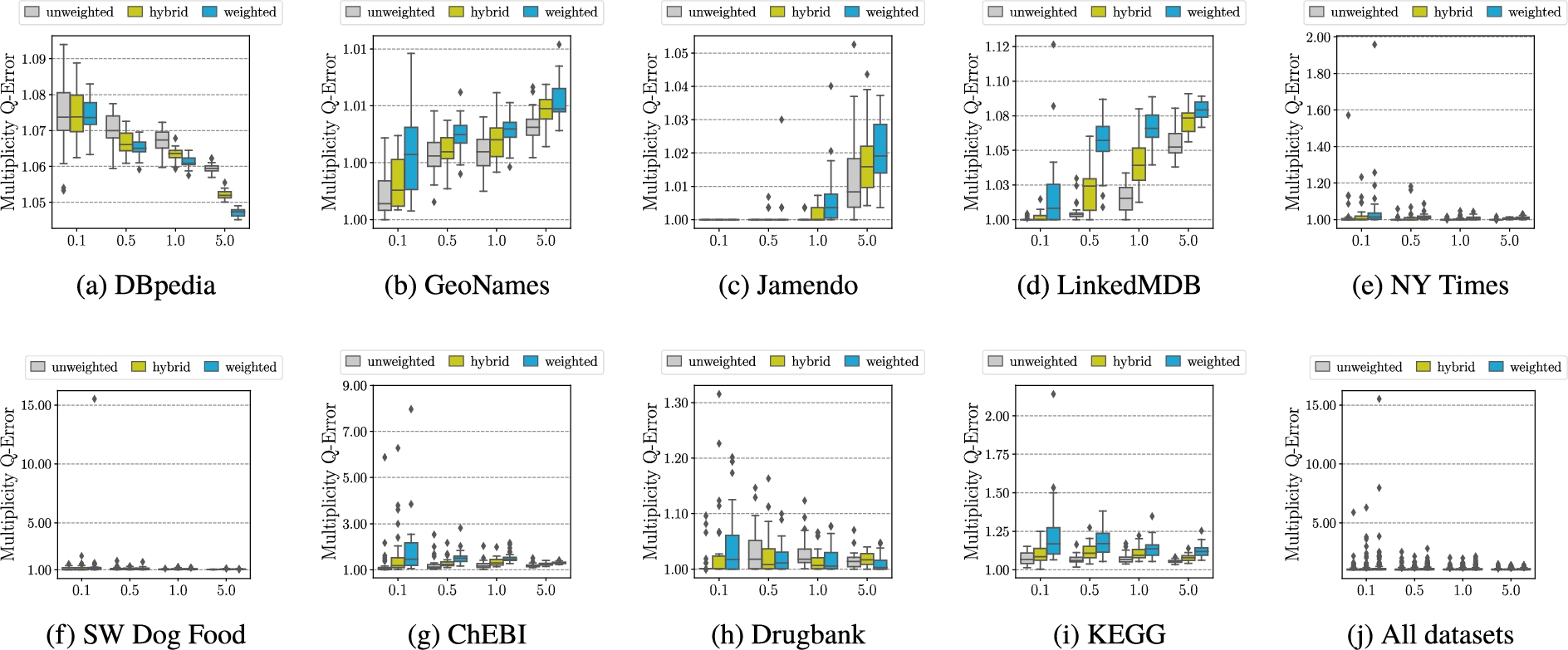
Box plots of the q-errors (lower is better) of the predicate multiplicity estimations for each dataset, sample size and sampling method.
Similar to the structural similarity measures, the results indicate an improvement in the estimations with larger sample sizes (Q1) in the majority of cases. Regarding the projection functions, this observation holds for the basic projection function
Comparing the different sampling methods (Q2), we observe a tendency of the smaller q-errors for the unweighted sampling method, especially for the basic projection function
Considering the characteristic set diversity of the graphs
Summarizing the results across all datasets for the count q-errors (cf. Fig. 4j), we observe that an increase in sample size (Q1) reduces the q-errors while simultaneously generating estimations for more characteristic sets. The unweighted sampling method (Q2) yields the lowest q-errors in the majority of cases and
Next, we focus on the estimations of the predicate multiplicities within the characteristic sets. Analogous to the count statistic, we concentrate on the q-errors in the evaluation and aggregate the values per sample by computing the mean over all its characteristic sets:
The box plots of the samples’ mean q-errors are shown in Fig. 5 for all graphs, sample sizes, and sampling methods. The first obvious observation is the substantially lower q-errors in comparison to the count statistic. This is because the range of the value to be estimated is lower. Typically, the same predicate is only used a few times for the same subject, with some exceptions that occur multiple times, such as rdf:type or rdfs:label. This is also reflected in the absolute differences, where the multiplicity q-errors are less affected by the sampling method and sample size. This indicates a uniform predicate usage within the characteristic sets with few outliers. In line with the results for the count statistic, in the majority of cases, an increasing sample size (Q1) improves the results. The results for the different sampling methods show better results for the unweighted sampling method for the majority (seven) of the graphs. The weighted sampling method shows slightly better results for DBpedia and Drugbank. Comparable to the results for the count statistics, the hybrid sampling method finds a balance between the other two sampling methods. Furthermore, the results indicate that multiplicities are more challenging to estimate for graphs with a high out-degree dispersion (Q4), such as ChEBI and KEGG. The best overall estimations are observed for GeoNames, which also has the lowest out-degree dispersion (
Concluding, as the summarized results in Fig. 5j show, the multiplicity statistic are estimated more accurately than count statistic with improving estimations for larger sample sizes (Q1), marginal differences comparing the sampling methods (Q2), and less diverse results for the different graph (Q4).
5.1.3.Final discussion
After providing a detailed presentation of our experimental results, we conclude the evaluation by providing answers to our core questions.
Q1: The results indicate that larger sample sizes have two major positive effects on the estimations. First, they improve both structural and statistical similarities measures of the estimations. Secondly, they allow for capturing and estimating the statistics for more characteristic sets and, therefore, potentially provide better support to applications that rely on these estimations.
Q2: Regarding the different sampling methods, we observe differences in the estimated profile features. On the one hand, the weighted sampling method tends to obtain larger samples for the same number of sampled subjects and, hence, yields slightly better structural similarity values. On the other hand, the unweighted sampling method obtains smaller samples and still obtains competitive structural similarity measures. Irrespective of the projection function, the unweighted sampling method outperforms the weighted sampling method w.r.t. the statistical similarity measures.
Q3: The analysis of the results showed that the first statistic-enhance projections function provides the best estimations. However, it only sightly outperforms the basic projection function with the differences diminishing with increasing sample size. The second statistics-enhanced projection function is outperformed by the others. Especially for graphs with a small diversity in characteristic sets, it yields higher estimation errors.
Q4: The investigation of the results showed that the structure of the RDF graph affects the similarity values. Especially the counts of the characteristic sets are misestimated for datasets with a large portion of exclusive characteristic sets and a larger diversity of characteristic sets. In such scenarios, larger sample sizes can help to improve the estimations.
Concluding all findings, a variety of factors, ranging from the sampling method to the structure of the RDF graphs, impact the quality of the characteristic sets profile feature estimation. Therefore, in our second evaluation, we investigate how the CSPF estimation can be leveraged in a specific application and how the estimations impact the performance of the application.
5.2.Federated query planner evaluation
After investigating the effectiveness of our approach to estimate profile features according to the similarity measures, we now focus on a particular application of the estimated features. We, therefore, study the performance of the proposed federated query planning approach that relies on CSPF estimations. In particular, we want to study the following core questions.
Q5 How do the CSPF estimations obtained from the unweighted and weighted sampling methods impact the effectiveness of federated query planning?
Q6 How do the CSPF estimations from different sample sizes impact the effectiveness of the plans?
Q7 What is the effect of the different projection functions on the query plan effectiveness?
Q8 How well do the structural similarity measures reflect the performance of the query plans?
We begin by introducing our experimental setup. We then provide a detailed evaluation and discussion of our experimental results in Section 5.2.1, which we conclude by answering our core questions in Section 5.2.2.
Benchmark and sampled statistics We study the effectiveness of the proposed query planning approach using the FedBench benchmark [37]. The benchmark consist of the 9 interlinked RDF graphs that are listed in Table 3, and which were also investigated in the previous evaluation. We selected 25 queries from the Cross Domain (CD1-CD7), Life Science (LS1-LS7), and Linked Data (LD1-LD11) queries. We used a subset of the estimated CSPF generated from the samples of the previous evaluation. In particular, we only considered the weighted and unweighted sampling methods, leading to a total of 2160 estimated CSPF.1111
As a baseline, we additionally computed the complete CSPF for all RDF graphs. In accordance with previous approaches [26,27], we reduce the number of characteristics sets in the profile feature to a maximum of 10000 characteristic sets per RDF graph.
Implementation We implemented the proposed federated query planning approach based on CROP [18] and nLDE [3]. We extended the query engine with an access operator for SPARQL endpoints and implemented our source selection, query decomposition, and left-linear query plan optimizer to create query execution plans. The RDF graphs in the federation are deployed with a single SPARQL endpoint per graph using Virtuoso v7.2..1212 We deployed all endpoints on a single machine (Debian Jessie 64 bit; CPU: 2x Intel(R) Xeon(R) CPU E5-2670 2.60GHz (16 physical cores); 256GB RAM) and execute the query engine on the same machine as well to avoid network latency.
We study the performance on each of the 30 samples for the 2 sampling methods (weighted and unweighted), 4 sample sizes (
Evaluation metrics We study the following metrics:
1. Execution Time: Elapsed time spent by the engine to complete the evaluation of a query in seconds. This includes time spent on query planning.
2. Number of requests: Number of requests performed by the engine to the SPARQL endpoints during the query execution.
3. Answer completeness: Percentage of total answers produced. We computed the complete answers by executing the queries over the union of all graphs.
4. Number of subexpressions: Number of subexpressions in the query decomposition to assess how well the predicate co-occurrence of the graphs is captured in the estimated CSPF.
5.2.1.Experimental results
An overview of the experimental results is provided in Table 5. The table shows the mean and median execution times, the mean number of requests, the mean percentage of answers produced, and the mean percentage of query executions reaching the timeout. We start with the results for the unweighted sampling method (Q5). Regarding the mean execution time, we observe the best performance for the unweighted sampling method with the largest sample size 5.0‰and the projection function
Table 5
Overview for the FedBench Queries. Mean and median execution times, mean number of requests, mean percentage of answers produces, and mean percentage of queries reaching the timeout. Best values per table are indicated in bold
| Unweighted | Baseline | ||||||||||||
| 0.1‰ | 0.5‰ | 1.0‰ | 5.0‰ | 1000‰ | |||||||||
| – | |||||||||||||
| Mean execution time [s] | 7.09 | 6.69 | 6.77 | 4.75 | 4.69 | 4.65 | 3.33 | 3.34 | 3.33 | 1.53 | 1.54 | 1.54 | 8.43 |
| Median execution time [s] | 0.66 | 0.63 | 0.64 | 0.42 | 0.44 | 0.44 | 0.42 | 0.43 | 0.46 | 0.62 | 0.61 | 0.63 | 1.01 |
| Mean number of requests | 241.95 | 229.97 | 229.76 | 159.46 | 159.06 | 155.02 | 113.94 | 113.95 | 111.2 | 45.69 | 45.69 | 45.7 | 173.92 |
| Answers [%] | 72.13 | 72.09 | 72.13 | 90.13 | 90.13 | 90.09 | 96.53 | 96.53 | 96.53 | 100.0 | 100.0 | 100.0 | 100.0 |
| Timeouts [%] | 3.6 | 3.6 | 3.6 | 1.47 | 1.47 | 1.47 | 0.93 | 0.93 | 0.93 | 0.0 | 0.0 | 0.0 | 4.0 |
| Weighted | Baseline | ||||||||||||
| 0.1‰ | 0.5‰ | 1.0‰ | 5.0‰ | 1000‰ | |||||||||
| – | |||||||||||||
| Mean execution time [s] | 9.24 | 7.61 | 8.46 | 2.84 | 1.89 | 1.98 | 4.45 | 4.13 | 4.49 | 6.08 | 6.11 | 6.45 | 8.43 |
| Median execution time [s] | 0.56 | 0.55 | 0.56 | 0.43 | 0.45 | 0.56 | 0.57 | 0.58 | 0.68 | 0.76 | 0.77 | 0.77 | 1.01 |
| Mean number of requests | 170.94 | 171.75 | 174.21 | 64.08 | 64.14 | 64.16 | 178.27 | 178.18 | 192.06 | 256.97 | 257.02 | 257.32 | 173.92 |
| Answers [%] | 81.33 | 81.73 | 81.69 | 97.2 | 98.0 | 98.0 | 96.8 | 97.07 | 96.8 | 96.0 | 96.0 | 96.0 | 100.0 |
| Timeouts [%] | 5.73 | 4.36 | 5.07 | 1.07 | 0.27 | 0.27 | 2.8 | 2.53 | 2.8 | 4.13 | 4.13 | 4.13 | 4.0 |
In contrast, the performance results differ for the weighted sampling method (Q5). The weighted sampling method with the second smallest sample size (0.5‰) yields the best performance. When comparing the results for the projection functions (Q7), we find similar results as for the unweighted sampling method, with only slight differences for the different projection functions. The results for the sample size (0.5‰) show the lowest average execution times and number of requests. Moreover, the query execution plans obtained for this sample size yields the highest answer completeness with
Hence, we focus on the results for the weighted sampling method in more detail to investigate the following observations: (i) a larger sample size in the weighted sampling does not entail better query execution performance, and (ii) the query planner with complete statistics is outperformed by the majority of configurations with estimated statistics. The mean execution times and mean number of requests (both log scale) per query and sample size for the weighted sampling method (all projection functions) are shown in Fig. 6. The trend of an increase in execution time with larger samples sizes is observable especially for the queries CD4 and LS3. For the majority of the remaining queries, we see a similar or even better performance with larger sample sizes according to execution times and number of requests. The observation that few outliers (especially CD4 and LS3) skew the overall average performance results is also true for the performance of the planner with the complete statistics.1313 Taking a closer look at the results for LS3, we find that for the sample size 0.5‰, the engine times out 3 times. Intriguingly, for the largest sample size (5.0‰) and also for the complete statistics, it reaches the timeout for all 90 executions. Similarly, for query CD4, larger sample sizes also lead to several executions reaching the timeout. The reason for these results lies in the cardinality estimation approach. We observe that CD4 and LS3 have a selective triple pattern in which the object is bound. The StarJoinCardinality algorithm tends to overestimate the cardinalities for stars with such triple patterns and the tendency of overestimating is higher with more characteristics sets that are taken into consideration.1414 As a result, this overestimation in the query CD4 and LS3 leads to a sub-optimal join ordering. For example, Fig. 7 shows the join ordering for CD4 obtained with one weighted sample with size 0.5‰and 5.0‰. The estimated cardinalities (in blue) and true cardinalities (in parenthesis) in this example reveal that due to the overestimation of the subexpression with the bound object (“Tarzan”), the planner chooses a sub-optimal join order in the case of the larger sample.
Fig. 6.
Mean performances for all FedBench queries for the weighted sampling method and averaged across all projection functions.
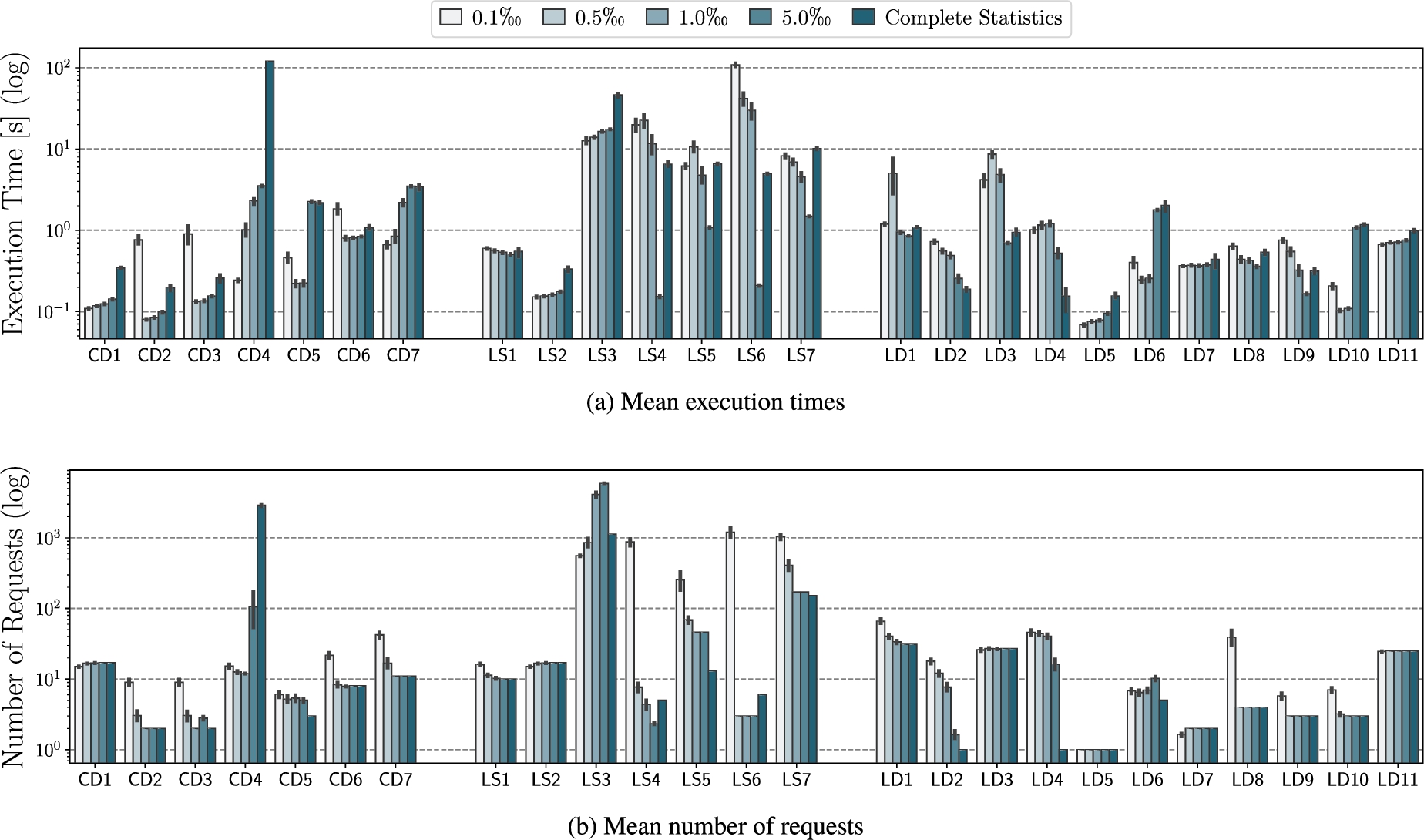
Fig. 7.
CD4: Join Ordering obtained by the query planner based on the estimated CSPF from one of the weighted samples. Indicate below is the estimated cardinality (blue) and the actual cardinality(in brackets).
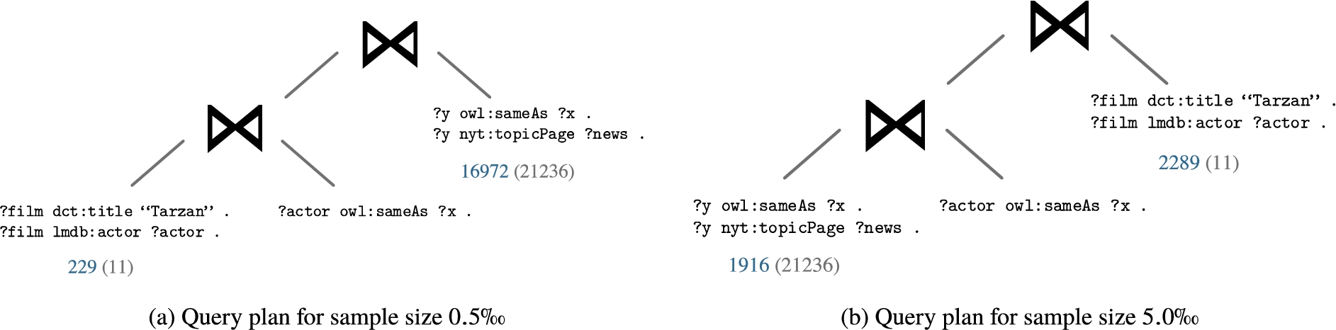
Fig. 8.
Relation between the answer completeness and the number of subexpression of the query plans and the structural similarity measures for the estimated CSPF. Sample size are indicated in color.
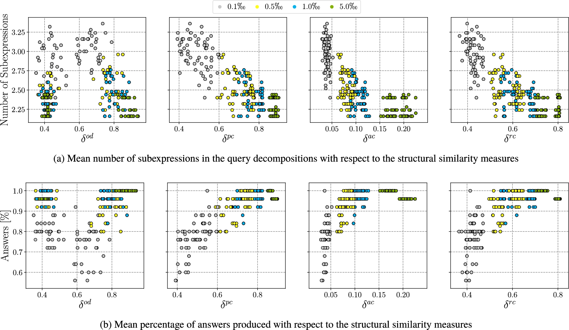
Finally, we want to examine whether the proposed structural similarity measures (c.f. Section 3.6) reflect the performance of the query plans obtained by our planning approach (Q8). To this end, we compare the impact of the out-degree similarity (
Similar to this observation, the results in Fig. 8b show that, there is no correlation between the answer completeness and the out-degree similarity
5.2.2.Final discussion
Concluding the evaluation of the experimental results for our query planning approach, we summarize the findings by providing answers to our core question.
Q5: The results show that the CSPF estimations obtained from the unweighted sampling method allow for determining the most efficient query plans. The difference in performance between the sampling methods is not due to the representativeness of the samples but rather due to sub-optimal join orderings caused by misestimated cardinalities for the weighted samples. This sub-optimal join led to time outs, which negatively affect the aggregated execution time and answer completeness of the weighted sampling. The lowest execution times and number of requests are observed for the unweighted sampling method with the largest sample size. For this configuration, all answers are produced and none of the query executions reach the timeout.
Q6: Regarding the results for different sample sizes, CSPF estimations obtained from larger samples using the unweighted sampling method improve the query execution performance. In contrast, the second smallest sample size yields the best results for the weighted sampling methods. In the latter case, the aggregated results are skewed due to few queries for which the approach overestimates the cardinality of subexpressions with a bound object. Adapting the cardinality estimation approach to better cope with sampled statistics could alleviate these shortcomings. The goal of the experiments is understanding how the increasing the sample sizes impacts the query execution performance. Note that determining exact samples sizes where the planner will yield the same plans as with full statistics is not feasible as it depends on the graphs and the queries.
Q7: The count estimations of the projection functions are used to estimate the cardinalities of the subexpressions in the decompositions. The results show that there is only a small difference in query execution performance for the different projection functions (ceteris paribus). We observed that, even if the projection functions achieve different accuracy, this barely affects the join ordering. This is because the relative differences between count estimations of the functions are consistent with the relative differences among the true counts.
Q8: Considering the structural similarity measures, the results suggest that the similarity measures predicate coverage and (absolute and relative) set coverage correlate with the number of subexpressions in the decomposition and answer completeness of the query plans. The correlation indicates that more efficient query plans can be obtained for CSPF estimation that representative according to these measures. This also underpins the effectiveness of the measures.
Summarizing the evaluation, we demonstrated the successful application of characteristics sets profile feature estimations to federated query planning. Overall, the unweighted sampling method with the largest sample size showed the best average performance. The experiments show that the proposed query planner provides a foundation to further develop query planning approaches that leverage estimated profile features obtained from RDF graph samples. For instance, future research could investigate source selection techniques as proposed in [35], but relying on samples to get the authority of subjects and objects in the graphs.
Limitations Finally, we want to discuss the limitations of the proposed query planner and experiments. The first limitation is the heuristic nature of the planner. As a result, there are no theoretical guarantees for the answer completeness of the query decomposition. For example, in case the planner finds at least one relevant source for a triple pattern in the estimated statistics, it assumes there are no additional relevant sources, which are not captured in the statistics. In other words, the query planner does not know what it does not know about. This limitation could potentially be overcome by obtaining additional information from the RDF graph, such as its distinct predicates, in the case that the expressivity of the query interface supports this. Secondly, our evaluation focuses on an implementation that combines query planning and execution based on CROP. Therefore, our insights are currently limited to this setup and future work should investigate our planner with other query execution engines (e.g. using SPARQL 1.1 queries). This would also allow for a direct comparison to Odyssey. Finally, additional federated benchmarks could be investigated to gain further insights.
Regardless, our experimental results still provide valuable insights into the potential of using sample-based statistics and summaries to support federated querying approaches without requiring access to the entire datasets of the federation members.
6.Related work
We now discuss related work on statistical profiling (Section 6.1), graph sampling (Section 6.2) and federated query processing (Section 6.3).
6.1.Statistical profiling
In the realm of statistical feature profiling for RDF graphs, a variety features and tools to assess them have been proposed. Zloch et al. [44] investigate statistical features of RDF graphs with the focus on the topological graph structure including degree-based, edge-based, centrality, and descriptive statistical measures. Consequently, these measures are not specific to RDF graphs and, in contrast to our work, do not capture the semantics on the instance or schema level of the data. Complementary, Fernández et al. [14] focus on RDF-specific measures. They propose various schema- and instance-level metrics to characterize RDF datasets that incorporate the particularities of RDF graphs. The metrics and the resulting statistics are tailored to the development of better RDF data storage solutions including data structures, indexes, and compression techniques by considering RDF data characteristics.
LODStats [6] is a statement-stream-based approach for gathering comprehensive statistics of RDF datasets. They present 32 instance- and schema-level statistical criteria covering both RDF-specific metrics as well as topological graph metrics. The authors aim to improve reuse, linking, revising, or querying Linked Open Data sources but do not discuss specific applications.
ProLOD
Finally, ExpLOD [20] is a tool for generating summaries of RDF datasets combining text labels and bisimulation contractions. These summaries include schema-level statistical information such as the class, predicate, and interlinking usage in the dataset. Similar to ProLOD
In this work, we propose a novel schema-level statistical profile feature based on characteristic sets that captures both the topological structure of the graph as well as its semantics. This statistical feature has not yet been addressed in related work. We demonstrate an application of estimations of this feature in federated query planning.
6.2.Graph sampling
Next, we focus on sampling approaches for graphs. We start by introducing related work on sampling large graphs and networks. Thereafter, we analyze RDF-specific sampling approaches and their applications.
Graph sampling A variety of approaches for sampling large non-RDF graphs have been proposed. Leskovec et al. [21] provide an overview of approaches suitable for obtaining representative samples from large graphs for scale-down sampling for static graphs and back-in-time sampling for evolving graphs. They consider the distributions of different structural properties of the graphs, denoted static graph patterns, as the criteria for evaluating the representativeness of the samples for scale-down sampling. These static graph patterns include, among others, the in-degree, out-degree, and cluster coefficient distributions. As a similarity measure to assess the representativeness of samples, they use the Kolmogorov-Smirnov D-statistic of the graph patterns’ distribution. They present three major categories of sampling approaches: (i) random node selection, (ii) random edge selection, and (iii) graph exploration. The results of their evaluation reveal that there is no single best solution and the authors conclude that an appropriate sampling algorithm and sample size depends on the specific application.
Ahmed et al. [5] present a detailed framework for the problem of graph sampling that focuses on large scale graphs. They identify two models of computation that are relevant when sampling from large graphs. The static model of computation allows for randomly accessing any location in the graph. The streaming model of computation merely allows for accessing edges in a sequential stream of edges. In their evaluation, the authors show that the proposed methods preserve key graph statistics of the graph (e.g., degree distributions, cluster coefficient distribution). Moreover, they demonstrate low space- and runtime-complexity that is in the order of edges in the sample for these methods.
Our sampling methods are a special case scale-down sampling of random node selection approaches according to [21], that only sample specific nodes, the entities of an RDF graph. However, in contrast to traditional graph sampling, we aim to generate representative samples for our specific statistical graph feature. Hence, the representativeness of a sample is given by the accuracy of the profile feature estimation.
RDF graph sampling Sampling approaches for RDF graphs have been proposed and applied to different problems as well. In the following, we will analyze example applications and show how sampling approaches are chosen according to those applications.
Debattista et al. [11] propose approximating specific quality metrics for large, evolving datasets based on samples. They argue that the exact computation of some quality metrics is too time-consuming and that an approximation is usually sufficient. In particular, they apply a sampling-based approach for the quality metrics (i) dereferenceability of URIs, and (ii) links to external data providers. They use the reservoir sampling approach [42] which randomly selects n items from a set of N elements with the equal probability
In their work, Rietveld et al. [34] aim to obtain samples that entail as many of the original answers to typical SPARQL queries. They use query logs from SPARQL endpoints to determine such typical queries. The sampling pipeline proposed by the authors consists of four steps and aims to obtain the parts of the graph that are relevant for answering the queries. First, they rewrite the original RDF graph as a directed unlabeled graph. On the resulting graph, they then compute the structural graph metrics PageRank, in-degree, and out-degree for all nodes. Thereafter, they use the structural graph metrics to rank the triples in the graph and generate the sample by selecting the top-k percent of all triples. The authors aim to obtain samples with a “more manageable size” [34] that produce answers to common SPARQL queries and hence, the samples’ representativeness is measured by the recall for those queries. As a result, the resulting samples may be biased towards more prominent entities in the graphs and less suitable to capture long-tail entities [8]. Different from our work, the goal is obtaining relevant samples which allow answering common queries. Therefore, these samples are not representative in our sense with regards to the semantic and statistical features.
Soulet et al. [39] focus on analytical queries, which are typically too expensive to be executed directly over public SPARQL endpoints. They propose separating the computation of such expensive queries by executing them over random samples of the RDF graph. Due to the properties of the queries, the values for the aggregations converge as they are executed over increasingly larger portions of the graph. As a result, the authors do not rely on the necessity of each sample to be representative according to the aggregates, but rely on the convergence of the aggregates towards the true value with an increasing number of samples. Similar to Soulet et al. [39], our work is motivated by the restrictions that occur especially in decentralized scenarios with large, evolving datasets where it is not feasible to have local access to every dataset. Different from [39], we aim to sample the data in such a fashion that a single sample can be used to estimate the statistical profile feature and do not rely on the convergence properties induced by increasing sample sizes.
6.3.Profiling-based federated query processing
We demonstrate how the profile features estimations can be applied to federated query processing. Therefore, in this section, we analyze other types of pre-computed statistics leveraged by federated query engines to determine efficient plans.
ANAPSID [4] is an adaptive federated query engine that leverages a Catalog with high-level statistics on the members in the federation. This catalog contains a list of the predicates present in each data member in the federation and is used by the engine to perform the source selection and query decomposition.
More fine-grained statistics are leveraged by the following approaches. SPLENDID [15] uses indexes built from VoID descriptions for query planning. These indexes additionally hold information on the occurrences of predicates within the classes of the sources. In combination with ASK queries, the indexes are used to decompose the query into subqueries to be evaluated at the sources in the federation. HiBISCuS [35] is a source selection approach that employs data summaries to prune the relevant sources. The data summaries are comprised of the capabilities of a data source which consists of the subject and object authorities for all predicates in a data source. These summaries allow for deciding which source will contribute to the final query answers according to the authorities of the subjects and objects they contain. CostFed [36] is a cost model-based planner using an index with statistic profiles on the sources, so-called Data Summaries. They extend the data summaries from HiBISCus with additional information on both the distribution of objects and subjects per predicates. In addition to source selection and query decomposition, the additional statistics are used in their cost model to estimate the cost of alternative query plans. Similar to CostFed, SemaGrow [10] leverages a metadata to estimate the cost of alternative query plans. The statistics include the number of distinct subjects, predicates, and objects as well as the total number of triples that match a given triple pattern. These statistics are used to estimate the join cardinalities in their cost model. Finally, Odyssey [26] relies on the characteristic sets of the federation members. Additionally, the characteristics pairs and federated characteristic pairs are used to capture links between entities within and across the federation members.
Our approach also uses statistics to perform source selection, query decomposition, and join ordering to obtain efficient query plans. Specifically, our approach leverages characteristics sets similar to Odyssey [26]. In contrast to the aforementioned approaches, however, our approach does not require the complete statistics but is specifically designed to handle estimated statistics from RDF graph samples. As a result, our approach aims to leverage the estimated statistics as much as possible and is also able to cope with potentially misestimated or missing statistics.
7.Conclusion
In this work, we presented an approach to estimate RDF dataset profile features and an application of those estimations in federated SPARQL query planning. Specifically, we focused on the characteristic set profile features as it captures not only structural but also semantic properties of RDF graphs. We proposed a sampling-based approach that utilizes a projection function to estimate characteristic set profile feature statistics (). Furthermore, we introduced four structural and two statistical similarity measures that allow for assessing the representativeness of the generated feature estimations. In our experimental study, we investigated the effectiveness of the proposed estimation approach using these similarity measures (). The evaluation showed that our approach obtains representative feature estimations according to the structural similarity measure. In contrast, the lower statistical similarity values showed that the count distributions of characteristics sets in the RDF graphs are more challenging to estimate. These results highlight that the samples capture structural aspects while it is difficult to capture the distribution of the characteristic sets.
The second main contribution of this work focused on an application of the proposed feature estimations to better understand the practical implications of their representativeness (). We proposed a federated query planning approach that leverages the estimated characteristic set profile features to perform source selection, query decomposition, and join ordering. The query planner is based on insights from existing characteristic set-based query planning strategies. However, it is adapted such that it can handle limited and potentially inaccurate information in the profile feature estimations. The results of our experiments on the FedBench benchmark illustrated the feasibility of using estimated profile features. Overall, we found the best query plans are obtained for the feature estimations using the unweighted sampling method with improvements for larger sample sizes. Moreover, the results revealed that the capability of obtaining more efficient query plans with respect to the number of subexpressions and answer completeness is also reflected in the structural similarity measures ().
Future work will focus on two directions. The first direction is extending our profile feature estimation approach with further sampling approaches that make use of additional information, such as query logs, to better capture the relevant parts of the RDF graphs. Besides, our approach can be extended to estimate other profile features. The second area of research is the application of the feature estimations to other problems. It would be worth investigating how other applications can benefit from the estimated profile features. Furthermore, we aim to improve the query planning approach by (i) leveraging further information that can be obtained from the samples, and (ii) implementing a hybrid planning strategy that not only relies on the estimated statistics. Finally, an evaluation of our query planner in additional federations will support a better understanding of the advantages and limitations of our approach.
Notes
4 In the remainder of this work, we assume prefixes as given in https://prefix.cc.
7 Alternatively, the planner could use ASK queries to determine which source is relevant. However, as we want to investigate the effectiveness of the estimated statistics, the proposed planner only relies on the estimated CSPF.
10 The degree of a characteristic set is given by the average degree of the entities belonging to it. The degree is therefore a combination of its size (number of predicates) and the predicates’
11 The previous experimental results suggest that the hybrid sampling method balances the two opposing (weighted and unweighted) sampling methods. We therefore assume that the estimated CSPF based on the hybrid samples will exhibit a similar performance in the following experiments. As a result, we only focus on the edge cases, that is weighted and unweighted samples.
13 Note that the query planner is designed to handle estimated statistics. Therefore, a query planner that fully leverages the complete statistics, e.g., with the (federated) characteristic pairs, would potentially obtain a more efficient query plan.
14 This is due to the fact that the number of relevant characteristic sets for a triple pattern
Acknowledgements
This work was supported by the grant QUOCA (FKZ 01IS17042) from the German Federal Ministry of Education and Research (BMBF).
Appendices
Appendix
AppendixEfficiency of CSPF computation
Part of the motivation of this work is the fact that computing and estimating CSPF over samples of the original graph reduces the computational effort. As discussed in Section 3.5, the computation method needs to be tailored to the access methods of the RDF graph. To showcase the reduction in computational effort when computing CSPF from samples, we focus on a single, general case and we assume the RDF graphs to be given as edge lists (i.e., n-triples files).
Algorithm 2:
Characteristic set profile feature creation
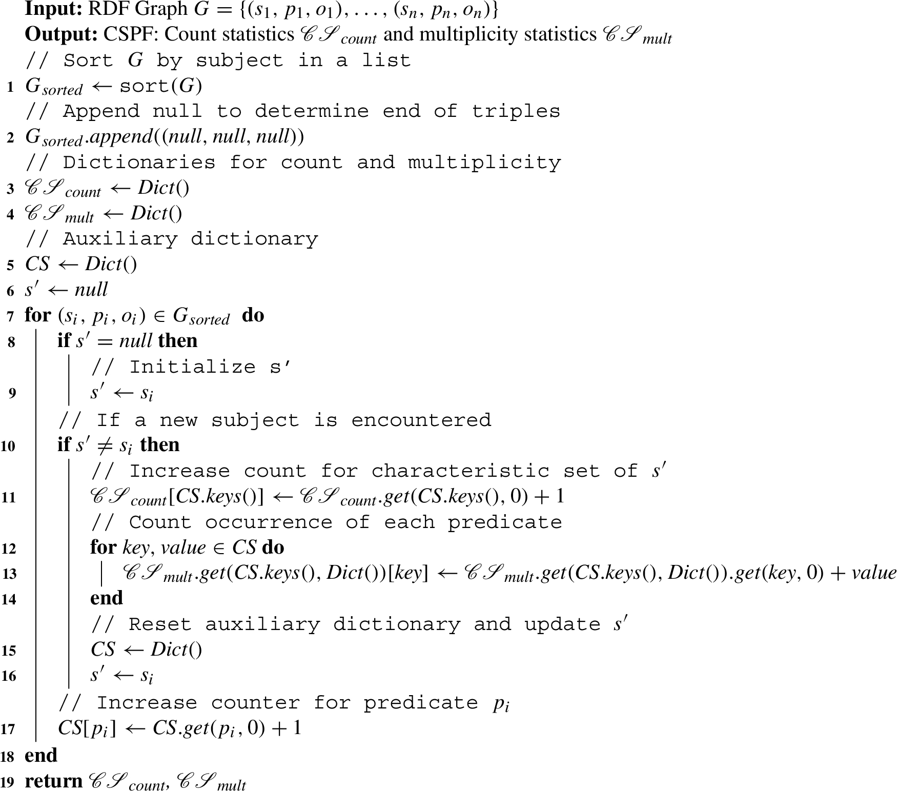
Algorithm The algorithm first sorts the triples in the graph G by subject. Thereafter, it iterates the sorted list of triples, determining the characteristic set per subject and storing the corresponding statistics in a hash table or dictionary. This process is detailed in Algorithm 2.
Central to the computation are dictionaries
Fig. 9.
Runtimes (log-scale) for computing the CSPF for the different sample sizes and the complete RDF graphs.
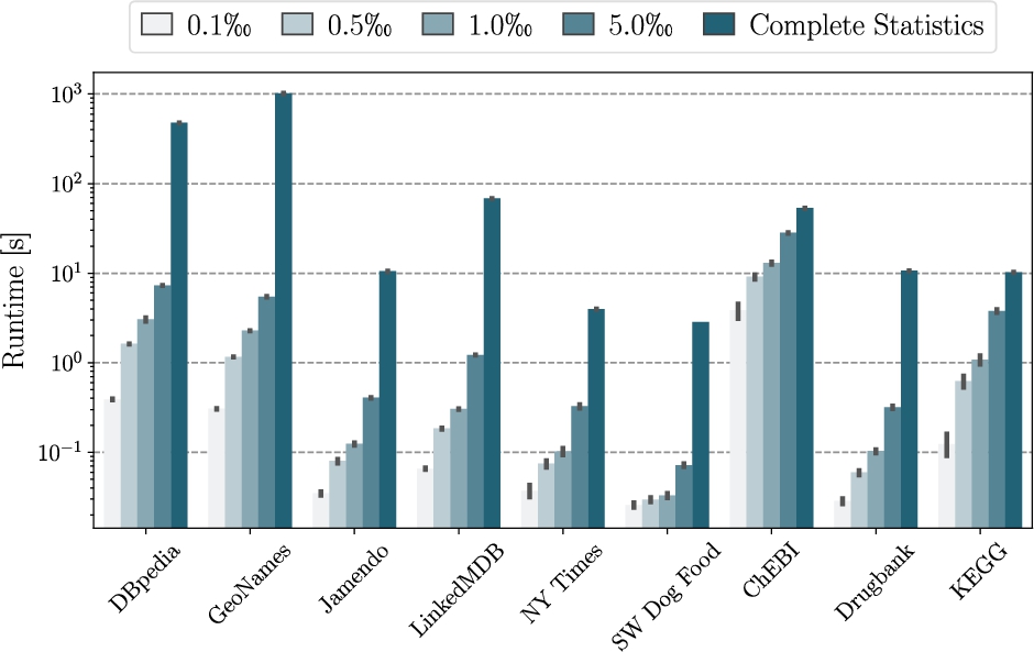
Efficiency results In Fig. 9, the mean runtimes for computing the CSPF are summarized per sample size and for the entire original graph. For the sake of comparability, the triples were randomly shuffled before computing the CSPF. For each of the 90 samples per dataset and sample size, the CSPF was computed once and the runtimes averaged across the 90 measurements. For the original graphs, this process was repeated 10 times to obtain an average runtime value. The results indicate a substantial reduction in the runtimes for computing the CSPF for the samples than the original graphs (note the log-scale for the runtimes). In addition, the gain in efficiency also depends on the structure of the RDF graph, such as its out-degree dispersion.
References
[1] | Z. Abedjan, T. Grütze, A. Jentzsch and F. Naumann, Profiling and mining RDF data with ProLOD++, in: Proceedings of ICDE, (2014) . doi:10.1109/ICDE.2014.6816740. |
[2] | M. Acosta, O. Hartig and J.F. Sequeda, Federated RDF query processing, in: Encyclopedia of Big Data Technologies, S. Sakr and A.Y. Zomaya, eds, Springer, (2019) . doi:10.1007/978-3-319-63962-8_228-1. |
[3] | M. Acosta and M. Vidal, Networks of linked data eddies: An adaptive web query processing engine for RDF data, in: The Semantic Web – ISWC 2015 – 14th International Semantic Web Conference, Proceedings, Part i, Bethlehem, PA, USA, October 11–15, 2015, M. Arenas, Ó. Corcho, E. Simperl, M. Strohmaier, M. d’Aquin, K. Srinivas, P. Groth, M. Dumontier, J. Heflin, K. Thirunarayan and S. Staab, eds, Lecture Notes in Computer Science, Vol. 9366: , Springer, (2015) , pp. 111–127. doi:10.1007/978-3-319-25007-6_7. |
[4] | M. Acosta, M. Vidal, T. Lampo, J. Castillo and E. Ruckhaus, ANAPSID: An adaptive query processing engine for SPARQL endpoints, in: The Semantic Web – ISWC 2011 – 10th International Semantic Web Conference, Proceedings, Part I, Bonn, Germany, October 23–27, 2011, (2011) , pp. 18–34. doi:10.1007/978-3-642-25073-6_2. |
[5] | N.K. Ahmed, J. Neville and R.R. Kompella, Network sampling: From static to streaming graphs, TKDD 8: (2) ((2013) ), 7:1–7:56. doi:10.1145/2601438. |
[6] | S. Auer, J. Demter, M. Martin and J. Lehmann, LODStats – an extensible framework for high-performance dataset analytics, in: Poceedings of EKAW, (2012) , pp. 353–362. doi:10.1007/978-3-642-33876-2_31. |
[7] | C. Böhm, F. Naumann, Z. Abedjan, D. Fenz, T. Grütze, D. Hefenbrock, M. Pohl and D. Sonnabend, Profiling linked open data with ProLOD, in: Workshops Proceedings of the 26th International Conference on Data Engineering, ICDE, (2010) , pp. 175–178. doi:10.1109/ICDEW.2010.5452762. |
[8] | E. Cao, D. Wang, J. Huang and W. Hu, Open knowledge enrichment for long-tail entities, in: WWW ’20: The Web Conference 2020, Taipei, Taiwan, April 20–24, 2020, (2020) , ACM/IW3C2 pp. 384–394. doi:10.1145/3366423.3380123. |
[9] | S. Cebiric, F. Goasdoué, H. Kondylakis, D. Kotzinos, I. Manolescu, G. Troullinou and M. Zneika, Summarizing semantic graphs: A survey, VLDB, J. 28: (3) ((2019) ), 295–327. doi:10.1007/s00778-018-0528-3. |
[10] | A. Charalambidis, A. Troumpoukis and S. Konstantopoulos, SemaGrow: Optimizing federated SPARQL queries, in: Proceedings of the 11th International Conference on Semantic Systems, SEMANTICS 2015, Vienna, Austria, September 15–17, 2015, sA. Polleres, T. Pellegrini, S. Hellmann and J.X. Parreira, eds, ACM, (2015) , pp. 121–128. doi:10.1145/2814864.2814886. |
[11] | J. Debattista, S. Londoño, C. Lange and S. Auer, Quality assessment of linked datasets using probabilistic approximation, in: Proceedings of ESWC, (2015) . doi:10.1007/978-3-319-18818-8_14. |
[12] | S. Dietze, E. Demidova and K. Todorov, RDF dataset profiling, in: Encyclopedia of Big Data Technologies, S. Sakr and A.Y. Zomaya, eds, Springer, (2019) . doi:10.1007/978-3-319-63962-8_288-1. |
[13] | M.B. Ellefi, Z. Bellahsene, J.G. Breslin, E. Demidova, S. Dietze, J. Szymanski and K. Todorov, RDF dataset profiling – a survey of features, methods, vocabularies and applications, Semantic Web 9: (5) ((2018) ), 677–705. doi:10.3233/SW-180294. |
[14] | J.D. Fernández, M.A. Martínez-Prieto, P. de la Fuente Redondo and C. Gutiérrez, Characterising RDF data sets, J. Inf. Sci. 44: (2) ((2018) ), 203–229. doi:10.1177/0165551516677945. |
[15] | O. Görlitz and S. Staab, SPLENDID: SPARQL endpoint federation exploiting VOID descriptions, in: Proceedings of the Second International Workshop on Consuming Linked Data (COLD2011), Bonn, Germany, October 23, 2011, O. Hartig, A. Harth and J.F. Sequeda, eds, CEUR Workshop Proceedings, Vol. 782: , (2011) , CEUR-WS.org, http://ceur-ws.org/Vol-782/GoerlitzAndStaab_COLD2011.pdf. |
[16] | A. Gubichev and T. Neumann, Exploiting the query structure for efficient join ordering in SPARQL queries, in: Proceedings of EDBT, (2014) . doi:10.5441/002/edbt.2014.40. |
[17] | L. Heling and M. Acosta, Estimating characteristic sets for RDF dataset profiles based on sampling, in: The Semantic Web – 17th International Conference, ESWC 2020, Proceedings, Heraklion, Crete, Greece, May 31–June 4, 2020, A. Harth, S. Kirrane, A.N. Ngomo, H. Paulheim, A. Rula, A.L. Gentile, P. Haase and M. Cochez, eds, Lecture Notes in Computer Science, Vol. 12123: , Springer, (2020) , pp. 157–175. doi:10.1007/978-3-030-49461-2_10. |
[18] | L. Heling and M. Acosta, Cost- and robustness-based query optimization for linked data fragments, in: ISWC (1), Lecture Notes in Computer Science, Vol. 12506: , Springer, (2020) , pp. 238–257. |
[19] | T. Johnson, Data profiling, in: Encyclopedia of Database Systems, L. Liu and M.T. Özsu, eds, 2nd edn, Springer, (2018) . doi:10.1007/978-1-4614-8265-9_601. |
[20] | S. Khatchadourian and M.P. Consens, ExpLOD: Summary-based exploration of interlinking and RDF usage in the linked open data cloud, in: Proceedings of ESWC, (2010) , pp. 272–287. doi:10.1007/978-3-642-13489-0_19. |
[21] | J. Leskovec and C. Faloutsos, Sampling from large graphs, in: Proceedings of ACM SIGKDD, (2006) , pp. 631–636. doi:10.1145/1150402.1150479. |
[22] | M.N. Mami, D. Graux, S. Scerri, H. Jabeen, S. Auer and J. Lehmann, Uniform access to multiform data lakes using semantic technologies, in: Proceedings of the 21st International Conference on Information Integration and Web-Based Applications & Services, iiWAS 2019, Munich, Germany, December 2–4, 2019, ACM, (2019) , pp. 313–322. doi:10.1145/3366030.3366054. |
[23] | M.V. Mannino, P. Chu and T. Sager, Statistical profile estimation in database systems, ACM Comput. Surv. 20: (3) ((1988) ), 191–221. doi:10.1145/62061.62063. |
[24] | M. Meimaris, G. Papastefanatos, N. Mamoulis and I. Anagnostopoulos, Extended characteristic sets: Graph indexing for SPARQL query optimization, in: Proceedings of ICDE, (2017) . doi:10.1109/ICDE.2017.106. |
[25] | G. Moerkotte, T. Neumann and G. Steidl, Preventing bad plans by bounding the impact of cardinality estimation errors, PVLDB 2: (1) ((2009) ), 982–993, http://www.vldb.org/pvldb/2/vldb09-657.pdf. doi:10.14778/1687627.1687738. |
[26] | G. Montoya, H. Skaf-Molli and K. Hose, The odyssey approach for optimizing federated SPARQL queries, in: Proceedings of ISWC, (2017) . doi:10.1007/978-3-319-68288-4_28. |
[27] | T. Neumann and G. Moerkotte, Characteristic sets: Accurate cardinality estimation for RDF queries with multiple joins, in: Proceedings of ICDE, (2011) . doi:10.1109/ICDE.2011.5767868. |
[28] | T. Neumann and G. Weikum, The RDF-3X engine for scalable management of RDF data, VLDB J. 19: (1) ((2010) ), 91–113. doi:10.1007/s00778-009-0165-y. |
[29] | M. Newman, Networks, Oxford University Press, (2018) . |
[30] | N.F. Noy, Y. Gao, A. Jain, A. Narayanan, A. Patterson and J. Taylor, Industry-scale knowledge graphs: Lessons and challenges, Commun. ACM 62: (8) ((2019) ), 36–43. doi:10.1145/3331166. |
[31] | J.Z. Pan, G. Vetere, J.M. Gómez-Pérez and H. Wu (eds), Exploiting Linked Data and Knowledge Graphs in Large Organisations, Springer, (2017) . ISBN 978-3-319-45652-2. doi:10.1007/978-3-319-45654-6. |
[32] | M. Pham, L. Passing, O. Erling and P.A. Boncz, Deriving an emergent relational schema from RDF data, in: Proceedings of the 24th International Conference on World Wide Web, WWW 2015, Florence, Italy, May 18–22, 2015, A. Gangemi, S. Leonardi and A. Panconesi, eds, ACM, (2015) , pp. 864–874. doi:10.1145/2736277.2741121. |
[33] | B.F. Ribeiro, P. Wang, F. Murai and D. Towsley, Sampling directed graphs with random walks, in: Proceedings of the IEEE INFOCOM 2012, (2012) , pp. 1692–1700. doi:10.1109/INFCOM.2012.6195540. |
[34] | L. Rietveld, R. Hoekstra, S. Schlobach and C. Guéret, Structural properties as proxy for semantic relevance in RDF graph sampling, in: Proceedings of ISWC, (2014) . doi:10.1007/978-3-319-11915-1_6. |
[35] | M. Saleem and A.N. Ngomo, HiBISCuS: Hypergraph-based source selection for SPARQL endpoint federation, in: Proceedings of ESWC, (2014) , pp. 176–191. doi:10.1007/978-3-319-07443-6_13. |
[36] | M. Saleem, A. Potocki, T. Soru, O. Hartig and A.N. Ngomo, CostFed: Cost-based query optimization for SPARQL endpoint federation, in: Proceedings of the 14th International Conference on Semantic Systems, SEMANTICS 2018, Vienna, Austria, September 10–13, 2018, (2018) , pp. 163–174. doi:10.1016/j.procs.2018.09.016. |
[37] | M. Schmidt, O. Görlitz, P. Haase, G. Ladwig, A. Schwarte and T. Tran, FedBench: A benchmark suite for federated semantic data query processing, in: The Semantic Web – ISWC 2011 – 10th International Semantic Web Conference, Proceedings, Part I, Bonn, Germany, October 23–27, 2011, L. Aroyo, C. Welty, H. Alani, J. Taylor, A. Bernstein, L. Kagal, N.F. Noy and E. Blomqvist, eds, Lecture Notes in Computer Science, Vol. 7031: , Springer, (2011) , pp. 585–600. doi:10.1007/978-3-642-25073-6_37. |
[38] | M. Schmidt, M. Meier and G. Lausen, Foundations of SPARQL query optimization, in: Database Theory – ICDT 2010, 13th International Conference, Proceedings, Lausanne, Switzerland, March 23–25, 2010, L. Segoufin, ed., ACM International Conference Proceeding Series, ACM, (2010) , pp. 4–33. doi:10.1145/1804669.1804675. |
[39] | A. Soulet and F.M. Suchanek, Anytime large-scale analytics of linked open data, in: Proceedings of ISWC, (2019) . doi:10.1007/978-3-030-30793-6_33. |
[40] | R. Verborgh, M.V. Sande, O. Hartig, J.V. Herwegen, L.D. Vocht, B.D. Meester, G. Haesendonck and P. Colpaert, Triple pattern fragments: A low-cost knowledge graph interface for the Web, J. Web Semant. 37–38: ((2016) ), 184–206. doi:10.1016/j.websem.2016.03.003. |
[41] | M. Vidal, E. Ruckhaus, T. Lampo, A. Martínez, J. Sierra and A. Polleres, Efficiently joining group patterns in SPARQL queries, in: The Semantic Web: Research and Applications, 7th Extended Semantic Web Conference, ESWC 2010, Proceedings, Part I, Heraklion, Crete, Greece, May 30–June 3, 2010, L. Aroyo, G. Antoniou, E. Hyvönen, A. ten Teije, H. Stuckenschmidt, L. Cabral and T. Tudorache, eds, Lecture Notes in Computer Science, Vol. 6088: , Springer, (2010) , pp. 228–242. doi:10.1007/978-3-642-13486-9_16. |
[42] | J.S. Vitter, Random sampling with a reservoir, ACM Trans. Math. Softw. 11: (1) ((1985) ), 37–57. doi:10.1145/3147.3165. |
[43] | A. Zaveri, A. Rula, A. Maurino, R. Pietrobon, J. Lehmann and S. Auer, Quality assessment for linked data: A survey, Semantic Web 7: (1) ((2016) ), 63–93. doi:10.3233/SW-150175. |
[44] | M. Zloch, M. Acosta, D. Hienert, S. Dietze and S. Conrad, A software framework and datasets for the analysis of graph measures on RDF graphs, in: The Semantic Web – 16th International Conference, ESWC 2019, Proceedings, Portorož, Slovenia, June 2–6, 2019, P. Hitzler, M. Fernández, K. Janowicz, A. Zaveri, A.J.G. Gray, V. López, A. Haller and K. Hammar, eds, Lecture Notes in Computer Science, Vol. 11503: , Springer, (2019) , pp. 523–539. doi:10.1007/978-3-030-21348-0_34. |


