
High-level ETL for semantic data warehouses
Abstract
The popularity of the Semantic Web (SW) encourages organizations to organize and publish semantic data using the RDF model. This growth poses new requirements to Business Intelligence technologies to enable On-Line Analytical Processing (OLAP)-like analysis over semantic data. The incorporation of semantic data into a Data Warehouse (DW) is not supported by the traditional Extract-Transform-Load (ETL) tools because they do not consider semantic issues in the integration process. In this paper, we propose a layer-based integration process and a set of high-level RDF-based ETL constructs required to define, map, extract, process, transform, integrate, update, and load (multidimensional) semantic data. Different to other ETL tools, we automate the ETL data flows by creating metadata at the schema level. Therefore, it relieves ETL developers from the burden of manual mapping at the ETL operation level. We create a prototype, named Semantic ETL Construct (SETLCONSTRUCT), based on the innovative ETL constructs proposed here. To evaluate SETLCONSTRUCT, we create a multidimensional semantic DW by integrating a Danish Business dataset and an EU Subsidy dataset using it and compare it with the previous programmable framework SETLPROG in terms of productivity, development time, and performance. The evaluation shows that 1) SETLCONSTRUCT uses 92% fewer Number of Typed Characters (NOTC) than SETLPROG, and SETLAUTO (the extension of SETLCONSTRUCT for generating ETL execution flows automatically) further reduces the Number of Used Concepts (NOUC) by another 25%; 2) using SETLCONSTRUCT, the development time is almost cut in half compared to SETLPROG, and is cut by another 27% using SETLAUTO; and 3) SETLCONSTRUCT is scalable and has similar performance compared to SETLPROG. We also evaluate our approach qualitatively by interviewing two ETL experts.
1.Introduction
Semantic Web (SW) technologies enable adding a semantic layer over the data; thus, the data can be processed and effectively retrieved by both humans and machines. The Linked Data (LD) principles are the set of standard rules to publish and connect data using semantic links [9]. With the growing popularity of the SW and LD, more and more organizations natively manage data using SW standards, such as Resource Description Framework (RDF), RDF-Schema (RDFs), the Web Ontology Language (OWL), etc. [17]. Moreover, one can easily convert data given in another format (database, XML, JSON, etc.) into RDF format using an RDF Wrappers [8]. As a result, a lot of semantic datasets are now available in different data portals, such as DataHub,11 Linked Open Data Cloud22 (LOD), etc. Most SW data provided by international and governmental organizations include facts and figures, which give rise to new requirements for Business Intelligence tools to enable analyses in the style of Online Analytical Processing (OLAP) over those semantic data [34].
OLAP is a well-recognized technology to support decision making by analyzing data integrated from multiple sources. The integrated data are stored in a Data Warehouse (DW), typically structured following the Multidimensional (MD) Model that represents data in terms of facts and dimensions to enable OLAP queries. The integration process for extracting data from different sources, translating them according to the underlying semantics of the DW, and loading them into the DW is known as Extract-Transform-Load (ETL). One way to enable OLAP over semantic data is by extracting those data and translating them according to the DW’s format using a traditional ETL process. [47] outlines such a type of semi-automatic method to integrate semantic data into a traditional Relational Database Management System (RDBMS)-centric MD DW. However, the process does not maintain all the semantics of data as they are conveying in the semantic sources; hence, the integrated data no more follow the SW data principles defined in [27]. The semantics of the data in a semantic data source is defined by 1) using Internationalized Resource Identifiers (IRIs) to uniquely identify resources globally, 2) providing common terminologies, 3) semantically linking with published information, and 4) providing further knowledge (e.g., logical axioms) to allow reasoning [7].
Therefore, considering semantic issues in the integration process should be emphasized. Moreover, initiatives such as Open Government Data33 encourage organizations to publish their data using standards and non-proprietary formats [62]. The integration of semantic data into a DW raises the challenges of schema derivation, semantic heterogeneity, semantic annotation, linking as well as the schema, and data management system over traditional DW technologies and ETL tools. The main drawback of a state-of-the-art RDBMS-based DW is that it is strictly schema dependent and less flexible to evolving business requirements [16]. To cover new business requirements, every step of the development cycle needs to be updated to cope with the new requirements. This update process is time-consuming as well as costly and is sometimes not adjustable with the current setup of the DW; hence, it introduces the need for a novel approach. The limitations of traditional ETL tools to process semantic data sources are: (1) they do not fully support semantic-aware data, (2) they are entirely schema dependent (i.e., cannot handle data expressed without pre-defined schema), (3) they do not focus on meaningful semantic relationships to integrate data from disparate sources, and (4) they neither support to capture the semantics of data nor support to derive new information by active inference and reasoning on the data.
Semantic Web technologies address the problems described above, as they allow adding semantics at both data and schema level in the integration process and publish data in RDF using the LD principles. On the SW, the RDF model is used to manage and exchange data, and RDFS and OWL are used in combination with the RDF data model to define constraints that data must meet. Moreover, Data Cube (QB) [12] and Data cube for OLAP (QB4OLAP) [19] vocabularies can be used to define data with MD semantics. [44] refers to an MD DW that is semantically annotated both at the schema and data level as a Semantic DW (SDW). An SDW is based on the assumption that the schema can evolve and be extended without affecting the existing structure. Hence, it overcomes the problems triggered by the evolution of an RDBMS-based data warehousing system. On top of that, as for the physical storage of the facts and pre-aggregated values, a physically materialized SDW, the setting we focus on, store both of these as triples in the triplestore. Thus, a physical SDW is a new type of OLAP (storage) compared to classical Relational OLAP (ROLAP), Multidimensional OLAP (MOLAP), and their combination Hybrid OLAP (HOLAP) [61]. In general, physical SDW offers more expressivity at the cost of performance [35]. In [44], we proposed SETL (throughout this present paper, we call it SETLPROG), a programmable semantic ETL framework that semantically integrates both semantic and non-semantic data sources. In SETLPROG, an ETL developer has to create hand-code specific modules to deal with semantic data. Thus, there is a lack of a well-defined set of basic ETL constructs that allows developers having a higher level of abstraction and more control in creating their ETL process. In this paper, we propose a strong foundation for an RDF-based semantic integration process and a set of high-level ETL constructs that allows defining, mapping, processing, and integrating semantic data. The unique contributions of this paper are:
1. We structure the integration process into two layers: Definition Layer and Execution Layer. Different to SETLPROG or other ETL tools, here, we propose a new paradigm: the ETL flow transformations are characterized once and for all at the Definition Layer instead of independently within each ETL operation (in the Execution Layer). This is done by generating a mapping file that gives an overall view of the integration process. This mapping file is our primary metadata source, and it will be fed (by either the ETL developer or the automatic ETL execution flow generation process) to the ETL operations, orchestrated in the ETL flow (Execution Layer), to parametrize themselves automatically. Thus, we are unifying the creation of the required metadata to automate the ETL process in the Definition layer. We propose an OWL-based Source-To-target Mapping (S2TMAP) vocabulary to express the source-to-target mappings.
2. We provide a set of high-level ETL constructs for each layer. The Definition Layer includes constructs for target schema44 definition, source schema derivation, and source-to-target mappings generation. The Execution Layer includes a set of high-level ETL operations for semantic data extraction, cleansing, joining, MD data creation, linking, inferencing, and for dimensional data update.
3. We propose an approach to automate the ETL execution flows based on metadata generated in the Definition Layer.
4. We create a prototype SETLCONSTRUCT, based on the innovative ETL constructs proposed here. SETLCONSTRUCT allows creating ETL flows by dragging, dropping, and connecting the ETL operations. In addition, it allows creating ETL data flows automatically (we call it SETLAUTO).
5. We perform a comprehensive experimental evaluation by producing an MD SDW that integrates an EU farm Subsidy dataset and a Danish Business dataset. The evaluation shows that SETLCONSTRUCT improves considerably over SETLPROG in terms of productivity, development time, and performance. In summary: 1) SETLCONSTRUCT uses 92% fewer Number of Typed Characters (NOTC) than SETLPROG, and SETLAUTO further reduces the Number of Used Concepts (NOUC) by another 25%; 2) using SETLCONSTRUCT, the development time is almost cut in half compared to SETLPROG, and is cut by another 27% using SETLAUTO; 3) SETLCONSTRUCT is scalable and has similar performance compared to SETLPROG. Additionally, we interviewed two ETL experts to evaluate our approach qualitatively.
2.Preliminary definitions
In this section, we provide the definitions of the notions and terminologies used throughout the paper.
2.1.RDF graph
An RDF graph is represented as a set of statements, called RDF triples. The three parts of a triple are subject, predicate, and object, respectively, and a triple represents a relationship between its subject and object described by its predicate. Each triple, in the RDF graph, is represented as
2.2.Semantic data source
We define a semantic data source as a Knowledge Base (KB) where data are semantically defined. A KB is composed of two components, TBox and ABox. The TBox introduces terminology, the vocabulary of a domain, and the ABox is the assertions of the TBox. The TBox is formally defined as a 3-tuple:
2.3.Semantic data warehouse
A semantic data warehouse (SDW) is a DW with the semantic annotations. We also considered it as a KB. Since the DW is represented with Multidimensional (MD) model for enabling On-Line Analytical Processing (OLAP) queries, the KB for an SDW needs to be defined with MD semantics. In the MD model, data are viewed in an n-dimensional space, usually known as a data cube, composed of facts (the cells of the cube) and dimensions (the axes of the cube). Therefore, it allows users to analyze data along several dimensions of interest. For example, a user can analyze sales of products according to time and store (dimensions). Facts are the interesting things or processes to be analyzed (e.g., sales of products) and the attributes of the fact are called measures (e.g., quantity, amount of sales), usually represented as numeric values. A dimension is organized into hierarchies, composed of several levels, which permit users to explore and aggregate measures at various levels of detail. For example, the location hierarchy (
We use the QB4OLAP vocabulary to describe the multidimensional semantics over a KB [19]. QB4OLAP is used to annotate a TBox with MD components and is based on the QB vocabulary which is the W3C standard to publish MD data on the Web [15]. QB is mostly used for analyzing statistical data and does not adequately support OLAP MD constructs. Therefore, in this paper, we choose QB4OLAP. Figure 1 depicts the ontology of QB4OLAP [62]. The terms prefixed with “qb:” are from the original QB vocabulary, and QB4OLAP terms are prefixed with “qb4o:” and displayed with gray background. Capitalized terms represent OWL concepts, and non-capitalized terms represent OWL properties. Capitalized terms in italics represent concepts with no instances. The blue-colored square in the figure represents our extension of QB4OLAP ontology.
Fig. 1.
QB4OLAP vocabulary.
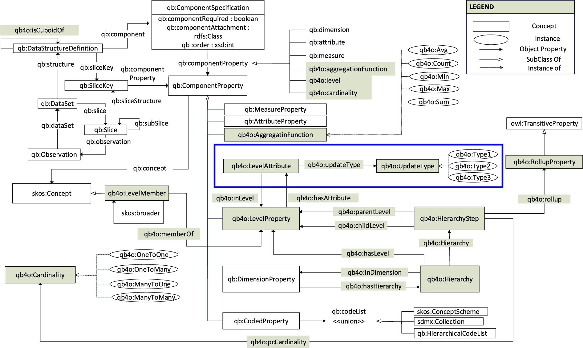
In QB4OLAP, the concept qb:DataSet is used to define a dataset of observations. The structure of the dataset is defined using the concept qb:DataStructureDefinition. The structure can be a cube (if it is defined in terms of dimensions and measures) or a cuboid (if it is defined in terms of lower levels of the dimensions and measures). The property qb4o:isCuboidOf is used to relate a cuboid to its corresponding cube. To define dimensions, levels and hierarchies, the concepts qb4o:DimensionProperty, qb4o:LevelProperty, and qb4o:Hierarchy are used. A dimension can have one or more hierarchies. The relationship between a dimension and its hierarchies are connected via the qb4o:hasHierarchy property or its inverse property qb4o:inHierarchy. Conceptually, a level may belong to different hierarchies; therefore, it may have one or more parent levels. Each parent and child pair has a cardinality constraint (e.g., 1-1, n-1, 1-n, and n-n) [62]. To allow this kind of complex nature, hierarchies in QB4OLAP are defined as a composition of pairs of levels, which are represented using the concept qb4o:HierarchyStep. Each hierarchy step (pair) is connected to its component levels using the properties qb4o:parentLevel and qb4o:childLevel. A roll-up relationship between two levels are defined by creating a property which is an instance of the concept qb4o:RollupProperty; each hierarchy step is linked to a roll-up relationship with the property qb4o:rollup and the cardinality constraint of that relationship is connected to the hierarchy step using the qb4o:pcCardinality property. A hierarchy step is attached to the hierarchies it belongs to using the property qb4o:inHierarchy [19]. The concept qb4o:LevelAttributes is used to define attributes of levels. We extend this QB4OLAP ontology (the blue-colored box in the figure) to enable different types of dimension updates (Type 1, Type 2, and Type 3) to accommodate dimension update in an SDW, which are defined by Ralph Kimball in [37]. To define the update-type of a level attribute in the TBox level, we introduce the qb4o:UpdateType class whose instances are qb4o:Type1, qb4o:Type2, and qb4o:Type3. A level attribute is connected to its update-type by the property qb4o:updateType. The level attributes are linked to its corresponding levels using the property qb4o:hasAttribute. We extend the definition of C and P of a TBox, T for an SDW as
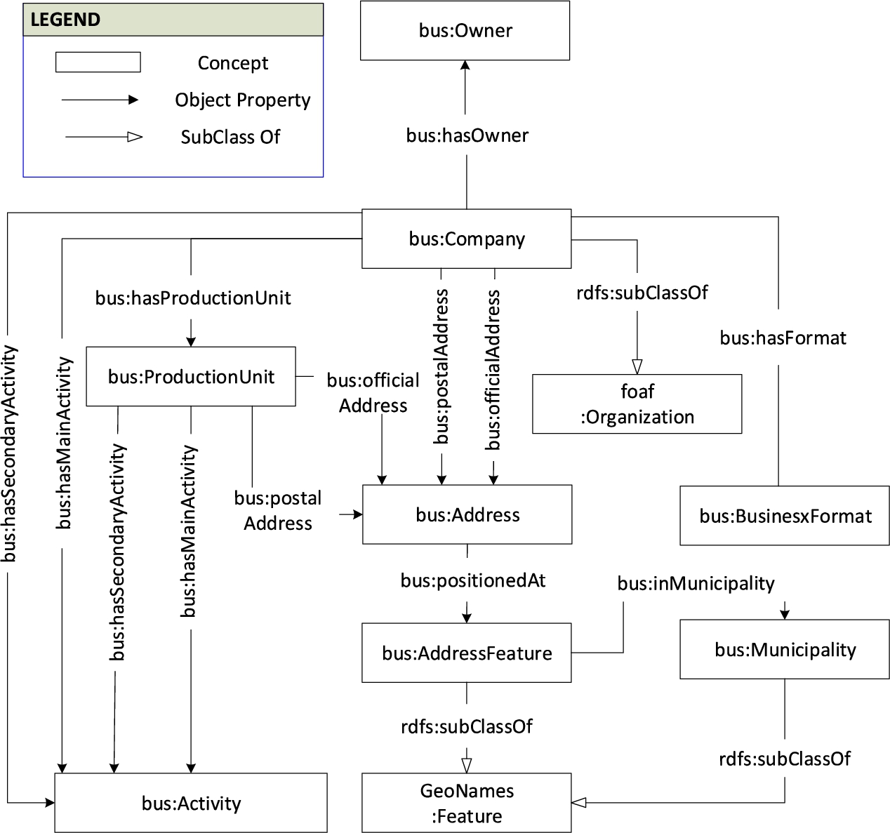
Fig. 2.
The ontology of the Danish Business dataset. Due to the large number of datatype properties, they are not included.
3.A use case
We create a semantic Data Warehouse (SDW) by integrating two data sources, namely, a Danish Agriculture and Business knowledge base and an EU Farm Subsidy dataset. Both data sources are described below.
Description of Danish Agriculture and Business knowledge base The Danish Agriculture and Business knowledge base integrates a Danish Agricultural dataset and a Danish Business dataset. The knowledge base can be queried through the SPARQL endpoint http://extbi.lab.aau.dk:8080/sparql/. In our use case, we only use the business related information from this knowledge base and call it the Danish Business dataset (DBD). The relevant portion of the ontology of the knowledge base is illustrated in Fig. 2. Generally, in an ontology, a concept provides a general description of the properties and behavior for the similar type of resources; an object property relates among the instances of concepts; a data type property is used to associate the instances of a concept to literals.
We start the description from the concept bus:Owner. This concept contains information about the owners of companies, the type of the ownership, and the start date of the company ownership. A company is connected to its owner through the bus:hasOwner property. The bus:Company concept is related to bus:BusinessFormat and bus:ProductionUnit through the bus:hasProductionUnit and bus:hasFormat properties. Companies and their production units have one or more main and secondary activities. Each company and each production unit has a postal address and an official address. Each address is positioned at an address feature, which is in turn contained within a particular municipality.
Description of the EU subsidy dataset Every year, the European Union provides subsidies to the farms of its member countries. We collect EU Farm subsidies for Denmark from https://data.farmsubsidy.org/Old/. The dataset contains two MS Access database tables: Recipient and Payment. The Recipient table contains the information of recipients who receive the subsidies, and the Payment table contains the amount of subsidy given to the recipients. We create a semantic version of the dataset using SETLPROG framework [43]. We call it the Subsidy dataset. At first, we manually define an ontology, to describe the schema of the dataset, and the mappings between the ontology and database tables. Then, we populate the ontology with the instances of the source database files. Figure 3 shows the ontology of the Subsidy dataset.
Fig. 3.
The ontology of the Subsidy dataset. Due to the large number of datatype properties, all are not included.
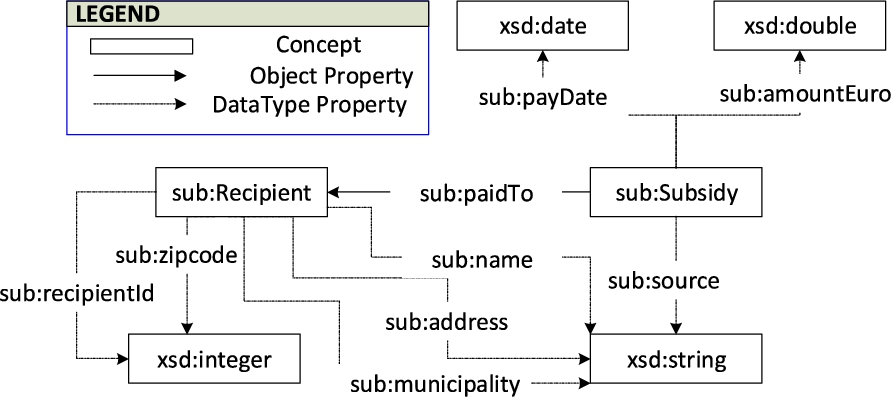
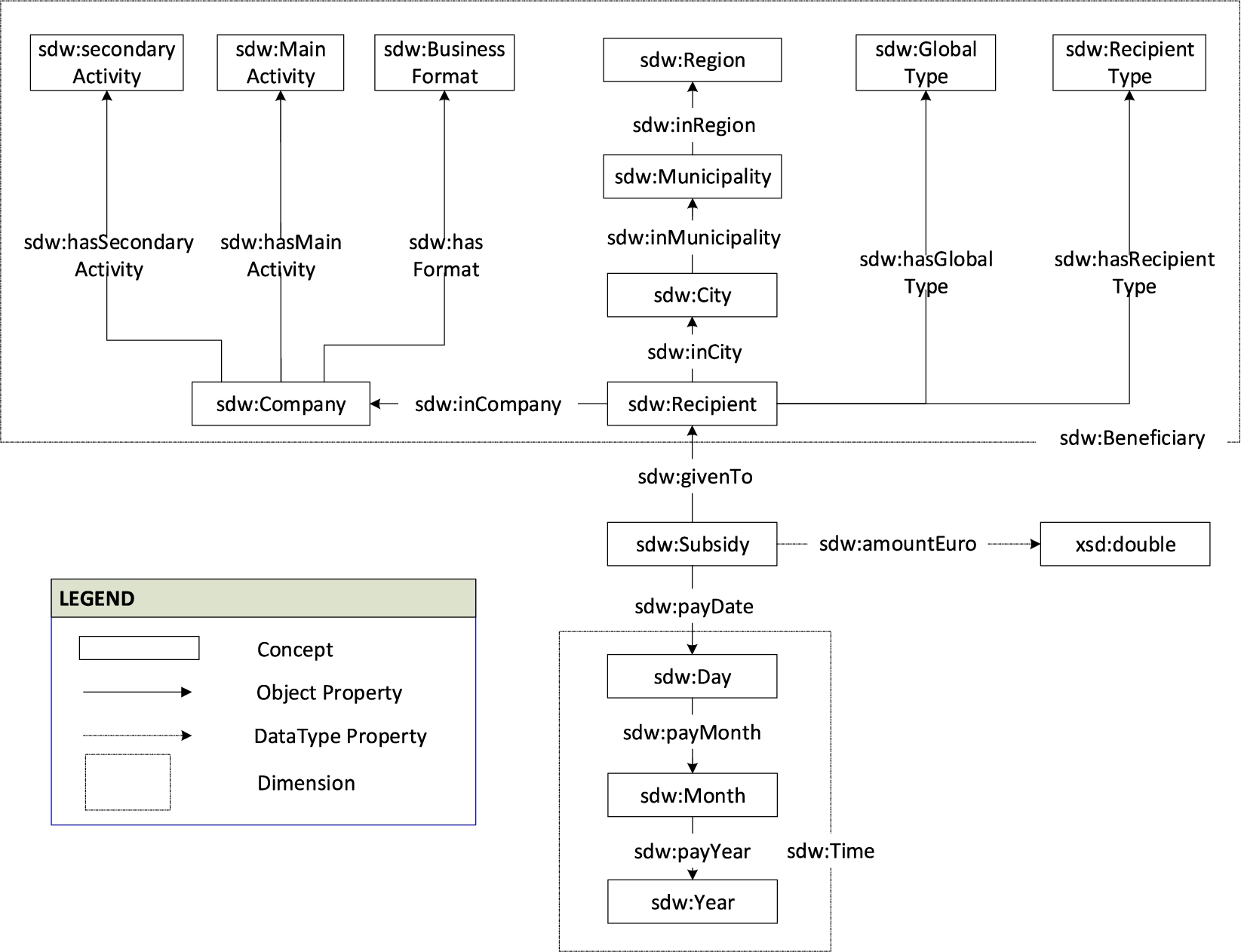
Fig. 4.
The ontology of the MD SDW. Due to the large number, data properties of the dimensions are not shown.
Example 1.
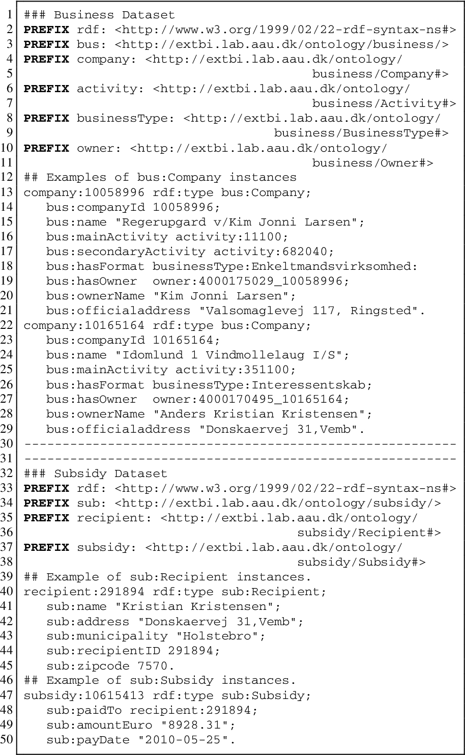
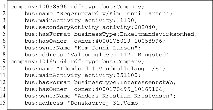
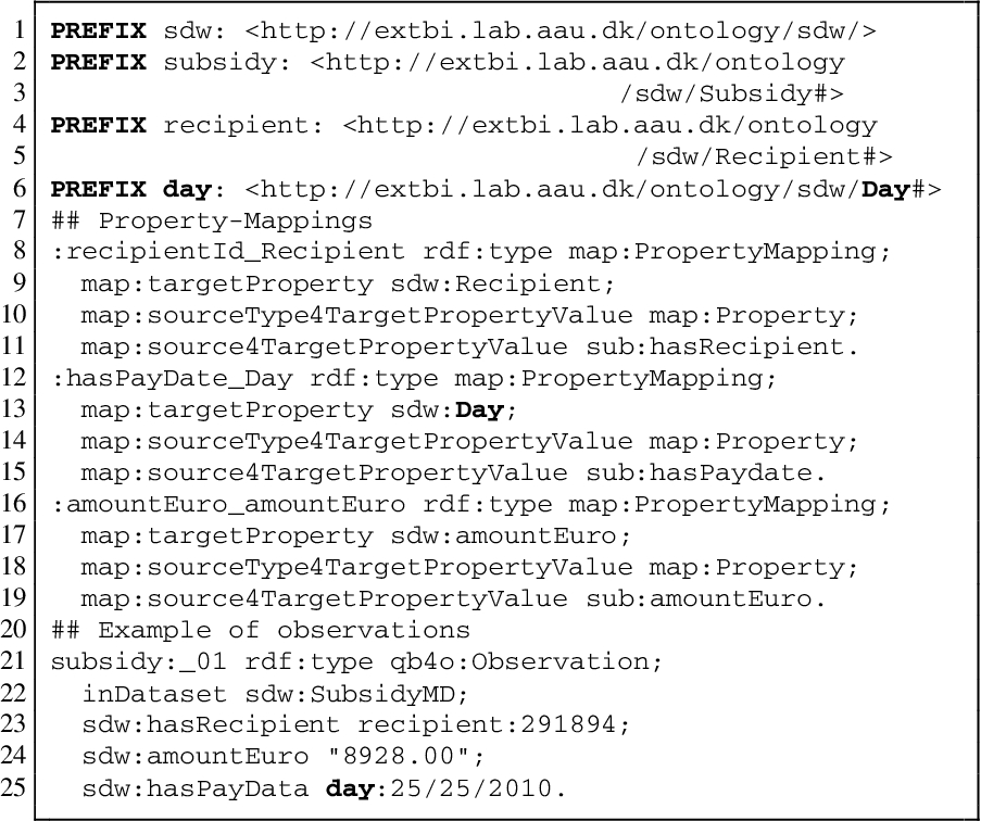
Listing 1 shows the example instances of bus:Company from the Danish Business dataset and sub:Recipient and sub:Subsidy from the EU Subsidy dataset.
Listing 1.
Example instances of the DBD and the Subsidy dataset
Description of the Semantic Data Warehouse Our goal is to develop an MD Semantic Data Warehouse (SDW) by integrating the Subsidy and the DBD datasets. The sub:Recipient concept in the Subsidy dataset contains the information of recipient id, name, address, etc. From bus:Company in the DBD, we can extract information of an owner of a company who received the EU farm subsidies. Therefore, we can integrate both DBD and Subsidy datasets. The ontology of the MD SDW to store EU subsidy information corresponding to the Danish companies is shown in Fig. 4, where the concept sdw:Subsidy represents the facts of the SDW. The SDW has two dimensions, namely sdw:Benificiary and sdw:Time. The dimensions are shown by a box with dotted-line in Fig. 4. Here, each level of the dimensions are represented by a concept, and the connections among levels are represented through object properties.
4.Overview of the integration process
Fig. 5.
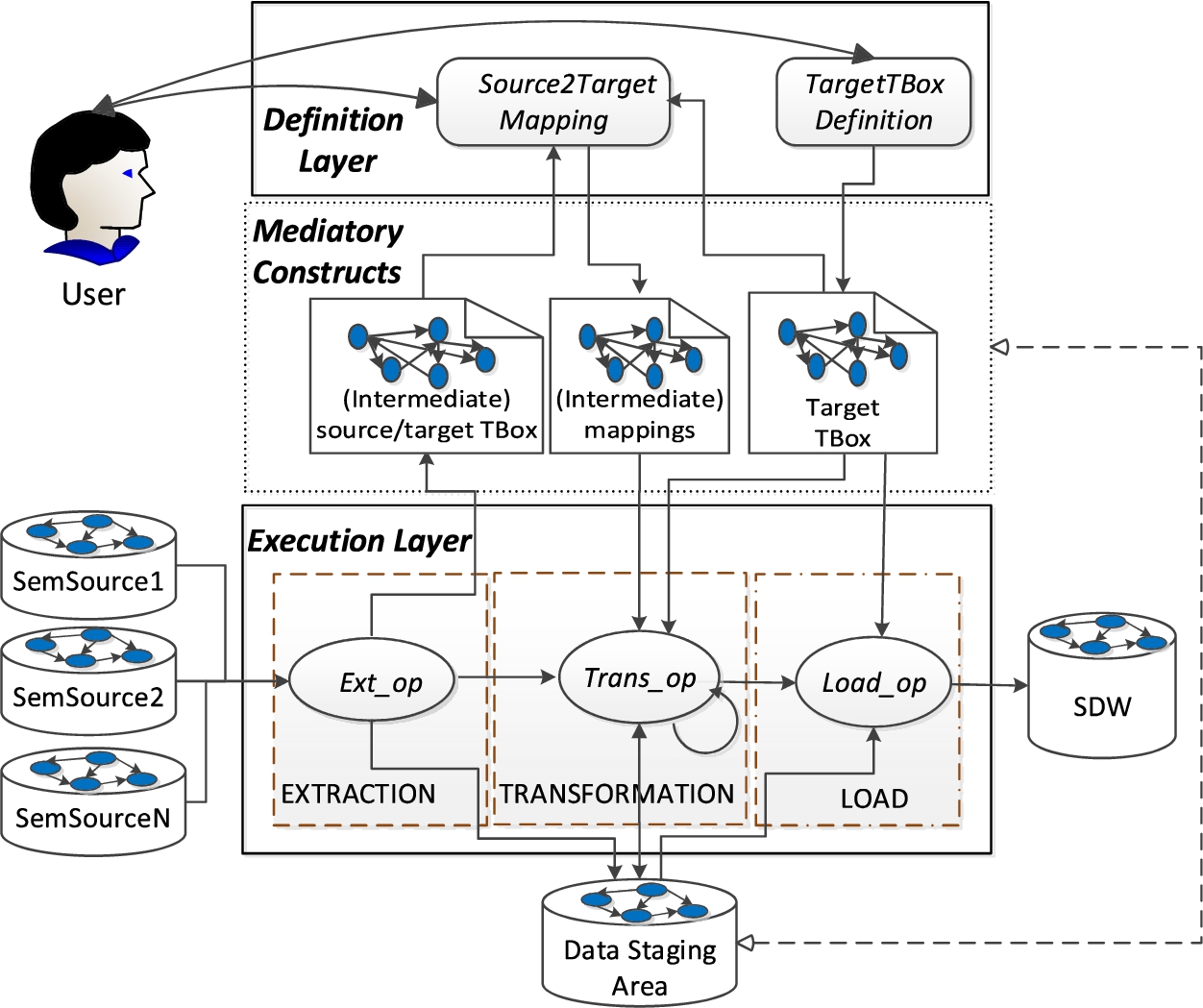
The overall semantic data integration process. Here, the round-corner rectangle, data stores, dotted boxes, ellipses, and arrows indicate the tasks, semantic data sources and SDW, the phases of the ETL process, ETL operations and flow directions.
In this paper, we assume that all given data sources are semantically defined and the goal is to develop an SDW. The first step of building an SDW is to design its TBox. There are two approaches to design the TBox of an SDW, namely source-driven and demand-driven [61]. In the former, the SDW’s TBox is obtained by analyzing the sources. Here, ontology alignment techniques [40] can be used to semi-automatically define the SDW. Then, designers can identify the multidimensional constructs from the integrated TBox and annotate them with the QB4OLAP vocabulary. In the latter, SDW designers first identify and analyze the needs of business users as well as decision makers, and based on those requirements, they define the target TBox with multidimensional semantics using the QB4OLAP vocabulary. How to design a Target TBox is orthogonal to our approach. Here, we merely provide an interface to facilitate creating it regardless of whatever approach was used to design it.
Table 1
Summary of the ETL operations
| Operation category | Operation name | Compatible successors | Objectives |
| Extraction | GraphExtractor | GraphExtractor, TBoxExtraction, TransformationOnLiteral, JoinTransformation, LevelMemberGenerator, ObservationGenerator, DataChangeDetector, UpdateLevel, Loader | It retrieves an RDF graph in terms of RDF triples from semantic data sources. |
| Transformation | TBoxExtraction | It derives a TBox from a given ABox. | |
| TransformationOnLiteral | TransformationOnLiteral, JoinTransformation, LevelMemberGenerator, ObservationGenerator, Loader | It transforms the source data according to the expressions described in the source-to-target mapping. | |
| JoinTransformation | TransformationOnLiteral, JoinTransformation, LevelMemberGenerator, ObservationGenerator, Loader | It joins two data sources and transforms the data according to the expressions described in the source-to-target mapping. | |
| LevelMemberGenerator (QB4OLAP construct) | Loader | It populates levels of the target with the input data. | |
| ObservationGenerator (QB4OLAP construct) | Loader | It populates facts of the target with the input data. | |
| DataChangeDetector | LevelMemberGenerator, UpdateLevel | It returns the differences between the new source dataset and the old one. | |
| UpdateLevel | Loader | It reflects the changes occurred in the source data to the target level. | |
| MaterializeInference | Loader | It enriches the SDW by materializing the inferred triples. | |
| ExternalLinking | Loader | It links internal resources with external KBs. | |
| Load | Loader | It loads the data into the SDW. |
After creating the TBox of the SDW, the next step is to create the ETL process. ETL is the backbone process by which data are entered into the SDW and the main focus of this paper. The ETL process is composed of three phases: extraction, transformation, and load. A phase is a sub-process of the ETL which provides a meaningful output that can be fed to the next phase as an input. Each phase includes a set of operations. The extraction operations extract data from the data sources and make it available for further processing as intermediate results. The transformation operations are applied on intermediate results, while the load operations load the transformed data into the DW. The intermediate results can be either materialized in a data staging area or kept in memory. A data staging area (temporary) persists data for cleansing, transforming, and future use. It may also prevent the loss of extracted or transformed data in case of the failure of the loading process.
As we want to separate the metadata needed to create ETL flows from their execution, we introduce a two-layered integration process, see Fig. 5. In the Definition Layer, a single source of metadata truth is defined. This includes: the target SDW, semantic representation of the source schemas, and a source to target mapping file. Relevantly, the metadata created represents the ETL flow at the schema level. In the Execution Layer, ETL data flows based on high-level operations are created. This layer executes the ETL flows for instances (i.e., at the data level). Importantly, each ETL operation is fed the metadata created to parameterize themselves automatically. Additionally, the Execution Layer automatically checks the correctness of the created flow, by checking the compatibility of the output and input of consecutive operators. Overall the data integration process requires the following four steps in the detailed order.
1. Defining the target TBox with MD semantics using QB and QB4OLAP constructs. In addition, the TBox can be enriched with RDFS/OWL concepts and properties. However, we do not validate the correctness of the added semantics beyond the MD model. This step is done at the Definition Layer.
2. Extracting source TBoxes from the given sources. This step is done at the Definition Layer.
3. Creating mappings among source and target constructs to characterize ETL flows. The created mappings are expressed using the proposed S2TMAP vocabulary. This step is also done at the Definition Layer.
4. Populating the ABox of the SDW implementing ETL flows. This step is done at the Execution Layer.
Since traditional ETL tools (e.g., PDI) do not have ETL operations supporting the creation of an SDW, we propose a set of ETL operations for each phase of the ETL to process semantic data sources. The operations are categorized based on their functionality. Table 1 summarizes each operation with its corresponding category name, compatible successors, and its objectives. Next, we present the details of each construct of the layers presented in Fig. 5.
5.The definition layer
This layer contains two tasks (TargetTBoxDefinition and Source2TargetMapping) and one operation TBoxExtraction. The semantics of the tasks are described below.
TargetTBoxDefinition The objective of this task is to define a target TBox with MD semantics. There are two main components of the MD structure: dimensions and cubes. To formally define the schema of these components, we use the notation from [12] with some modifications.
Definition 1.
A dimension schema can formally be defined as a 5-tuple
–
–
– → is a strict partial order on
–
–
Example 2.
Figure 4 shows that our use case MD SDW has two dimensions: sdw:Time and sdw:Beneficiary. The dimension schema of sdw:Time is formally defined as follows:
1.
2.
3.
4.
5.
Definition 2.
A cube schema is a 4-tuple
–
–
–
–
Example 3.
The cube schema of our use case, shown in Fig. 4, is formally defined as follows:
1.
2.
3.
4.
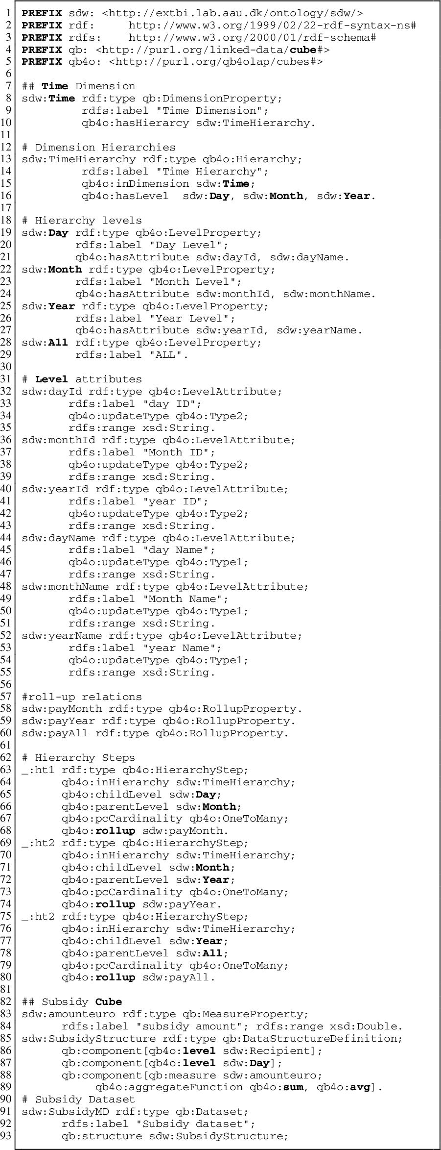
In Section 2.3, we discussed how the QB4OLAP vocabulary is used to define different constructs of an SDW. Listing 2 represents the sdw:Time dimension and sdw:Subsidy cube in QB4OLAP.
Listing 2.
QB4OLAP representation of sdw:Time dimension and sdw:Subsidy cube
TBoxExtraction After defining a target TBox, the next step is to extract source TBoxes. Typically, in a semantic source, the TBox and ABox of the source are provided. Therefore, no external extraction task/operation is required. However, sometimes, the source contains only the ABox, no TBox. In that scenario, an extraction process is required to derive a TBox from the ABox. Since the schema level mappings are necessary to create the ETL process, and the ETL process will extract data from the ABox, we only consider the intentional knowledge available in the ABox in the TBox extraction process. We formally define the process as follows.
Definition 3.
The TBox extraction operation from a given ABox, ABox is defined as
1. C: By checking the unique objects of the triples in ABox where rdf:type is used as a predicate, C is identified.
2. H: The taxonomies among concepts are identified by checking the instances they share among themselves. Let
3. P, D, R: By checking the unique predicates of the triples, P is derived. A property
Note that proving the formal correctness of the approach is beyond the scope of this paper and left for future work.
SourceToTargetMapping Once the target and source TBoxes are defined, the next task is to characterize the ETL flows at the Definition Layer by creating source-to-target mappings. Because of the heterogeneous nature of source data, mappings among sources and the target should be done at the TBox level. In principle, mappings are constructed between sources and the target; however, since mappings can get very complicated, we allow to create a sequence of SourceToTargetMapping definitions whose subsequent input is generated by the preceding operation. The communication between these operations is by means of a materialized intermediate mapping definition and it is meant to facilitate the creation of very complex flows (i.e., mappings) between source and target.
A source-to-target mapping is constructed between a source and a target TBox, and it consists of a set of concept-mappings. A concept-mapping defines i) a relationship (equivalence, subsumption, supersumption, or join) between a source and the corresponding target concept, ii) which source instances are mapped (either all or a subset defined by a filter condition), iii) the rule to create the IRIs for target concept instances, iv) the source and target ABox locations, v) the common properties between two concepts if their relationship is join, vi) the sequence of ETL operations required to process the concept-mapping, and vii) a set of property-mappings for the properties having the target concept as a domain. A property-mapping defines how a target property is mapped from either a source property or an expression over properties. Definition 4 formally defines a source-to-target mapping.
Definition 4.
Let
The semantics of each concept-mapping tuple is given below.
–
–
 represents the relationship between the source and target concept. The relationship can be either
 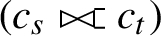 , or a left-outer join
 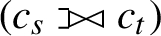 . A join relationship exists between two sources when there is a need to populate a target element (a level, a (QB) dataset, or a concept) from multiple sources. Since a concept-mapping represents a binary relationship, to join n sources, an ETL process requires
 –
–
–
–
–
–
In principle, an SDW is populated from multiple sources, and a source-to-target ETL flow requires more than one intermediate concept-mapping definitions. Therefore, a complete ETL process requires a set of source-to-target mappings. We say a mapping file is a set of source-to-target mappings. Definition 5 formally defines a mapping file.
Definition 5.
Fig. 6.
Graphical overview of key terms and their relationships to the S2TMAP vocabulary.
To implement the source-to-target mappings formally defined above, we propose an OWL-based mapping vocabulary: Source-to-Target Mapping (S2TMAP). Figure 6 depicts the mapping vocabulary. A mapping between a source and a target TBox is represented as an instance of the concept map:MapDataset. The source and target TBoxes are defined by instantiating map:TBox, and these TBoxes are connected to the mapping dataset using the properties map:sourceTBox and map:targetTBox, respectively. A concept-mapping (an instance of map:ConceptMapping) is used to map between a source and a target concepts (instances of map:Concept). A concept-mapping is connected to a mapping dataset using the map:mapDataset property. The source and target ABox locations of the concept-mapping are defined through the map:sourceLocation and map:targetLocation properties. The relationship between the concepts can be either map:subsumption, map:supersumption, map:Join, map:LeftJoin, map:RightJoin, or map:Equivalence, and it is connected to the concept-mapping via the map:relation property. The sequence of ETL operations, required to implement the concept-mapping at the ABox level, is defined through an RDF sequence. To express joins, the source and target concept in a concept-mapping represent the concepts to be joined, and the join result is stored in the target concept as an intermediate result. In a concept-mapping, we, via map:commonProperty, identify the join attributes with a blank node (instance of map:CommonProperty) that has, in turn, two properties identifying the source and target join attributes; i.e., map:commonSourceProperty and map:commonTargetProperty. Since a join can be defined on multiple attributes, we may have multiple blank node definitions. The type of target instance IRIs is stated using the property map:TargetInstanceIRIType. If the type is either map:Property or map:Expression, then the property or expression, to be used to generate the IRIs, is given by map:targetInstanceIRIvalue.
To map at the property stage, a property-mapping (an instance of map:PropertyMapping) is used. The association between a property-mapping and a concept-mapping is defined by map:conceptMapping. The target property of the property-mapping is stated using map:targetProperty, and that target property can be mapped with either a source property or an expression. The source type of target property is determined through map:sourceType4TargetProperty property, and the value is defined by map:source4TargetPropertyValue.
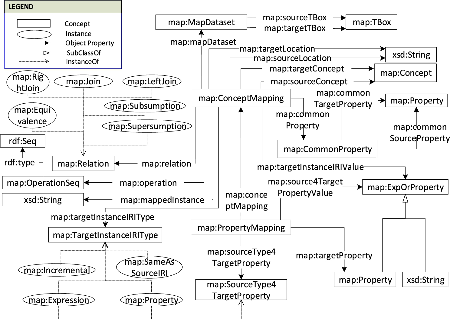
Example 4.
Listing 3 represents a snippet of the mapping file of our use case MD SDW and the source datasets. In the Execution Layer, we show how the different segments of this mapping file will be used by each ETL operation.
Listing 3.
An S2TMAP representation of the mapping file of our use case
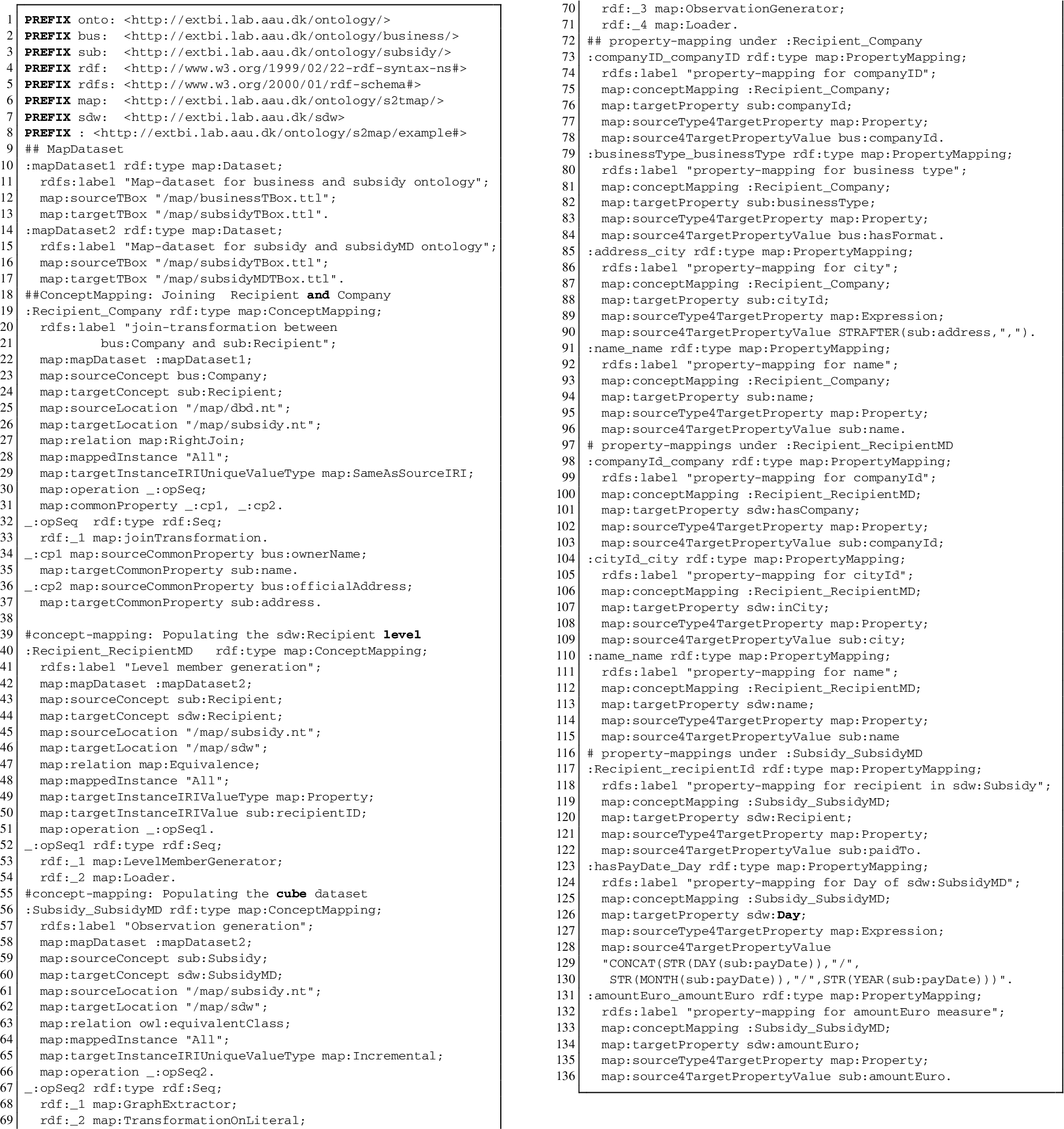
A mapping file is a Directed Acyclic Graph (DAG). Figure 7 shows the DAG representation of Listing 3. In this figure, the sources, intermediate results and the SDW are denoted as nodes of the DAG and edges of the DAG represent the operations. The dotted-lines shows the parts of the ETL covered by concept-mappings, represented by a rectangle.
6.The Execution Layer
In the Execution Layer, ETL data flows are constructed to populate an MD SDW. Table 1 summarizes the set of ETL operations. In the following, we present an overview of each operation category-wise. Here, we give the intuitions of the ETL operations in terms of definitions and examples. To reduce the complexity and length of the paper, we place the formal semantics of the ETL operations in the Appendix. In this section, we only present the signature of each operation. That is, the main inputs required to execute the operation. As an ETL data flow is a sequence of operations and an operation in the sequence communicates with its preceding and subsequent operations by means of materialized intermediate results, all the operations presented here have side effects55 instead of returning output.
Developers can use either of the two following options: (i) The recommended option is that given a TBox construct aConstruct (a concept, a level, or a QB dataset) and a mapping file aMappings generated in the Definition Layer, the automatic ETL execution flow generation process will automatically extract the parameter values from aMappings (see Section 7 for a detailed explanation of the automatic ETL execution flow generation process). (ii) They can manually set input parameters at the operation level. In this section, we follow the following order to present each operation: 1) we first give a high-level definition of the operation; 2) then, we define how the automatic ETL execution flow generation process parameterizes the operation from the mapping file, and 3) finally, we present an example showing how developers can manually parameterize the operation. When introducing the operations and referring to their automatic parametrization, we will refer to aMappings and aConstruct as defined here. Note that each operation is bound to exactly one concept-mapping at a time in the mapping file (discussed in Section 7).
6.1.Extraction operations
Extraction is process of data retrieval from the sources. Here, we introduce two extraction operations for semantic sources: (i) GraphExtractor – to form/extract an RDF graph from a semantic source and (ii) TBoxExtraction – to derive a TBox from a semantic source as described in Section 5. As such, TBoxExtraction is the only operation in the Execution Layer generating metadata stored in the Mediatory Constructs (see Fig. 5).
GraphExtractor(Q, G, outputPattern, tABox) Since the data integration process proposed in this paper uses RDF as the canonical model, we extract/generate RDF triples from the sources with this operation. GraphExtractor is functionally equivalent to SPARQL CONSTRUCT queries [39].
If the ETL execution flow is generated automatically, the automatic ETL execution flow generation process first identifies the concept-mapping cm from aMappings where aConstruct appears (i.e., in aMapping,
Example 5.
Listing 1 shows the example instances of the Danish Business Dataset (DBD). To extract all instances of bus:Company from the dataset, we use the GraphExtractor(Q, G, outputPattern, tABox) operation, where
Listing 4.
Example of GraphExtractor
TBoxExtraction is already described in Section 5, therefore, we do not repeat it here.
6.2.Transformation operations
Transformation operations transform the extracted data according to the semantics of the SDW. Here, we define the following semantic-aware ETL transformation operations: TransformationOnLiteral, JoinTransformation, LevelMemberGenerator, ObservationGenerator, ChangedDataCapture, UpdateLevel, External linking, and MaterializeInference. The following describe each operation.
TransformationOnLiteral(sConstruct, tConstruct, sTBox, sABox propertyMappings, tABox) As described in the SourceToTargetMapping task, a property (in a property-mapping) of a target construct (i.e., a level, a QB dataset, or a concept) can be mapped to either a source concept property or an expression over the source properties. An expression allows arithmetic operations, datatype (string, number, and date) conversion and processing functions, and group functions (sum, avg, max, min, count) as defined in SPARQL [25]. This operation generates the instances of the target construct by resolving the source expressions mapped to its properties.
If the ETL execution flow is generated automatically, the automatic ETL execution flow generation process first identifies the concept-mapping
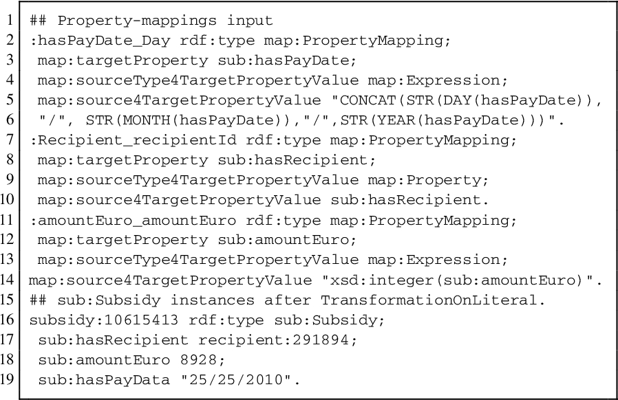
Example 6.
Listing 5 (lines 16–19) shows the transformed instances after applying the operation TransformationOnLiteral(sConstruct, tConstruct, sTBox, sABox, PropertyMappings, tABox), where
Listing 5.
Example of TransformationOnLiteral
JoinTransformation(sConstruct, tConstruct, sTBox, tTBox, sABox, tABox, comProperty, propertyMappings) A TBox construct (a concept, a level, or a QB dataset) can be populated from multiple sources. Therefore, an operation is necessary to join and transform data coming from different sources. Two constructs of the same or different sources can only be joined if they share some common properties. This operation joins a source and a target constructs based on their common properties and produce the instances of the target construct by resolving the source expressions mapped to target properties. To join n sources, an ETL process requires n-1 JoinTransformation operations.
If the ETL execution flow is generated automatically, the automatic ETL execution flow generation process first identifies the concept-mapping cm from aMappings, where aConstruct appears and the operation to process
A developer can also manually set the parameters. Once it is parameterized, JoinTransformation joins two constructs based on comProperty, transforms their data based on the expressions (specified through map:source4TargetPropertyValue) defined in propertyMappings, and updates tABox based on the join result. It creates a SPARQL SELECT query joining two constructs using either AND or OPT features, and on top of that query, it forms a SPARQL CONSTRUCT query to generate the transformed tABox.
Example 7.
The recipients in sdw:Recipient need to be enriched with their company information available in the Danish Business dataset. Therefore, a join operation is necessary between sub:Recipient and bus:Company. The concept-mapping of this join is described in Listing 3 at lines 19–37. They are joined by two concept properties: recipient names and their addresses (lines 31, 34–37). We join and transform bus:Company and sub:Recipient using JoinTransformation(sConstruct, tConstruct, sTBox, tTBox, sABox, tABox, comProperty, propertyMappings), where
1. sConstruct= bus:Company,
2. tConstruct= sub:Recipient,
3. sTBox= “/map/businessTBox.ttl”,
4. tTBox= “/map/subsidyTBox.ttl”,
5. sABox= source instances of bus:Company (lines 13–29 in Listing 1),
6. tABox= source instances of sub:Recipient (lines 40–45 in Listing 1),
7. comProperty = lines 31, 34–37 in Listing 3,
8. propertyMappings = lines 73–96 in Listing 3.
Listing 6.
Example of JoinTransformation
LevelMemberGenerator(sConstruct, level, sTBox, sABox, tTBox, iriValue, iriGraph, propertyMappings, tABox) In QB4OLAP, dimensional data are physically stored in levels. A level member, in an SDW, is described by a unique IRI and its semantically linked properties (i.e., level attributes and roll-up properties). This operation generates data for a dimension schema defined in Definition 1.
If the ETL execution flow is generated automatically, the automatic process first identifies the concept-mapping cm from aMappings, where aConstruct appears and the operation to process cm is LevelMemberGenerator. Then it parameterizes LevelMemberGenerator as follows: 1) sConstruct is the source construct defined by map:sourceConcept; 2) level is the target level88 defined by the map:targetConcept property; 3) sTBox and tTBox are the source and target TBoxes of cm’s map dataset, defined by the properties map:sourceTBox and map:targetTBox; 4) sABox is the source ABox defined by the property map:sourceLocation; 5) iriValue is a rule99 to create IRIs for the level members and it is defined defined by the map:TargetInstanceIriValue property; 6) iriGraph is the IRI graph1010 within which to look up IRIs, given by the developer in the automatic ETL flow generation process; 7) propertyMappings is the set of property-mappings defined under cm; and 8) tABox is the target ABox location defined by map:targetLocation.
A developer can also manually set the paramenters. Once it is parameterized, LevelMemberGenerator operation generates QB4OLAP-compliant triples for the level members of level based on the semantics encoded in tTBox and stores them in tABox.
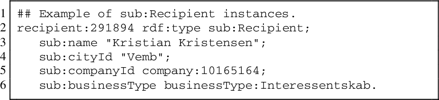
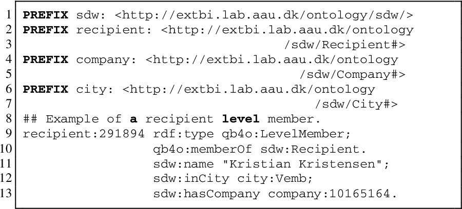
Example 8.
Listing 3 shows a concept-mapping (lines 40–54) describing how to populate sdw:Recipient from sub:Recipient. Listing 7 shows the level member created by the LevelMemberGenerator(level, tTBox, sABox, iriValue, iriGraph, propertyMappings, tABox) operation, where
1. sConstruct= sub:Recipient,
2. level= sdw:Recipient,
3. sTBox= “/map/subsidyTBox.ttl”,
4. sABox= “/map/subsidy.ttl”, shown in Example 7,
5. tTBox = “/map/subsidyMDTBox.ttl”,
6. iriValue = sub:recipientID,
7. iriGraph = “/map/provGraph.nt”,
8. propertyMappings= lines 98–115 in Listing 3,
9. tABox=”/map/temp.ttl”.
Listing 7.
Example of LevelMemberGenerator
ObservationGenerator(sConstruct, dataset, sTBox, sABox, tTBox, iriValue, iriGraph, propertyMappings, tABox) In QB4OLAP, an observation represents a fact. A fact is uniquely identified by an IRI, which is defined by a combination of several members from different levels and contains values for different measure properties. This operation generates data for a cube schema defined in Definition 2.
If the ETL execution flow is generated automatically, the way used by the automatic ETL execution flow generation process to extract values for the parameters of ObservationGenerator from aMappings is analogous to LevelMemberGenerator. Developers can also manually set the parameters. Once it is parameterized, the operation generates QB4OLAP-compliant triples for observations of the QB datasetdataset based on the semantics encoded in tTBox and stores them in tABox.
Example 9.
Listing 8 (lines 21–25) shows a QB4OL-AP-compliant observation create by the ObservationGenerator(sConstruct, dataset, sTBox, sABox, tTBox, iriValue, iriGraph, propertyMappings, tABox) operation, where
1. sConstruct = sub:Subsidy,
2. dataset = sdw:SubsidyMD,
3. sTBox = “/map/subsidyTBox.ttl”
4. sABox = “/map/subsidy.ttl”, shown in Example 6,
5. tTBox = “/map/subsidyMDTBox.ttl”, shown in Listing 2,
6. iriValue = “Incremental”,
7. iriGraph = “/map/provGraph.nt”,
8. propertyMappings = lines 8–19 in Listing 8,
9. tABox = “/map/temp2.ttl”.
Listing 8.
Example of ObservationGenerator
ChangedDataCapture(nABox, oABox, flag) In a real-world scenario changes occur in a semantic source both at the schema and instance level. Therefore, an SDW needs to take action based on the changed schema and instances. The adaption of the SDW TBox with the changes of source schemas is an analytical task and requires the involvement of domain experts, therefore, it is out of the scope of this paper. Here, only the changes at the instance level are considered.
If the ETL execution flow is generated automatically, the automatic process first identifies the concept-mapping cm from aMappings, where aConstruct appears and the operation to process cm is ChangedDataCapture. Then, it takes map:sourceLocation and map:targetLocation for nABox (new dimensional instances in a source) and oABox (old dimensional instances in a source), respectively, to parametrize this operation. flag depends on the next operation in the operation sequence.
Developers can also manually set the parameters. From the given inputs, ChangedDataCapture outputs either 1) a set of new instances (in the case of SDW evolution, i.e.,
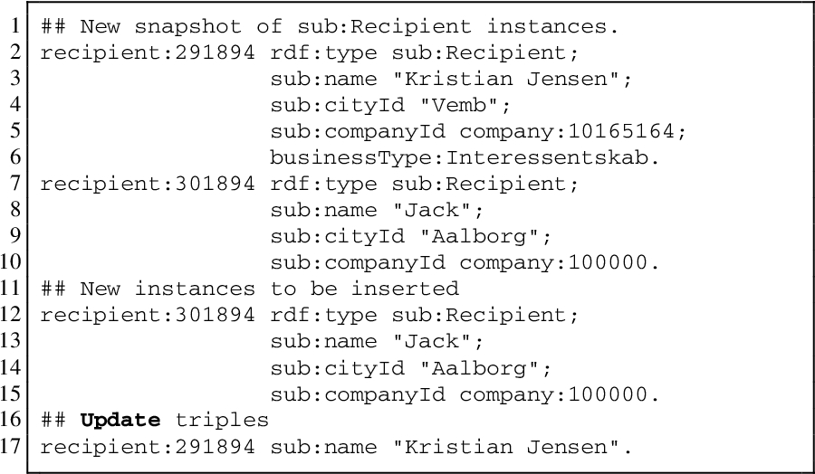
Example 10.
Suppose Listing 6 is the old ABox of sub:Recipient and the new ABox is at lines 2–10 in Listing 9. This operation outputs either 1) the new instance set (in this case, lines 12–15 in the listing) or 2) the updated triples (in this case, line 17).
Listing 9.
Example of ChangedDataCapture
UpdateLevel(level, updatedTriples, sABox, tTBox, tABox, propertyMappings, iriGraph) Based on the triples updated in the source ABox sABox for the level level (generated by ChangedDataCapture), this operation updates the target ABox tABox to reflect the changes in the SDW according to the semantics encoded in the target TBox tTBox and level property-mappings propertyMappings. Here, we address three update types (Type1-update, Type2-update, and Type3-update), defined by Ralph Kimball in [37] for a traditional DW, in an SDW environment. The update types are already defined in tTBox for each level attribute of level (as discussed in Section 2.3), so they do not need to be provided as parameters. As we consider only instance level updates, only the objects of the source updated triples are updated. To reflect a source updated triple in level, the level member using the triple to describe itself, will be updated. In short, the level member is updated in the following three ways: 1) A Type1-update simply overwrites the old object with the current object. 2) A Type2-update creates a new version for the level member (i.e., it keeps the previous version and creates a new updated one). It adds the validity interval for both versions. Further, if the level member is a member of an upper level in the hierarchy of a dimension, the changes are propagated downward in the hierarchy, too. 3) A Type3-update overwrites the old object with the new one. Besides, it adds an additional triple for each changed object to keep the old object. The subject of the additional triple is the instance IRI, the object of the triple is the old object, and the predicate is concat(oldPredicate, “oldValue”).
If the ETL execution flow is generated automatically, this operation first identifies the concept-mapping cm from aMappings, where aConstruct appears and the operation to process cm is UpdateLevel. Then it parameterizes LevelMemberGenerator as follows: 1) level is defined by the map:targetConcept; 2) sABox is old source data; 3) updatedTriples is the source location defined by map:sourceLocation; 4) tTBox is the target TBox of cm’s map-dataset, defined by the property map:targetTBox; 5) tABox is defined by map:targetLocation; 6) propertyMappings is the set of property-mappings defined under cm; and 7) iriGraph is given by developer in the automatic ETL flow generation process.
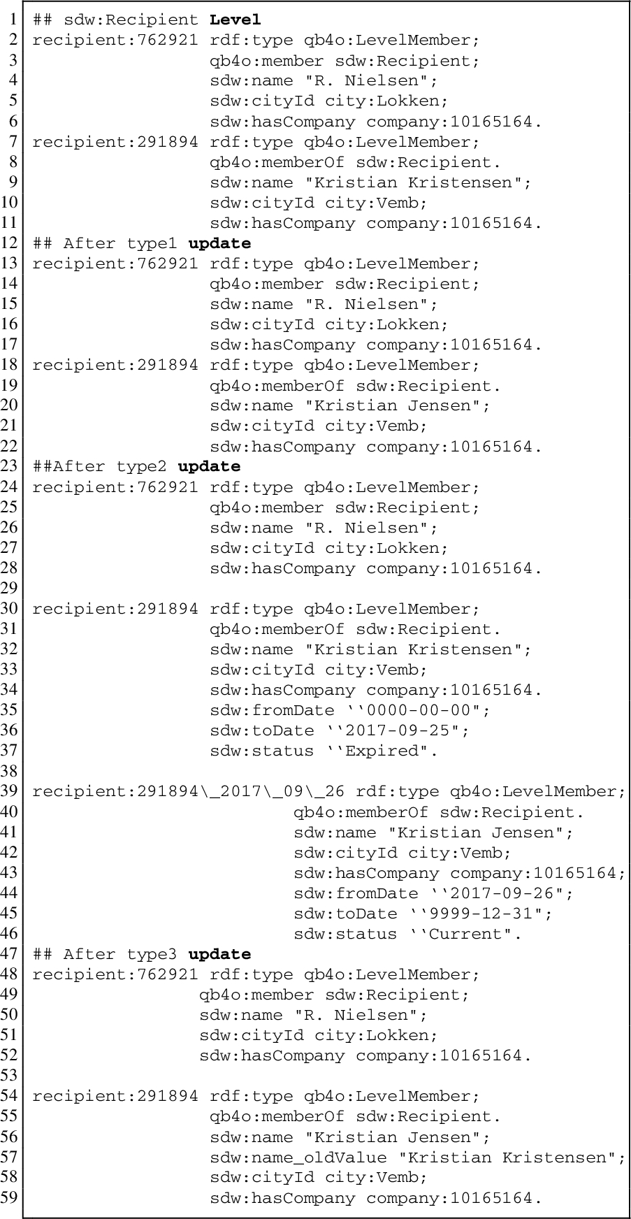
Example 11.
Listing 10 describes how different types of updates work by considering two members of the sdw:Recipient level (lines 2–11). As the name of the second member (lines 7–11) is changed to “Kristian Jensen” from “Kristian Kristensen”, as found in Listing 9. A Type1-update simply overwrites the existing name (line 20). A Type2-update creates a new version (lines 39–46). Both old and new versions contain validity interval (lines 35–37) and (lines 44–46). A Type3-Update overwrites the old name (line 56) and adds a new triple to keep the old name (line 57).
Listing 10.
Example of different types of updates
Besides the transformation operations discussed above, we define two additional transformation operations that cannot be run by the automatic ETL dataflows generation process.
ExternalLinking (sABox, externalSource) This operation links the resources of sABox with the resources of an external source externalSource. externalSource can either be a SPARQL endpoint or an API. For each resource
MaterializeInference(ABox, TBox) This operation infers new information that has not been explicitly stated in an SDW. It analyzes the semantics encoded into the SDW and enriches the SDW with the inferred triples. A subset of the OWL 2 RL/RDF rules, which encodes part of the RDF-Based Semantics of OWL 2 [52], are considered here. The reasoning rules can be applied over the TBox TBox and ABox ABox separately, and then together. Finally, the resulting inference is asserted in the form of triples, in the same spirit as how the SPARQL regime entailments1111 deal with inference.
6.3.Load
Loader(tripleSet, tsPath) An SDW is represented in the form of RDF triples and the triples are stored in a triplestore (e.g., Jena TDB). Given a set of RDF triples triplesSet and the path of a triple store tsPath, this operation loads triplesSet in the triple store.
If the ETL execution flow is generated automatically, this operation first identifies the concept-mapping cm from aMappings, where aConstruct appears and the operation to process cm is Loader. Then, it takes values of map:sourceLocation and map:targetLocation for the parameters tripleSet and tsPath.
7.Automatic ETL execution flow generation
We can characterize ETL flows at the Definition Layer by means of the source-to-target mapping file; therefore, the ETL data flows in the Execution Layer can be generated automatically. This way, we can guarantee that the created ETL data flows are sound and relieve the developer from creating the ETL data flows manually. Note that this is possible because the Mediatory Constructs (see Fig. 5) contain all the required metadata to automate the process.
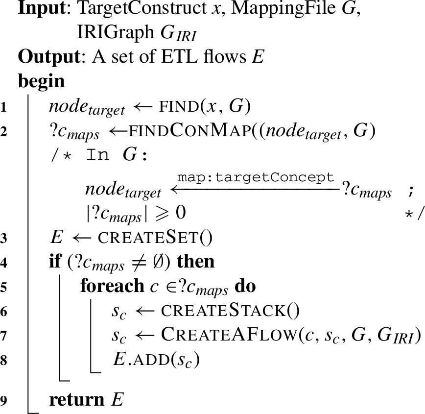
Algorithm 1:
CreateETL
Algorithm 2:
CreateAFlow
Algorithm 3:
Parameterize
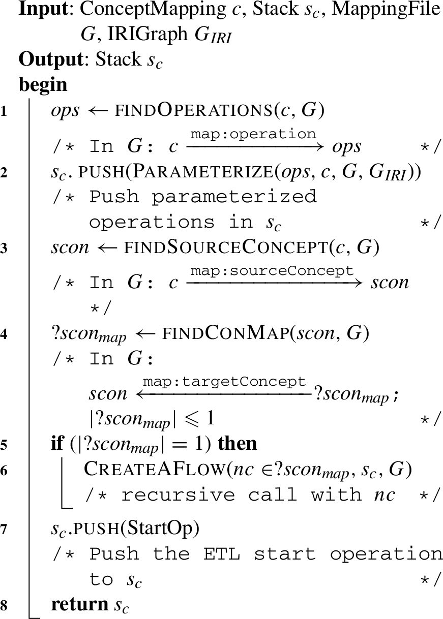
Algorithm 1 shows the steps required to create ETL data flows to populate a target construct (a level, a concept, or a dataset). As inputs, the algorithm takes a target construct x, the mapping file G, and the IRI graph
Algorithm 2 generates an ETL data flow for a concept-mapping c and recursively does so if the current concept-mapping source element is connected to another concept-mapping, until it reaches a source element. Algorithm 2 recursively calls itself and uses a stack to preserve the order of the partial ETL data flows created for each concept-mapping. Eventually, the stack contains the whole ETL data flow between the source and target schema.
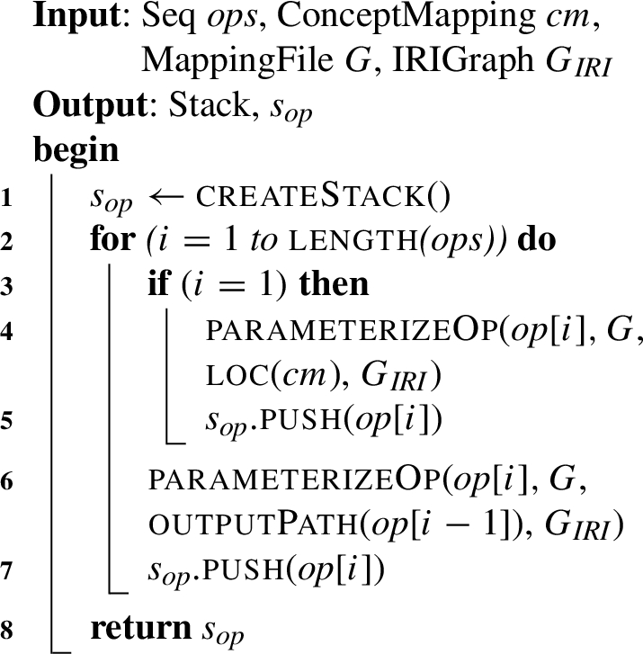
Algorithm 2 works as follows. The sequence of operations in c is pushed to the stack after parameterizing it (lines 1–2). Algorithm 3 parameterizes each operation in the sequence, as described in Section 6 and returns a stack of parameterized operations. As inputs, it takes the operation sequence, the concept-mapping, the mapping file, and the IRI graph. For each operation, it uses the parameterizeOp(
Then, Algorithm 2 traverses to the adjacent concept-mapping of c connected via c’s source concept (line 3–4). After that, the algorithm recursively calls itself for the adjacent concept-mapping (line 6). Note that here, we set a restriction: except for the final target constructs, all the intermediate source and target concepts can be connected to at most one concept-mapping. This constraint is guaranteed when building the metadata in the Definition Layer. Once there are no more intermediate concept-mappings, the algorithm pushes a dummy starting ETL operation (StartOp) (line 7) to the stack and returns it. StartOp can be considered as the root of the ETL data flows that starts the execution process. The stacks generated for each concept-mapping of
7.1.Auto ETL example
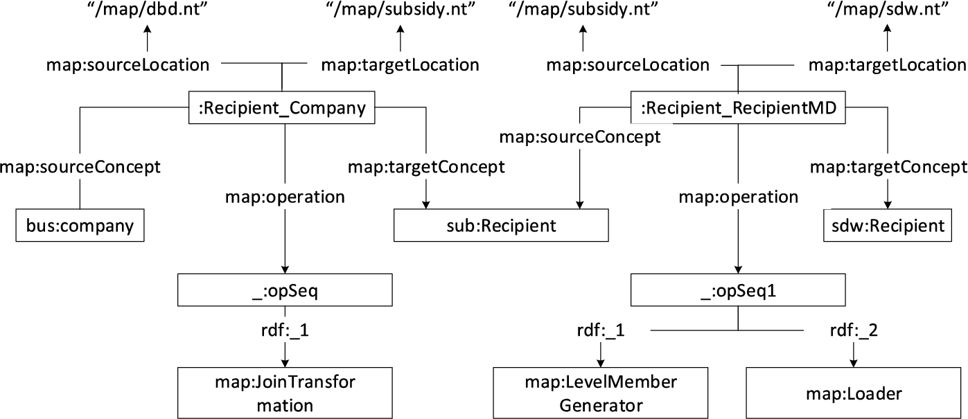
In this section, we show how to populate sdw:Recipient level using CreateETL (Algorithm 1). As input, CreateETL takes the target construct sdw:Recipient, the mapping file Listing 3 and the location of IRI graph “/map/provGraph.nt”. Figure 8 presents a part (necessary to explain this process) of Listing 3 as an RDF graph. As soon as sdw:Recipient is found in the graph, the next task is to find the concept-mappings that are connected to sdw:Recipient through map:targetConcept (line 2). Here, ?cmaps = {:Recipient_RecipientMD}. For :Recipient_RecipientMD, the algorithm creates an empty stack
CreateAFlow retrieves the sequence of operations (line 1) needed to process the concept-mapping, here: ops = (LevelMemberGenerator; Loader) (see Fig. 8). Then, CreateAFlow parameterizes
Then, CreateAFlow finds the source concept of :Recipient_RecipientMD (line 3), which is sub:Recipient; retrieves the concept-mapping :Recipient_Company of sub:Recipient from Listing 3 (line 4); and recursively calls itself for :Recipient_Company (lines 5–6). The operation sequence of :Recipient_Company (line 1) is (JoinTransformation) (see Fig. 8), and the call of Parameterize at line 2 returns the parameterized JoinTransformation(bus:Company, Sub:Reicipient, “/map/dbd.nt”, “/map/subsidy.nt”, comProperty,1515 propertyMappings1616) operation, which is pushed to the stack
8.Evaluation
We created a GUI-based prototype, named SETLCONSTRUCT [17] based on the different high-level constructs described in Sections 5 and 6. We use Jena 3.4.0 to process, store, and query RDF data and Jena TDB as a triplestore. SETLCONSTRUCT is developed in Java 8. Like other traditional tools (e.g., PDI [11]), SETLCONSTRUCT allows developers to create ETL flows by dragging, dropping, and connecting the ETL operations. The system is demonstrated in [17]. On top of SETLCONSTRUCT, we implement the automatic ETL execution flow generation process discussed in Section 7; we call it SETLAUTO. The source code, examples, and developer manual for SETLCONSTRUCT and SETLAUTO are available at https://github.com/bi-setl/SETL.
To evaluate SETLCONSTRUCT and SETLAUTO, we create an MD SDW by integrating the Danish Business Dataset (DBD) [3] and the Subsidy dataset ( https://data.farmsubsidy.org/Old/), described in Section 3. We choose this use case and these datasets for evaluation as there already exists an MD SDW, based on these datasets, that has been programatically created using SETLPROG[44]. Our evaluation focuses on three aspects: 1) productivity, i.e., to what extent SETLCONSTRUCT and SETLAUTO ease the work of a developer when developing an ETL task to process semantic data, 2) development time, the time to develop an ETL process, and 3) performance, the time required to run the process. We run the experiments on a laptop with a 2.10 GHz Intel Core(TM) i7-4600U processor, 8 GB RAM, and Windows 10. On top of that we also present the qualitative evaluation of our approach.
In this evaluation process, we use SETLPROG as our competitive system. We could not directly compare SETLCONSTRUCT and SETLAUTO with traditional ETL tools (e.g., PDI, pygramETL) because they 1) do not support semantic-aware data, 2) are not compatible with the SW technology, and 3) cannot supprot a data warehouse that is semantically defined. On the other hand, we could also not compare them with existing semantic ETL tools (e.g., PoolParty) because they do not support multidimensional semantics at the TBox and ABox level. Therefore, they do not provide any operations for creating RDF data following multidimensional principles. Nevertheless, SETLPROG supports both semantic and non-semantic source integration, and it uses the relational model as a canonical model. In [44], SETLPROG is compared with PDI to some extent. We also present the summary of that comparison in the following sections. We direct readers to [44] for further details.
Table 2
Comparison among the productivity of SETLPROG, SETLCONSTRUCT, and SETLAUTO for the SDW
| Tool ⇒ | SETLPROG | SETLCONSTRUCT | SETLAUTO | ||||||||||
| NOUC | Components of Each Concept | NOUC | Components of Each Concept | ||||||||||
| ETL Task ⇓ | Sub construct | Procedures/Data structures | NUEP | NOTC | Task/Operation | Clicks | Selections | NOTC | Clicks | Selections | NOTC | ||
| TBox with MD Semantics | Cube Structure | Concept(), Property(), BlankNode(), Namespaces(), conceptPropertyBindings(), createOntology() | 1 | 665 | TargetTBoxDefinition | 1 | 9 | 9 | 7 | 1 | 9 | 9 | 7 |
| Cube Dataset | 1 | 67 | 1 | 2 | 2 | 18 | 1 | 2 | 2 | 18 | |||
| Dimension | 2 | 245 | 2 | 3 | 4 | 12 | 2 | 3 | 4 | 12 | |||
| Hierarchy | 7 | 303 | 7 | 4 | 6 | 18 | 7 | 4 | 6 | 18 | |||
| Level | 16 | 219 | 16 | 4 | 5 | 17 | 16 | 4 | 5 | 17 | |||
| Level Attribute | 38 | 228 | 38 | 4 | 3 | 15 | 38 | 4 | 3 | 15 | |||
| Rollup Property | 12 | 83 | 12 | 2 | 1 | 7 | 12 | 2 | 1 | 7 | |||
| Measure Property | 1 | 82 | 1 | 4 | 3 | 25 | 1 | 4 | 3 | 25 | |||
| Hierarchy Step | 12 | 315 | 12 | 6 | 6 | 6 | 12 | 6 | 6 | 6 | |||
| Prefix | 21 | 74 | 21 | 1 | 0 | 48 | 21 | 1 | 0 | 48 | |||
| Subtotal (for the Target TBox) | 1 | 24509 | 101 | 382 | 342 | 1905 | 101 | 382 | 342 | 1905 | |||
| Mapping Generation | Mapping Dataset | N/A | 0 | 0 | SourceToTargetMapping | 5 | 1 | 2 | 6 | 3 | 1 | 2 | 6 |
| Concept-mapping | dict() | 17 | 243 | 23 | 9 | 10 | 0 | 18 | 12 | 10 | 15 | ||
| Property-mapping | N/A | 0 | 0 | 59 | 2 | 2 | 0 | 44 | 2 | 2 | 0 | ||
| Subtotal (for the Mapping File) | 1 | 2052 | 87 | 330 | 358 | 30 | 65 | 253 | 274 | 473 | |||
| Semantic Data Extraction from an RDF Dump File | – | query() | 17 | 40 | GraphExtractor | 17 | 5 | 0 | 30 | 1 | Auto Generation | ||
| Semantic Data Extraction through a SPARQL Endpoint | – | ExtractTriplesFromEndpoint() | 0 | 100 | GraphExtractor | 0 | 5 | 0 | 30 | 0 | Auto Generation | ||
| Cleansing | – | Built-in Petl functions | 15 | 80 | TransformationOnLiteral | 5 | 12 | 1 | 0 | 1 | Auto Generation | ||
| Join | – | Built-in Petl functions | 1 | 112 | JoinTransformation | 1 | 15 | 1 | 0 | 1 | Auto Generation | ||
Table 2
(Continued)
| Tool ⇒ | SETLPROG | SETLCONSTRUCT | SETLAUTO | ||||||||||
| NOUC | Components of Each Concept | NOUC | Components of Each Concept | ||||||||||
| ETL Task ⇓ | Sub construct | Procedures/Data structures | NUEP | NOTC | Task/Operation | Clicks | Selections | NOTC | Clicks | Selections | NOTC | ||
| Level Member Generation | – | createDataTripleToFile(), createDataTripleToTripleStore() | 16 | 75 | LevelMemberGenerator | 16 | 6 | 6 | 0 | 1 | Auto Generation | ||
| Observation Generation | – | createDataTripleToFile(), createDataTripleToTripleStore() | 1 | 75 | ObservationGenerator | 1 | 6 | 6 | 0 | 1 | Auto Generation | ||
| Loading as RDF Dump | – | insertTriplesIntoTDB(), bulkLoadToTDB() | 0 | 113 | Loader | 0 | 1 | 2 | 0 | 0 | Auto Generation | ||
| Loading to a Triplestore | – | insertTriplesIntoTDB(), bulkLoadToTDB() | 17 | 153 | Loader | 17 | 1 | 2 | 0 | 1 | Auto Generation | ||
| Auto ETL Generation | – | – | – | – | CreateETL | 1 | – | – | – | 1 | 21 | 16 | 0 |
| Total (for the Execution Layer Tasks) | 1 | 2807 | 57 | 279 | 142 | 363 | 58 | 21 | 16 | 0 | |||
| Grand Total (for the Whole ETL Process) | 1 | 29358 | 245 | 991 | 826 | 2298 | 224 | 656 | 632 | 2378 | |||
Table 3
Comparison between the ETL processes of SETLPROG and PDI for SDW (Reproduced from [44])
| Tools | SETL | PDI (Kettle) | ||||
| Task | Used tools | Used languages | LOC | Used tools | Used languages | LOC |
| TBox with MD semantics | Built-in SETL | Python | 312 | Protege, SETL | Python | 312 |
| Ontology Parser | Built-in SETL | Python | 2 | User Defined Class | Java | 77 |
| Semantic Data Extraction through SPARQL endpoint | Built-in SETL | Python, SPARQL | 2 | Manually extraction using SPARQL endpoint | SPARQL | NA |
| Semantic Data Extraction from RDF Dump file | Built-in SETL | Python | 2 | NA | NA | NA |
| Reading CSV/Database | Built-in Petl | Python | 2 | Drag & Drop | NA | Number of used Activities: 1 |
| Cleansing | Built-in Petl | Python | 36 | Drag & Drop | NA | Number of used Activities: 19 |
| IRI Generation | Built-in SETL | Python | 2 | User Defined Class | Java | 22 |
| Triple Generation | Built-in SETL | Python | 2 | User Defined Class | Java | 60 |
| External Linking | Built-in SETL | Python | 2 | NA | NA | NA |
| Loading as RDF dump | Built-in SETL | Python | 1 | Drag & Drop | NA | Number of used Activities: 1 |
| Loading to Triple Store | Built-in SETL | Python | 1 | NA | NA | NA |
| Total LOC for the complete ETL process | 401 | 471 LOC + 4 NA + 21 Activities | ||||
8.1.Productivity
SETLPROG requires Python knowledge to maintain and implement an ETL process. On the other hand, using SETLCONSTRUCT and SETLAUTO, a developer can create all the phases of an ETL process by interacting with a GUI. Therefore, they provide a higher level of abstraction to the developer that hides low-level details and requires no programming background. Table 2 summarizes the effort required by the developer to create different ETL tasks using SETLPROG, SETLCONSTRUCT, and SETLAUTO. We measure the developer effort in terms of Number of Typed Characters (NOTC) for SETLPROG and in Number of Used Concepts (NOUC) for SETLCONSTRUCT and SETLAUTO. Here, we define a concept as a GUI component of SETLCONSTRUCT that opens a new window to perform a specific action. A concept is composed of several clicks, selections, and typed characters. For each ETL task, Table 2 lists: 1) its sub construct, required procedures/data structures, number of the task used in the ETL process (NUEP), and NOTC for SETLPROG; 2) the required task/operation, NOUC, and number of clicks, selections, and NOTC (for each concept) for SETLCONSTRUCT and SETLAUTO. Note that NOTC depends on the user input. Here, we generalize it by using same user input for all systems. Therefore, the total NOTC is not the summation of the values of the respective column.
To create a target TBox using SETLPROG, an ETL developer needs to use the following steps: 1) defining the TBox constructs by instantiating the Concept, Property, and BlankNode classes that play a meta modeling role for the constructs and 2) calling conceptPropertyBinding() and createTriples(). Both procedures take the list of all concepts, properties, and blank nodes as parameters. The former one internally connects the constructs to each other, and the latter creates triples for the TBox. To create the TBox of our SDW using SETLPROG, we used 24,509 NOTC. On the other hand, SETLCONSTRUCT and SETLAUTO use the TargetTBoxDefinition interface to create/edit a target TBox. To create the target TBox of our SDW in SETLCONSTRUCT and SETLAUTO, we use 101 concepts that require only 382 clicks, 342 selections, and 1905 NOTC. Therefore, for creating a target TBox, SETLCONSTRUCT and SETLAUTO use 92% fewer NOTC than SETLPROG.
To create source-to-target mappings, SETLPROG uses Python dictionaries where the keys of each dictionary represent source constructs and values are the mapped target TBox constructs, and for creating the ETL process it uses 23 dictionaries, where the biggest dictionary used in the ETL process takes 253 NOTC. In total, SETLPROG uses 2052 NOTC for creating mappings for the whole ETL process. On the contrary, SETLCONSTRUCT and SETLAUTO use a GUI. In total, SETLCONSTRUCT uses 87 concepts composed of 330 clicks, 358 selections, and 30 NOTC. Since SETLAUTO internally creates the intermediate mappings, there is no need to create separate mapping datasets and concept-mappings for intermediate results. Thus, SETLAUTO uses only 65 concepts requiring 253 clicks, 274 selections, and 473 NOTC. Therefore, SETLCONSTRUCT reduces NOTC of SETLPROG by 98%. Although SETLAUTO uses 22 less concepts than SETLCONSTRUCT, SETLCONSTRUCT reduces NOTC of SETLAUTO by 93%. This is because, in SETLAUTO, we write the data extraction queries in the concept-mappings where in SETLCONSTRUCT we set the data extraction queries in the ETL operation level.
To extract data from either an RDF local file or an SPARQL endpoint, SETLPROG uses the query() procedure and the ExtractTriplesFromEndpoint() class. On the other hand, SETLCONSTRUCT uses the GraphExtractor operation. It uses 1 concept composed of 5 clicks and 20 NOTC for the local file and 1 concept with 5 clicks and 30 NOTC for the endpoint. SETLPROG uses different functions/procedures from the Petl Python library (integrated with SETLPROG) based on the cleansing requirements. In SETLCONSTRUCT, all data cleansing related tasks on data sources are done using TransformationOnLiteral (single source) and JoinTransformation (for multi-source). TransformationOnLiteral requires 12 clicks and 1 selection, and JoinTransformation takes 15 clicks and 1 selection.
To create a level member and observation, SETLPROG uses createDataTripleToFile() and takes 125 NOTC. The procedure takes all the classes, properties, and blank nodes of a target TBox as input; therefore, the given TBox should be parsed for being used in the procedure. On the other hand, SETLCONSTRUCT uses the LevelMemberGenerator and ObservationGenerator operations, and each operation requires 1 concept, which takes 6 clicks and 6 selections. SETLPROG provides procedures for either bulk or trickle loading to a file or an endpoint. Both procedures take 113 and 153 NOTC, respectively. For loading RDF triples either to a file or a triple store, SETLCONSTRUCT uses the Loader operation, which needs 2 clicks and 2 selections. Therefore, SETLCONSTRUCT reduces NOTC for all transformation and loading tasks by 100%.
SETLAUTO requires only a target TBox and a mapping file to generate ETL data flows through the CreateETL interface, which takes only 1 concept composed of 21 clicks and 16 selections. Therefore, other ETL Layer tasks are automatically accomplished internally. In summary, SETLCONSTRUCT uses 92% fewer NOTC than SETLPROG, and SETLAUTO further reduces NOUC by another 25%.
8.1.1.Comparison between SETLPROG and PDI
PDI is a non-semantic data integration tool that contains a rich set of data integration functionality to create an ETL solution. It does not support any functionality for semantic integration. In [44], we used PDI in combination with other tools and manual tasks to create a version of an SDW. The comparison between the ETL processes of SETLPROG and PDI to create this SDW are shown in Table 3. Here, we outline the developer efforts in terms of used tools, languages, and Lines of Codes (LOC). As mentioned earlier, SETLPROG provides built-in classes to annotate MD constructs with a TBox. PDI does not support defining a TBox. To create the SDW using PDI, we use the TBox created by SETLPROG. SETLPROG provides built-in classes to parse a given TBox and users can use different methods to parse the TBox based on their requirements. In PDI, we implement a Java class to parse the TBox created by SETLPROG which takes an RDF file containing the definition of a TBox as input and outputs the list of concepts and properties contained in the TBox. PDI is a non-semantic data integration tool, thus, it does not support processing semantic data. We manually extract data from SPARQL endpoints and materialize them in a relational database for further processing. PDI provides activities (drag & drop functionality) to pre-process database and CSV files. On the other hand, SETLPROG provides methods to extract semantic data either from a SPARQL endpoint or an RDF dump file batch-wise. In SETLPROG, users can create an IRI by simply passing arguments to the createIRI () method. PDI does not include any functionality to create IRIs for resources. We define a Java class of 23 lines to enable the creation of IRIs for resources. SETLPROG provides the createTriple() method to generate triples from the source data based on the MD semantics of the target TBox; users can just call it by passing required arguments. In PDI, we develop a Java class of 60 lines to create the triples for the sources. PDI does not support to load data directly to a triple store which can easily be done by SETLPROG. Finally, we could not run the ETL process of PDI automatically (i.e., in a single pass) to create the version of a SDW. We instead made it with a significant number of user interactions. In total, SETLPROG takes 401 Lines of Code (LOC) to run the ETL, where PDI takes
Therefore, we can conclude that SETLPROG uses 14.9% less LOC than PDI, SETLCONSTRUCT uses 92% fewer NOTC than SETLPROG, and SETLAUTO further reduces NOUC by another 25%. Combining these results, we see that SETLCONSTRUCT and SETLAUTO have significantly better productivity than PDI for building an SDW.
8.2.Development time
We compare the time used by SETLPROG, SETLCONSTRUCT, and SETLAUTO to build the ETL processes for our use case SDW. As the three tools were developed within the same project scope and we master them, the first author conducted this test. We chose the running use case used in this paper and created a solution in each of the three tools and measured the development time. We used each tool twice to simulate the improvement we may obtain when we are knowledgeable about a given project. The first time it takes more time to analyze, think, and create the ETL process, and in the latter, we reduce the interaction time spent on analysis, typing, and clicking. Table 4 shows the development time (in minutes) for main integration tasks used by the different systems to create the ETL processes.
Table 4
ETL development time (in minutes) required for SETLPROG, SETLCONSTRUCT, and SETLAUTO
| Tool | Iteration number | Target TBox definition | Mapping generation | ETL design | Total |
| SETLPROG | 1 | 186 | 51 | 85 | 322 |
| SETLPROG | 2 | 146 | 30 | 65 | 241 |
| SETLCONSTRUCT | 1 | 97 | 46 | 35 | 178 |
| SETLCONSTRUCT | 2 | 58 | 36 | 30 | 124 |
| SETLAUTO | 1 | 97 | 40 | 2 | 139 |
| SETLAUTO | 2 | 58 | 34 | 2 | 94 |
Fig. 9.
The segment of the main method to populate the sdw:SubsidyMD dataset and the sdw:Recipient using SETLPROG.
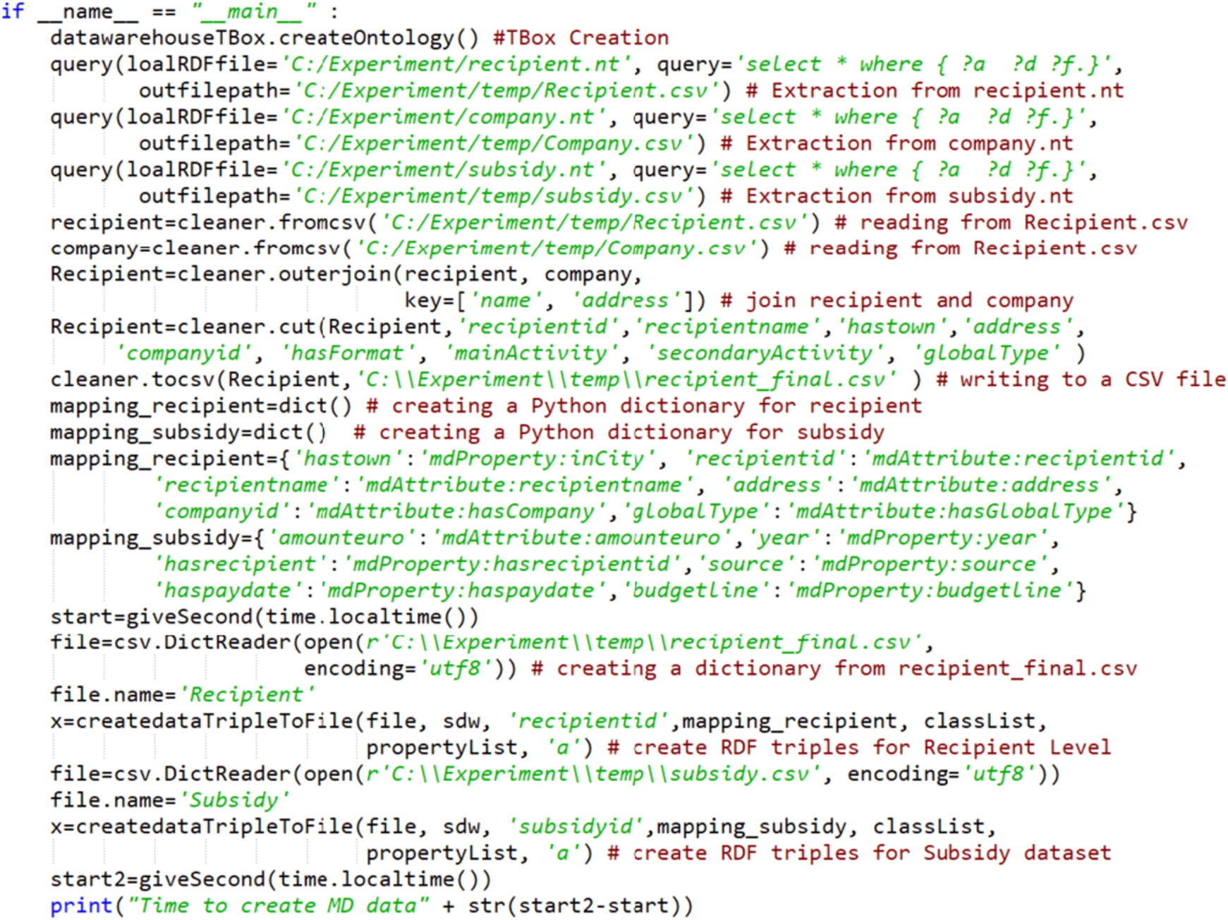
Fig. 10.
The ETL flows to populate the sdw:SubsidyMD dataset and the sdw:Recipient level using SETLCONSTRUCT.
SETLPROG took twice as long as SETLCONSTRUCT and SETLAUTO to develop a target TBox. In SETLPROG, to create a target TBox construct, for example a level l, we need to instantiate the Concept() concept for l and then add its different property values by calling different methods of Concept(). SETLCONSTRUCT and SETLAUTO create l by typing the input or selecting from the suggested items. Thus, SETLCONSTRUCT and SETLAUTO also reduce the risk of making mistakes in an error-prone task, such as creating an ETL. In SETLPROG, we typed all the source and target properties to create a mapping dictionary for each source and target concept pair. However, to create mappings, SETLCONSTRUCT and SETLAUTO select different constructs from a source as well as a target TBox and only need to type when there are expressions and/or filter conditions of queries. Moreover, SETLAUTO took less time than SETLCONSTRUCT in mapping generation because we did not need to create mappings for intermediate results.
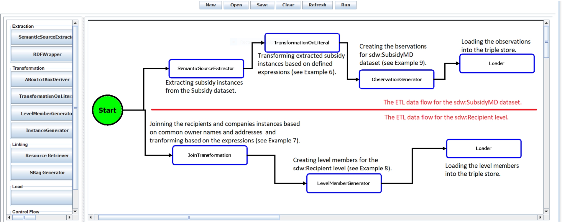
To create ETL data flows using SETLPROG, we had to write scripts for cleansing, extracting, transforming, and loading. SETLCONSTRUCT creates ETL flows using drag-and-drop options. Note that the mappings in SETLCONSTRUCT and SETLAUTO use expressions to deal with cleansing and transforming related tasks; however, in SETLPROG we cleansed and transformed the data in the ETL design phase. Hence, SETLPROG took more time in designing ETL compared to SETLCONSTRUCT. On the other hand, SETLAUTO creates the ETL data flows automatically from a given mapping file and the target TBox. Therefore, SETLAUTO took only two minutes to create the flows. In short, SETLPROG is a programmatic environment, while SETLCONSTRUCT and SETLAUTO are drag and drop tools. We exemplify this fact by means of Figs 9 and 10, which showcase the creation of the ETL data flows for the sdw:SubsidyMD dataset and the sdw:Recipient level. To make it more readable and understandable, we add comments at the end of the lines of Fig. 9 and in each operation of Fig. 10. In summary, using SETLCONSTRUCT, the development time is cut in almost half (41% less development time than SETLPROG); and using SETLAUTO, it is cut by another 27%.
Table 5
ETL execution time (in minutes) required for each sub-phase of the ETL processes created using SETLPROG and SETLCONSTRUCT
| Performance metrics | Systems | Extraction and traditional transformation | Semantic transformation | Loading | Total processing time |
| Processing time (in minutes) | SETLPROG | 33 | 17.86 | 21 | 71.86 |
| SETLCONSTRUCT | 43.05 | 39.42 | 19 | 101.47 | |
| Input size | SETLPROG | 6.2 GB (Jena TDB) + 6.1 GB (N-Triples) | 496 MB (CSV) | 4.1 GB (N-Triples) | |
| SETLCONSTRUCT | 6.2 GB (Jena TDB) + 6.1 GB (N-Triples) | 6.270 GB (N-Triples) | 4.1 GB (N-Triples) | ||
| Output size | SETLPROG | 490 MB (CSV) | 4.1 GB (N-Tripels) | 3.7 GB (Jena TDB) | |
| SETLCONSTRUCT | 6.270 GB (N-Triples) | 4.1 GB (N-Triples) | 3.7 GB (Jena TDB) |
8.3.Performance
Since the ETL processes of SETLCONSTRUCT and SETLAUTO are the same and only differ in the developer effort needed to create them, this section only compares the performance of SETLPROG and SETLCONSTRUCT. We do so by analyzing the time required to create the use case SDW by executing the respective ETL processes. To evaluate the performance of similar types of operations, we divide an ETL process into three sub-phases: extraction and traditional transformation, semantic transformation, as well as loading and discuss the time to complete each.
Table 5 shows the processing time (in minutes), input and output size of each sub-phase of the ETL processes created by SETLPROG and SETLCONSTRUCT. The input and output formats of each sub-phase are shown in parentheses. The extraction and traditional transformation sub-phases in both systems took more time than the other sub-phases. This is because they include time for 1) extracting data from large RDF files, 2) cleansing and filtering the noisy data from the DBD and Subsidy datasets, and 3) joining the DBD and Subsidy datasets. SETLCONSTRUCT took more time than SETLPROG because its TransformationOnLiteral and JoinTransformation operations use SPARQL queries to process the input file whereas SETLPROG uses the methods from the Petl Python library to cleanse the data extracted from the sources.
SETLCONSTRUCT took more time during the semantic transformation than SETLPROG because SETLCONSTRUCT introduces two improvements over SETLPROG: 1) To guarantee the uniqueness of an IRI, before creating an IRI for a target TBox construct (e.g., a level member, an instance, an observation, or the value of an object or roll-up property), the operations of SETLCONSTRUCT search the IRI provenance graph to check the availability of an existing IRI for that TBox construct. 2) As input, the operations of SETLCONSTRUCT take RDF (N-triples) files that are larger in size than the CSV files (see Table 5), used by SETLPROG as input format. To ensure our claims, we run an experiment for measuring the performance of the semantic transformation procedures of SETLPROG and the operations of SETLCONSTRUCT by excluding the additional two features introduced in SETLCONSTRUCT operations (i.e., a SETLCONSTRUCT operation does not lookup the IRI provenance graph before creating IRIs and takes a CSV input). Figure 11 shows the processing time taken by SETLCONSTRUCT operations and SETLPROG procedures to create level members and observations with increasing input size. In the figure, LG and OG represent level member generator and observation generator operations (in case of SETLCONSTRUCT) or procedures (in case of SETLPROG).
Fig. 11.
Comparison of SETLCONSTRUCT and SETLPROG for semantic transformation. Here, LG and OG stand for LevelMemberGenerator and ObservationGenerator.
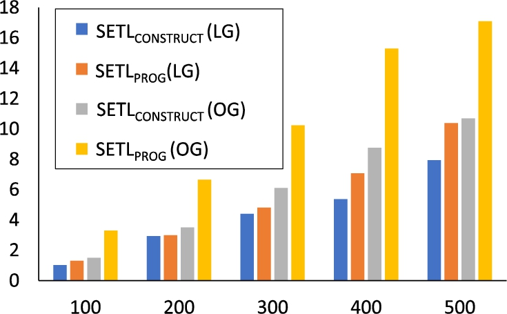
Fig. 12.
Scalability of LevelMemberGenerator and ObservationGenerator.
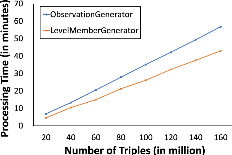
In summary, to process an input CSV file with 500 MB in size, SETLCONSTRUCT takes 37.4% less time than SETLPROG to create observations and 23.4% less time than SETLPROG to create level members. The figure also shows that the processing time difference between the corresponding SETLCONSTRUCT operation and the SETLPROG procedure increases with the size of the input. In order to guarantee scalability when using the Jena library, a SETLCONSTRUCT operation takes the (large) RDF input in the N-triple format, divides the file into several smaller chunks, and processes each chunk separately. Figure 12 shows the processing time taken by LevelMemberGenerator and ObservationGenerator operations with the increasing number of triples. We show the scalability of the LevelMemberGenerator and ObservationGenerator because they create data with MD semantics. The figure shows that the processing time of both operations increase linearly with the increase in the number of triples, which ensures that both operations are scalable. SETLCONSTRUCT takes less time in loading than SETLPROG because SETLPROG uses the Jena TDB loader command to load the data while SETLCONSTRUCT programmatically load the data using the Jena API’s method.
In summary, SETLPROG and SETLCONSTRUCT have similar performance (29% difference in total processing time). SETLCONSTRUCT ensures the uniqueness of IRI creation and uses RDF as a canonical model, which makes it more general and powerful than SETLPROG.
Besides the differences of the performances already explained in Table 5, SETLCONSTRUCT also includes an operation to update the members of the SDW levels, which is not included in SETLPROG. Since the ETL process for our use case SDW did not include that operation, we scrutinize the performance of this specific operation of SETLCONSTRUCT in the following.
Fig. 13.
Performance of UpdateLevel based on processing time and target ABox size with the changing of the sdw:Recipient and sdw:City members.
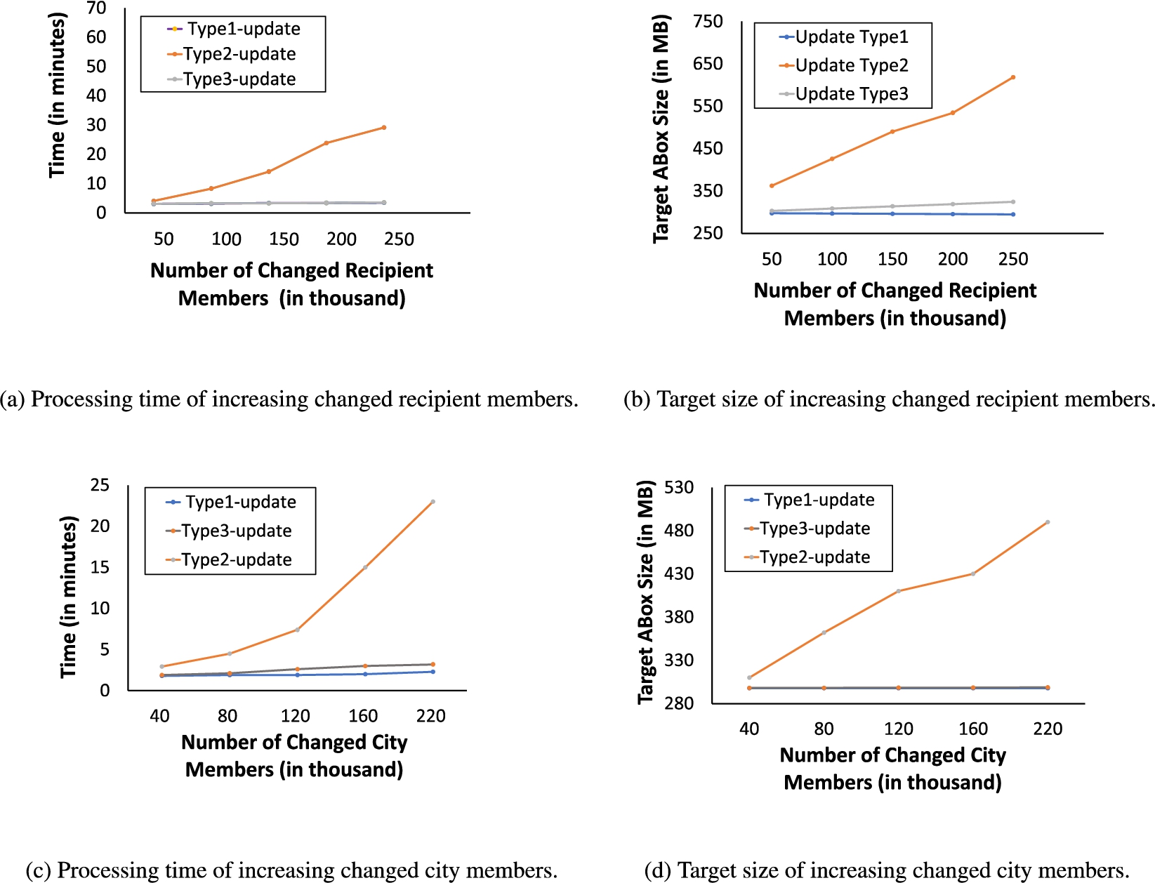
Performance analysis of UpdateLevel operation Figure 13 shows the performance of the UpdateLevel operation. To evaluate this operation, we consider two levels: mdProperty:Recipient and mdProperty:City. We consider these two levels because mdProperty:Recipient is the largest level (in terms of size) in our use case, and mdProperty:City is the immediate upper level of mdProperty:Recipient in the mdStructure:Address hierarchy of the dimension mdProperty:Beneficiary. Therefore, we can record how the changes in cities propagate to recipients, especially in Type2-update. The sdw:Recipient level is the lowest granularity level in the mdStructure:Address hierarchy; therefore, changes in a recipient (i.e., a member of sdw:Recipient) only affect that recipient. Figure 13a shows the processing time with the increasing number of recipients. As a Type2-update creates a new version for each changed level member, it takes more time than a Type1-update and a Type3-update. A Type3-update takes more time than a Type1-update because it keeps the record of old property values besides the current ones. Figure 13b shows how the size of the target ABox increases with the increasing number of recipients. The target ABox size increases linearly with the increasing number of recipients (see Fig. 13b) for Type2-update and Type-3 updates because they keep additional information. However, the target ABox size decreases with the increasing number of recipients for Type1-updates; this is because the current property-values are smaller than the older ones in size.
Figure 13c shows the processing time when increasing the number of updated cities. Since sdw:City is the immediate upper level of sdw:Recipient in the mdStructure:address hierarchy, to reflect a changed city in the target ABox, a Type2-update creates new versions for itself as well as for the recipients living in that city. Therefore, a Type2-update takes more processing time in comparison to a Type1-update and a Type-3 update. Figure 13d shows the target ABox size with the increasing number of cities. The figure shows that the target ABox size for Type2-updates increases slowly within the range from 120 to 160 (X-axis), and it indicates that the changed cities within this range contain fewer recipients than the cities in other ranges.
8.3.1.Comparison between SETLPROG and PDI in processing sdw:Subsidy
In [44], we compare the performance of SETLPROG with a non-semantic data integration tool, PDI. We populate the SDW for sdw:Subsidy concept using PDI. To run the process PDI takes 1903 s. On other hand, SETL takes only 1644 s. Thus, SETL is 259 s (13.5%) faster than PDI. PDI is much slower because almost everything MD-related must be embedded as UDFs or equivalent elements.
In overall, we conclude that SETLPROG is better in performance compared to PDI and SETLCONSTRUCT. However, SETLCONSTRUCT is a more correct and scalable framework. On top of that, SETLCONSTRUCT supports SDWs update.
8.4.Qualitative evaluation
To evaluate our proposed high-level ETL qualitatively, we selected and interviewed two experts with expertise across traditional ETL and semantic integration. We find that two experts are sufficient, because both of them have 10+ years research experiences in ETL and are the architects of popular open-source ETL tools (pygramETL [60] and QUARRY [33]). In this section, we present a high-level summary of the expert interviews. We follow the procedure described in [10,42] to structure the questionnaire and the answers of the experts. The two experts participated in the interviews via email. Interviews included nine semi-structured questions1717 aimed at gathering expert opinions on the significance of the proposed two-layered RDF-based semantic data integration paradigm, completeness and soundness of the proposed set of ETL operations, and further possibilities of the proposed approach. Table 6 shows the questions, their categories, and the responses as well as justifications of both experts. A response is rated from 1 to 5 (1 – strongly disagree, 2 – disagree, 3 – neutral, 4 – agree, and 5 -strongly agree). Q4, Q7, Q8, and Q9 contain free-text answers only.
Table 6
Summary of the expert interviews
| Category | No. | Questions | Expert 1 | Expert 2 | ||
| Response | Justification | Response | Justification | |||
| Significance of the proposed paradigm | Q1 | Is the two-layered paradigm followed by SETLCONSTRUCTmore convenient than the traditional approach? | 5 | Separation of Concerns | 4 | The intervention of more technical users is required |
| Q2 | Are the metadata artifacts from Definition Layer sufficient to deal with real-case problems? | 4 | Extensibility by the user would be useful | 3 | Complete for the ETL specific to semantic data and multidimensional analysis | |
| Q3 | Do you consider SETLCONSTRUCT’s target-driven approach to build semantic data warehouses appropriate? | 4 | 5 | |||
| Q4 | Do you consider \scon\is a valuable and notable contribution compared to traditional ETL tools and semantic-oriented ETL tools? | Yes | Yes | |||
| Soundness and completeness | Q5 | Is the set of ETL operations proposed sound? | 5 | Okay | 3 | The ETL operations seem to be correct |
| Q6 | Are the proposed operations complete? | 5 | Sufficient | 5 | ||
| Q7 | Do you miss anything (else) in scon current set of core ETL operations | UDFs would be useful | Row normalizer/denormalizer | |||
| Further possibilities | Q8 | Do you consider automation of the mapping file is feasible? | Semi-automation is feasible | Not easy to express more complex, black box operations | ||
| Q9 | Do you think our approach fits in the context of Big Data and Data Lakes (and how)? | Yes | Limited to support complex data transformations in the Big Data context | |||
On the significance of the proposed paradigm category, both experts provide positive responses to all questions. Their only suggestion is to allow technical users to extend the metadata artifacts because ETL tool palettes can typically be much more complex. We use RDF as the canonical model in our paradigm, and it allows users to extend metadata artifacts based on their business requirements. Both experts think that our proposed ETL operations are sound and complete considering that the ETL is specific to semantic data and multidimensional analysis. However, one of the suggestions is to make the set of ETL operations open and to introduce user-defined functions (UDFs) so that users can write their own functions if there is a requirement for additional transformations (e.g., row normalizer/denormalizer, language conversion). In our future work, we will introduce UDFs in the set of ETL operations. Both experts do not support complete automation of the mapping file considering the complex nature of ETL scenarios. However, they think that semi-automation is feasible. Expert 1 thinks that we can apply this two-layered RDF-based data integration approach in the context of Big data and Data Lakes. However, Expert 2 thinks that there is a need to support more complex data transformations.
In summary, both experts acknowledge the contribution of our work and think that the set of ETL operations is complete and sound to annotate a knowledge base with multidimensional semantics. However, to fit this approach in the context of Big Data and data lakes, there is a need to include UDFs to support more complex transformations.
9.Related work
Nowadays, combining SW and BI technologies is an emerging research topic as it opens interesting research opportunities. As a DW deals with both internal and (increasingly) external data presented in heterogeneous formats, especially in the RDF format, semantic issues should be considered in the integration process [1]. Furthermore, the popularity of SW data gives rise to new requirements for BI tools to enable OLAP-style analysis over this type of data [32]. Therefore, the existing research related to semantic ETL is divided into two lines: 1) on the one hand, the use of SW technologies to physically integrate heterogeneous sources and 2) on the other hand, enabling OLAP analysis over SW data.
One prominent example following the first research line is [58], which presents an ontology-based approach to enable the construction of ETL flows. At first, the schema of both the sources and the DW are defined by a common graph-based model, named the datastore graph. Then, the semantics of the datastore graphs of the data sources and the DW are described by generating an (OWL-based) application ontology, and the mappings between the sources and the target are established through that ontology. In this way this approach addresses heterogeneity issues among the source and target schemata and finally demonstrates how the use of an ontology enables a high degree of automation from the source to the target attributes, along with the appropriate ETL transformations. Nonetheless, computationally complex ETL operations like slowly changing dimensions and the annotation of the application ontology with MD semantics are not addressed in this work. Therefore, OLAP queries cannot be applied on the generated DW.
Another piece of existing work [6] aligned to this line of research proposes a methodology describing some important steps required to make an SDW, which enables to integrate data from semantic databases. This approach also misses the annotation of the SDW with MD semantics. [59] has proposed an approach to support data integration tasks in two steps: 1) constructing ontologies from XML and relational sources and 2) integrating the derived ontologies by means of existing ontology alignment and merging techniques. However, ontology alignment techniques are complex and error-prone. [5] presents a semantic ETL framework at the conceptual level. This approach utilizes the SW technologies to facilitate the integration process and discusses the use of different available tools to perform different steps of the ETL process. [3] presents a method to spatially integrate a Danish Agricultural dataset and a Danish Business dataset using an ontology. The approach uses SQL views and other manual processes to cleanse the data and Virtuoso for creating and storing integrated RDF data. [38] presents UnifiedViews, an open-source ETL framework that supports management of RDF data. Based on the SPARQL queries, they define four types of Data Processing Units (DPUs): Extractor, Transformer, Loader, and Quality Assessor. However, the DPUs do not support to generate MD RDF data.
In the second line of research, a prominent paper is [47], which outlines a semi-automatic method for incorporating SW data into a traditional MD data management system for OLAP analysis. The proposed method allows an analyst to accomplish the following tasks: 1) designing the MD schema from the TBox of an RDF dataset, 2) extracting the facts from the ABox of the dataset and populating the MD fact table, and 3) producing the dimension hierarchies from instances of the fact table and the TBox to enable MDX queries over the generated DW. However, the generated DW no longer preserves the SW data principles defined in [27]; thus, OLAP analysis directly over SW data is yet to be addressed. To address this issue, [13] introduces the notion of a lens, called the analytical schema, over an RDF dataset. An analytical schema is a graph of classes and properties, where each node of the schema presents a set of facts that can be analyzed by traversing the reachable nodes. [28] presents a self-service OLAP endpoint for an RDF dataset. This approach first superimposes an MD schema over the RDF dataset. Then, a semantic analysis graph is generated on top of that MD schema, where each node of the graph represents an analysis situation corresponding to an MD query, and an edge indicates a set of OLAP operations.
Both [13] and [28] require either a lens or a semantic analysis graph to define MD views over an RDF dataset. Since most published SW data contains facts and figures, W3C recommends the Data Cube (QB) [15] vocabulary to standardize the publication of SW data with MD semantics. Although QB is appropriate to publish statistical data and several publishers (e.g., [51]) have already used the vocabulary for publishing statistical datasets, it has limitations to define MD semantics properly. The QB4OLAP [20] vocabulary enriches QB to support MD semantics by providing constructs to define 1) a cube structure in terms of different level of dimensions, measures, and attaching aggregate functions with measures and 2) a dimension structure in terms of levels, level attributes, relationships, the cardinality of relationships among the levels, and hierarchies of the dimension. Therefore, MD data can be published either by enriching data already published using QB with dimension levels, level members, dimension hierarchies, and the association of aggregate functions to measures without affecting the existing observations [62] or using QB4OLAP from scratch [22,29,44].
In [36], the authors present an approach to enable OLAP operations on a single data cube published using the QB vocabulary and shown the applicability of their OLAP-to-SPARQL mapping in answering business questions in the financial domain. However, their OLAP-to-SPARQL mapping may not result in the most efficient SPARQL query and requires additional efforts and a longer time to get the results as they consider that the cube is queried on demand and the DW is not materialized. While some approaches have proposed techniques to optimize execution of OLAP-style SPARQL queries in a federated setting [30], others have considered view materialization [21,31]. The authors in [62] present a semi-automatic method to enrich the QB dataset with QB4OLAP terms. However, there is no guideline for an ETL process to populate a DW annotated with QB4OLAP terms.
After analyzing the two research lines, we can draw some conclusions. Although each approach described above addresses one or more aspects of a semantic ETL framework, there is no single platform that supports them all (target definition, source-to-target mappings generation, ETL generations, MD target population, and evolution). To solve this problem, we have proposed a Python-based programmable semantic ETL (SETLPROG) framework [44] that provides a number of powerful modules, classes, and methods for performing the tasks mentioned above. It facilitates developers by providing a higher abstraction level that lowers the entry barriers. We have experimentally shown that SETLPROG performs better in terms of programmer productivity, knowledge base quality, and performance, compared to other existing solutions. However, to use it, developers need a programming background. Although SETLPROG enables to create an ETL flow and provides methods by combining several tasks, there is a lack of a well-defined set of basic semantic ETL constructs that allow users more control in creating their ETL process. Moreover, how to update an SDW to synchronize it with the changes taking place in the sources is not discussed. Further, in a data lake/big data environment, the data may come from heterogeneous formats, and the use of the relational model as the canonical model may generate an overhead. Transforming JSON or XML data to relational data to finally generate RDF can be avoided by using RDF as the canonical model instead. To this end, several works have discussed the appropriateness of knowledge graphs for data integration purposes and specifically, as a canonical data model [14,54,55]. An additional benefit of using RDF as a canonical model is that it allows adding semantics without being compliant to a fixed schema. The present paper presents the improvements introduced on top of SETLPROG to remedy its main drawbacks discussed above. As there are available RDF Wrappers (e.g., [18,57]) to convert another format to RDF, in this paper, we focus on only semantic data and propose an RDF-based two-layered (Definition Layer and Execution Layer) integration process. We also propose a set of high-level ETL constructs (tasks/operations) for each layer, with the aim of overcoming the drawbacks identified above for SETLPROG. We also provide an operation to update an SDW based on the changes in source data. On top of that, we characterize the ETL flow in the Definition Layer by means of creating an RDF based source-to-target mapping file, which allows to automate the ETL execution flows.
10.Conclusion and future work
In this paper, we proposed a framework of a set of high-level ETL constructs to integrate semantic data sources. The overall integration process uses the RDF model as canonical model and is divided into the Definition and Execution Layer. In the Definition Layer, ETL developers create the metadata (target and source TBoxes, and source-to-target mappings). We propose a set of high-level ETL operations for semantic data that can be used to create ETL data flows in the Execution Layer. As we characterize the transformations in the Definition Layer in terms of source-to-target mappings at the schema level, we are able to propose an automatic algorithm to generate ETL data flows in the Execution Layer. We developed an end-to-end prototype SETLCONSTRUCT based on the high-level constructs proposed in this paper. We also extended it to enable automatic ETL execution flows generation (and named it SETLAUTO). The experiment shows that 1) SETLCONSTRUCT uses 92% fewer NOTC than SETLPROG, and SETLAUTO further reduces NOUC by another 25%; 2) usingSETLCONSTRUCT, the development time is almost cut in half compared to SETLPROG, and is cut by another 27% using SETLAUTO; 3) SETLCONSTRUCT is scalable and has similar performance compared to SETLPROG.
SETLCONSTRUCT allows users to create source-to-target mappings manually. However, an extension of this work is to create the mappings (semi-)automatically. Although this kind of ETL mappings is different from traditional ontology schema matching techniques, we can explore those techniques to establish the relationships among the concepts across the source and target ontologies. Taking the output of this schema matching approach as a suggestion, the expert can enrich the mappings according to the business requirements [41]. As the correctness of an ontology schema matching technique depends on the semantic-richness of the given ontologies, besides the extensional knowledge given in the ABox, we need to take other external standard ontologies into account in the process of the TBoxExtraction operation.
The source-to-target mappings act as a mediator to generate data according to the semantics encoded in the target. Therefore, we plan to extend our framework from purely physical to also virtual data integration where instead of materializing all source data in the DW, ETL processes will run on demand. When considering virtual data integration, it is important to develop query optimization techniques for OLAP queries on virtual semantic DWs, similar to the ones developed for virtual integration of data cubes and XML data [48,49,63]. Another interesting work will be to apply this layer-based integration process in a Big Data and Data Lake environment. The metadata produced in the Definition Layer can be used as basis to develop advanced catalog features for Data Lakes. We will also introduce user-defined functions (UDFs) and other relevant ETL operations to make the approach fit in the Big Data context, as suggested by the two interviewed experts. Furthermore, we plan to investigate how to integrate provenance information into the process [2]. Another aspect of future work is the support of spatial data [23,24].
Notes
4 Here, we use the terms “target” and “MD SDW” interchangeably.
5 An operation has a side effect if it modifies some state variable value(s) outside its local environment (https://en.wikipedia.org/wiki/Side_effect_(computer_science)).
6 To make it easily distinguishable, here, we use comma instead of space to separate the components of a triple pattern and an RDF triple.
7 We present the examples in Turtle format for reducing the space and better understanding. In practice, our system prefers N-Triples format to support scalability.
8 A level is termed as a level property in QB4OLAP, therefore, throughout this paper, we use both the term “level” and “level property” interchangeably.
9 A rule can be either a source property, an expression or incremental, as described in Section 5.
10 The IRI graph is an RDF graph that keeps a triple for each resource in the SDW with their corresponding source IRI.
12 Here, some functions used in the algorithms are characterized by a pattern over G, shown at its side as comments in the corresponding algorithm.
13 Here, lines 95–112 in Listing 3.
14 (..) indicates that the operation is parameterized.
15 lines 32, 36–39 in Listing 3.
16 Lines 76–93 in Listing 3.
18 We follow the same syntax and semantics used in [50] for a query pattern.
19 To make it easily distinguishable, here we use comma to separate the components of a triple pattern and an RDF triple.
20 If the source construct is either a QB level property or dataset, then rdf:type is replaced by either qb4o:memberOf or qb4o:dataset.
21 The term target here does not mean target schema but in the sense it is defined in concept-mappings. Source and target both can be either source concepts or intermediate concepts (from an intermediate result).
Acknowledgements
This research is partially funded by the European Commission through the Erasmus Mundus Joint Doctorate Information Technologies for Business Intelligence (EM IT4BI-DC), the Poul Due Jensen Foundation, and the Danish Council for Independent Research (DFF) under grant agreement no. DFF-8048-00051B.
Appendices
Appendix
A.1.Semantics of the Execution Layer operations
In this section, we provide the detailed semantics of the ETL operations described in Section 6. The operations depend on some auxiliary functions. Here, we first present the semantics of the auxiliary functions and then the semantics of the operations. We present each function and operation in terms of input Parameters and semantics. To distinguish the auxiliary functions from the operations, we use small capital letters to write an auxiliary function name, while an operation name is written in italics.
A.1.1.Auxiliary functions
executeQuery(Q, G,
Input Parameters: Let I, B, L, and V be the sets of IRIs, blank nodes, literals, and query variables. We denote the set of RDF terms
1. An RDF triple pattern
2. If
3. If Q is a query pattern and
Semantics: For the query pattern Q, let μ be a partial function that maps
1. If the query pattern Q is a triple pattern
2. If Q is
3. If Q is
 .
.4. If Q is
5. If
getPropertiesFromExpressions(sTBox, exps) An expression is a combination of one or more properties, operators, and SPARQL functions defined in [25]. This function returns a subset of properties of a source TBox that are used in the given expressions.
Input Parameters: sTBox is a TBox and exps is a set of expressions.
Semantics: For each
This function returns a set of properties.
validateExpressions(
Input Parameters:
Semantics: If
If
mappedSourceInstances(sc, sTBox, sABox, propertyMappings) This function returns a dictionary describing the instances of a source concept.
Input Parameters:
Semantics: At first, this function retrieves instances of
Here, mappedExpressions(sc, propertyMappings) returns the set of source properties/expressions (defined by map:source4TargetPropertyValue) used in propertyMappings. The dictionary((?i, ?p, ?v)) function first groups the input tuples by ?i and then for each instance
generateIRI(sIRI, value, tType, tTBox, iriGraph) Every resource in an SDW is uniquely identified by an IRI defined under the namespace of the SDW. This function creates an equivalent target IRI for a source resource. Additionally, it keeps that information in the IRI graph.
Input Parameters:
Semantics: Equation (3) formulates how to create the IRI. First, the function checks whether there is an equivalent IRI for
This function returns an IRI.
tuplesToTriples(T, tc, Q, propertyMappings, (i,
Input Parameters: T is a set of tuples (1st normal form tabular format),
Semantics: Equation (4) shows the semantics of this function. Each tuple of T represents an instance-to-be of the target construct
This function returns a set of RDF triples.
A.1.2.Execution Layer operations
This section gives the semantics of each operation category-wise.
Extraction Operations
GraphExtractor(Q, G, outputPattern, tABox) This operation is functionally equivalent to SPARQL CONSTRUCT queries to extract data from sources.
Input Parameters: Q is a query pattern as defined in ExecuteQuery(). G is an RDF graph over which Q is evaluated. The parameter
Semantics: This operation generates the output in two steps: 1) First, Q is matched against G to obtain a set of bindings for the variables in Q as discussed in ExecuteQuery(). 2) Then, for each variable binding (μ), it instantiates the triple patterns in
TransformationOnLiteral(sConstruct, tConstruct, sTBox, sABox, propertyMappings, tABox) This operation creates a target ABox from a source ABox based on the expressions defined in property-mappings.
Input Parameters: sConstruct and tConstruct are a source and target TBox construct, sTBox and sABox are the source TBox and ABox, propertyMappings is a set of property-mappings, and tABox is the output location.
Semantics: First, we retrieve the instances of sConstruct ins(c) from sABox using the executeQuery() function, which is formally described as follows:
ins(c)=executeQuery(q(c), sABox,(?i, validateExpressions(list(cElements),q(c),1)).
Here:
–
– q(c)=(((?i, rdf:type, c) AND (?i,?p,?v)) FILTER (?p ∈ cProperties)) is a query pattern.
– cProperties= getPropertiesFromExpressions(sTBox, cElements) is the set of source properties used in source expressions defined in propertyMappings.
– cElements = executeQuery((?pm, map: source4TargetPropertyValue, ?sp), propertyMappings, ?sp) is the set of source expressions in propertyMappings defined by map: source4TargetPropertyValue.
– validateExpressions(list(cElements),q(c),1) replaces the source properties used in cElements with the corresponding query variables from q(c) as outputHeader parameter executeQuery() does not allows any properties. Since validateExpressions takes a list of expressions as a parameter, list(cElement) creates a list for scElements.
JoinTransformation(sConstruct, tConstruct, sTBox, tTBox, sABox, tABox, comProp, propertyMappings) This operation joins and transforms the instances of source and target based on property-mappings.
Input Parameters: sConstruct and tConstruct are a source and target2121 TBox construct,
Semantics: At first, we create an ABox by taking the set union of instances (including their properties and values) of both sConstruct and tConstruct and apply a query on the ABox using the executeQuery() function. The query pattern of the function joins the instances of two concepts based on their common properties and finally the function returns a set of target instances ins(sc,tc) with the values of the source expressions (defined by map:source4TargetPropertyValue) in propertyMappings. As the query pattern includes triple patterns from both sConstruct and tConstruct, the source expression can be composed of both source and target properties. This is described as follows:
–
–
∗
∗ tcProperties = getPropertiesFromExpressions(tTBox, scElements) represents the set of source properties used in source expressions.
–
∗
∗ scProperties = getPropertiesFromExpressions(sTBox, scElements) represents the set of source properties used in source expressions.
– scElements = executeQuery((?pm, map: source4TargetPropertyValue, ?sp), propertyMappings, ?sp) is the set of source expressions in propertyMappings defined by map: source4TargetPropertyValue.
– extractInstance(c, abox) = executeQuery(((?i, rdf:type, c) AND (?i,?p,?v)), abox,(?i, ?p, ?v)) retrieves the instances (with their linked properties and values) of the concept c from the given ABox
–
– validateExpressions(list(scElements),q(sc, tc),1) replaces the source properties used in scElements with the corresponding query variables from q(tc,sc) as the outputHeader parameter of executeQuery() does not allow any properties. Since validateExpressions takes a list of expressions as a parameter, list(cElement) creates a list for scElements.
LevelMemberGenerator(sConstruct, level, sTBox, sABox, tTBox, iriValue, iriGraph, propertyMappings, tABox) The objective of this operation is to create QB4OLAP-compliant level members.
Input Parameters: sConstruct is the source construct, level is a target level, sTBox and sABox are the source TBox and ABox, iriValue is the rule of creating level members’ IRIs, iriGraph is the IRI graph, proeprtyMappings is a set of property-mappings, and tABox is the output location.
Semantics: First, we retrieve the instances of sConstruct with their properties and values, i.e.,
To enrich level with the dictionary Ins, we define a set of triples LM by taking the union of IdentityTriples (for each (i,pv) pair in Ins) and the union of DescriptionTriples (for each
Each instance of
Equation (10) creates a triple for each
The output of this operation is
ObservationGenerator(sConstruct, dataset, sTBox, sABox, tTBox iriValue, iriGraph, propertyMappings, tABox) This operation creates QB4OLAP-compliant observations from the source data.
Input Parameters:
Semantics: First, we retrieve the instances of sConstruct with their properties and values using Equation (6). To populate
Each instance of
The output of this operation is
ChangedDataCapture(nABox, oABox, flag) This operation triggers either the SDW evolution (i.e., enriched with new instances) or update (i.e., reflect the changes in the existing instances).
Input Parameters: nABox and oABox are the sets of triples that represent the new source data and the old source data, flag indicates the type of difference the operation will produce. If flag= 0, the operation produces the new instances, and if flag= 1, the operation produces the set of updated triples (i.e., the triples in
Semantics: Here, nABox and oABox both are a set of triples where first element of each triple corresponds to a level member in the target, second element represents a property (either a level attribute or a rollup property) and the third element represents a value of the property for that instance. First, we retrieve the sets of instances from nABox and oABox using the executeQuery() function, shown as follows:
The set difference of
To get the triples that are changed over time, we first remove the description of new instances (derived in Eq. (15)) from newABox i.e.,
If (
updateLevel(level, updatedTriples, sABox, tTBox, tABox, propertyMappings, iriGraph) This operation reflects the changes in source to the SDW.
Input Parameters:
Semantics: As we consider that the changes only occur at the instance level, not at the schema level, only the 3rd elements (objects) of the triples of sABox and updatedTriples can be different. For the simplicity of calculation, we define sABox, and updatedTriples as the following relations:
This operation updates
To get the updated objects and old objects of triples for source instances, we take the natural join between
We define DeleteTriples and InsertTriples as
The
In the following, we describe how the functions,
If updateType = Type-1 update
If updateType is Type-1 update, the new value of the property will replace the old one. Therefore, the triple holding the old value for the property will be deleted from
Equation (23) describes how to create an RDF triple for the Type-1 update. First, we retrieve the equivalent value of
If updateType = Type-3 update
Like the Type-1 update, Type-3 update also replaces the old property value with the current one. Besides, it also keeps the old property value as the latest old property value. Therefore, the triples that contain the current and old property value should be removed from the target. Equation (25) defines del(i,p,nV) for the Type-3 update, which retrieves the triples containing both current and old property values.
As besides new value Type-3 keeps the latest old value of the property by adding another property, we define in(i,p,nV,oV) in Equation (26) which creates a triple for the new value and a triple for the old one. For a property
If updateType = Type-2 update
In Type-2 update, a new version for the level member is created (i.e., it keeps the previous version and creates a new updated version). Since the validity interval (defined by type2:toDate) and status (defined by type2:status) of the previous version need to be updated, triples describing the validity interval and status of the previous version should be deleted from
This operation updates the target ABox,
We refer to [44] for the semantics of the ExternalLinking operation and to [26] for the semantics of the MaterializeInference operation.
References
[1] | A. Abelló, O. Romero, T.B. Pedersen, R. Berlanga, V. Nebot, M.J. Aramburu and A. Simitsis, Using semantic web technologies for exploratory OLAP: A survey, IEEE transactions on knowledge and data engineering 27: (2) ((2014) ), 571–588. doi:10.1109/TKDE.2014.2330822. |
[2] | K. Ahlstrøm, K. Hose and T.B. Pedersen, Towards answering provenance-enabled SPARQL queries over RDF data cubes, in: Joint International Semantic Technology Conference, Springer, (2016) , pp. 186–203. doi:10.1007/978-3-319-50112-3_14. |
[3] | A.B. Andersen, N. Gür, K. Hose, K.A. Jakobsen and T.B. Pedersen, Publishing Danish agricultural government data as semantic web data, in: Joint International Semantic Technology Conference, Springer, (2014) , pp. 178–186. doi:10.1007/978-3-319-15615-6_13. |
[4] | F. Baader, D. Calvanese, D. McGuinness, P. Patel-Schneider and D. Nardi, The Description Logic Handbook: Theory, Implementation and Applications, Cambridge university press, (2003) . |
[5] | S.K. Bansal, Towards a Semantic Extract-Transform-Load (ETL) framework for big data integration, in: Big Data, IEEE, (2014) , pp. 522–529. doi:10.1109/BigData.Congress.2014.82. |
[6] | L. Bellatreche, S. Khouri and N. Berkani, Semantic data warehouse design: From ETL to deployment A La Carte, in: International Conference on Database Systems for Advanced Applications, Springer, (2013) , pp. 64–83. doi:10.1007/978-3-642-37450-0_5. |
[7] | R. Berlanga, O. Romero, A. Simitsis, V. Nebot, T. Pedersen, A. Abelló Gamazo and M.J. Aramburu, Semantic Web Technologies for Business Intelligence ((2011) ). doi:10.4018/978-1-61350-038-5.ch014. |
[8] | M.H. Bhuiyan, A. Bhattacharjee and R.P.D. Nath, DB2KB: A framework to publish a database as a knowledge base, in: 2017 20th International Conference of Computer and Information Technology (ICCIT), IEEE, (2017) , pp. 1–7. doi:10.1109/ICCITECHN.2017.8281832. |
[9] | C. Bizer, T. Heath and T. Berners-Lee, Linked data: The story so far, in: Semantic Services, Interoperability and Web Applications: Emerging Concepts, IGI Global, (2011) , pp. 205–227. doi:10.4018/978-1-60960-593-3.ch008. |
[10] | A. Bogner, B. Littig and W. Menz, Das Experteninterview, Springer, (2005) . doi:10.1007/978-3-322-93270-9. |
[11] | M. Casters, R. Bouman and J. Van Dongen, Pentaho Kettle Solutions: Building Open Source ETL Solutions with Pentaho Data Integration, John Wiley & Sons, (2010) . |
[12] | C. Ciferri, R. Ciferri, L. Gómez, M. Schneider, A. Vaisman and E. Zimányi, Cube algebra: A generic user-centric model and query language for OLAP cubes, International Journal of Data Warehousing and Mining (IJDWM) 9: (2) ((2013) ), 39–65. doi:10.4018/jdwm.2013040103. |
[13] | D. Colazzo, F. Goasdoué, I. Manolescu and A. Roatiş, RDF analytics: Lenses over semantic graphs, in: WWW, ACM, (2014) , pp. 467–478. doi:10.1145/2566486.2567982. |
[14] | P. Cudré-Mauroux, Leveraging Knowledge Graphs for Big Data Integration: The XI Pipeline, Semantic Web (2020), 1–5. doi:10.3233/SW-190371. |
[15] | R. Cyganiak, D. Reynolds and J. Tennison, The RDF Data Cube Vocabulary, W3C Recommendation, 2014, W3C, 2014, https://www.w3.org/TR/2012/WD-vocab-data-cube-20120405/. |
[16] | R.P.D. Deb Nath, Aspects of Semantic ETL, Aalborg Universitetsforlag, 2020. |
[17] | R.P.D. Deb Nath, K. Hose, T.B. Pedersen, O. Romero and A. Bhattacharjee, SETLBI: An integrated platform for semantic business intelligence, in: Companion Proceedings of the Web Conference 2020, (2020) , pp. 167–171. doi:10.1145/3366424.3383533. |
[18] | A. Dimou, M. Vander Sande, P. Colpaert, R. Verborgh, E. Mannens and R. Van de Walle, RML: A generic language for integrated RDF mappings of heterogeneous data, 2014. |
[19] | L. Etcheverry, S.S. Gomez and A. Vaisman, Modeling and querying data cubes on the Semantic Web, 2015, preprint, available at: arXiv:1512.06080. |
[20] | L. Etcheverry, A. Vaisman and E. Zimányi, Modeling and querying data warehouses on the semantic web using QB4OLAP, in: DaWak, Springer, (2014) , pp. 45–56. doi:10.1007/978-3-319-10160-6_5. |
[21] | L. Galárraga, K. Ahlstrøm, K. Hose and T.B. Pedersen, Answering provenance-aware queries on RDF data cubes under memory budgets, in: International Semantic Web Conference, Springer, (2018) , pp. 547–565. doi:10.1007/978-3-030-00671-6_32. |
[22] | L. Galárraga, K.A.M. Mathiassen and K. Hose, QBOAirbase: The European air quality database as an RDF cube, in: International Semantic Web Conference (Posters, Demos & Industry Tracks), (2017) . |
[23] | N. Gür, J. Nielsen, K. Hose and T.B. Pedersen, GeoSemOLAP: Geospatial OLAP on the Semantic Web made easy, in: Proceedings of the 26th International Conference on World Wide Web Companion, ACM, (2017) , pp. 213–217. doi:10.1145/3041021.3054731. |
[24] | N. Gür, T.B. Pedersen, E. Zimányi and K. Hose, A foundation for spatial data warehouses on the semantic web, Semantic Web 9: (5) ((2018) ), 557–587. doi:10.3233/SW-170281. |
[25] | S. Harris, A. Seaborne and E. Prud’hommeaux, SPARQL 1.1 Query Language, W3C Recommendation 21(10), (2013) , https://www.w3.org/TR/sparql11-query/. |
[26] | A. Harth, K. Hose and R. Schenkel, Linked Data Management, CRC Press, (2014) . |
[27] | T. Heath and C. Bizer, Linked data: Evolving the web into a global data space, Synthesis Lectures on the Semantic Web: Theory and Technology 1: (1) ((2011) ), 1–136. doi:10.2200/S00334ED1V01Y201102WBE001. |
[28] | M. Hilal, C.G. Schuetz and M. Schrefl, An OLAP endpoint for RDF data analysis using analysis graphs, in: ISWC, (2017) . |
[29] | D. Ibragimov, K. Hose, T.B. Pedersen and E. Zimányi, Towards exploratory OLAP over linked open data – a case study, in: Enabling Real-Time Business Intelligence, Springer, (2014) , pp. 114–132. doi:10.1007/978-3-662-46839-5_8. |
[30] | D. Ibragimov, K. Hose, T.B. Pedersen and E. Zimányi, Processing aggregate queries in a federation of SPARQL endpoints, in: European Semantic Web Conference, Springer, (2015) , pp. 269–285. doi:10.1007/978-3-319-18818-8_17. |
[31] | D. Ibragimov, K. Hose, T.B. Pedersen and E. Zimányi, Optimizing aggregate SPARQL queries using materialized RDF views, in: International Semantic Web Conference, Springer, (2016) , pp. 341–359. doi:10.1007/978-3-319-46523-4_21. |
[32] | K.A. Jakobsen, A.B. Andersen, K. Hose and T.B. Pedersen, Optimizing RDF data cubes for efficient processing of analytical queries, in: COLD, (2015) . |
[33] | P. Jovanovic, Ó. Romero Moral, A. Simitsis, A. Abelló Gamazo, H. Candón Arenas and S. Nadal Francesch, Quarry: Digging up the gems of your data treasury, in: Proceedings of the 18th International Conference on Extending Database Technology, (2015) , pp. 549–552. doi:10.5441/002/edbt.2015.55. |
[34] | E. Kalampokis, B. Roberts, A. Karamanou, E. Tambouris and K.A. Tarabanis, Challenges on developing tools for exploiting linked open data cubes, in: SemStats@ ISWC, (2015) . doi: 10.1.1.703.6021 |
[35] | B. Kämpgen and A. Harth, No size fits all – running the star schema benchmark with SPARQL and RDF aggregate views, in: Extended Semantic Web Conference, Springer, (2013) , pp. 290–304, doi:10.1007/978-3-642-38288-8_20. |
[36] | B. Kämpgen, S. O’Riain and A. Harth, Interacting with statistical linked data via OLAP operations, in: Extended Semantic Web Conference, Springer, (2012) , pp. 87–101. doi:10.1007/978-3-662-46641-4_7. |
[37] | R. Kimball, The Data Warehouse Toolkit: Practical Techniques for Building Dimensional Data Warehouses, John Wiley & Sons, Inc., (1996) . |
[38] | T. Knap, P. Hanečák, J. Klímek, C. Mader, M. Nečaskỳ, B. Van Nuffelen and P. Škoda, UnifiedViews: An ETL tool for RDF data management, Semantic Web 9: (5) ((2018) ), 661–676. doi:10.3233/SW-180291. |
[39] | E.V. Kostylev, J.L. Reutter and M. Ugarte, CONSTRUCT queries in SPARQL, in: 18th International Conference on Database Theory (ICDT 2015), Schloss Dagstuhl-Leibniz-Zentrum fuer Informatik, (2015) . doi:10.4230/LIPIcs.ICDT.2015.212. |
[40] | J. Li, J. Tang, Y. Li and Q. Luo, Rimom: A dynamic multistrategy ontology alignment framework, IEEE Transactions on Knowledge and data Engineering 21: (8) ((2008) ), 1218–1232. doi:10.1109/TKDE.2008.202. |
[41] | Y. Marketakis, N. Minadakis, H. Kondylakis, K. Konsolaki, G. Samaritakis, M. Theodoridou, G. Flouris and M. Doerr, X3ML mapping framework for information integration in cultural heritage and beyond, International Journal on Digital Libraries 18: (4) ((2017) ), 301–319. doi:10.1007/s00799-016-0179-1. |
[42] | J.S. Molléri, K. Petersen and E. Mendes, An empirically evaluated checklist for surveys in software engineering, Information and Software Technology 119: ((2020) ), 106240. doi:10.1016/j.infsof.2019.106240. |
[43] | R.P.D. Nath, K. Hose and T.B. Pedersen, Towards a programmable semantic extract-transform-load framework for semantic data warehouses, in: Acm Eighteenth International Workshop on Data Warehousing and Olap (dolap 2015), ACM, (2015) . doi:10.1145/2811222.2811229. |
[44] | R.P.D. Nath, K. Hose, T.B. Pedersen and O. Romero, SETL: A programmable semantic extract-transform-load framework for semantic data warehouses, Information Systems 68: ((2017) ), 17–43. doi:10.1016/j.is.2017.01.005. |
[45] | R.P.D. Nath, H. Seddiqui and M. Aono, Resolving scalability issue to ontology instance matching in semantic web, in: 2012 15th International Conference on Computer and Information Technology (ICCIT), IEEE, (2012) , pp. 396–404. doi:10.1109/ICCITechn.2012.6509778. |
[46] | R.P.D. Nath, M.H. Seddiqui and M. Aono, An efficient and scalable approach for ontology instance matching, JCP 9: (8) ((2014) ), 1755–1768. doi:10.4304/jcp.9.8.1755-1768. |
[47] | V. Nebot and R. Berlanga, Building data warehouses with semantic web data, Decision Support Systems 52: (4) ((2012) ), 853–868. doi:10.1016/j.dss.2011.11.009. |
[48] | D. Pedersen, J. Pedersen and T.B. Pedersen, Integrating XML data in the TARGIT OLAP system, in: Proceedings. 20th International Conference on Data Engineering, IEEE, (2004) , pp. 778–781. doi:10.1109/ICDE.2004.1320045. |
[49] | D. Pedersen, K. Riis and T.B. Pedersen, Query optimization for OLAP-XML federations, in: Proceedings of the 5th ACM International Workshop on Data Warehousing and OLAP, ACM, (2002) , pp. 57–64. doi:10.1145/583890.583899. |
[50] | J. Pérez, M. Arenas and C. Gutierrez, Semantics and complexity of SPARQL, in: International Semantic Web Conference, Vol. 4273: , Springer, (2006) , pp. 30–43. doi:10.1007/11926078_3. |
[51] | I. Petrou, G. Papastefanatos and T. Dalamagas, 2013, pp. 1–3, Publishing census as linked open data: a case study. doi:10.1145/2500410.2500412. |
[52] | A. Polleres, A. Hogan, R. Delbru and J. Umbrich, RDFS and OWL reasoning for linked data, in: Reasoning Web. Semantic Technologies for Intelligent Data Access, Springer, (2013) , pp. 91–149. doi:10.1007/978-3-642-39784-4_2. |
[53] | L. Richardson and S. Ruby, RESTful Web Services, “O’Reilly Media, Inc.”, (2008) . |
[54] | J. Rouces, G. De Melo and K. Hose, Heuristics for connecting heterogeneous knowledge via FrameBase, in: European Semantic Web Conference, Springer, (2016) , pp. 20–35. doi:10.1007/978-3-319-34129-3_2. |
[55] | J. Rouces, G. De Melo and K. Hose, FrameBase: Enabling integration of heterogeneous knowledge, Semantic Web 8: (6) ((2017) ), 817–850. doi:10.3233/SW-170279. |
[56] | M.H. Seddiqui, S. Das, I. Ahmed, R.P.D. Nath and M. Aono, Augmentation of ontology instance matching by automatic weight generation, in: Information and Communication Technologies (WICT), 2011 World Congress on, IEEE, (2011) , pp. 1390–1395. doi:10.1109/WICT.2011.6141452. |
[57] | J.F. Sequeda and D.P. Miranker, Ultrawrap: SPARQL execution on relational data, Journal of Web Semantics 22: ((2013) ), 19–39. doi:10.1016/j.websem.2013.08.002. |
[58] | D. Skoutas and A. Simitsis, Ontology-based conceptual design of ETL processes for both structured and semi-structured data, IJSWIS 3: (4) ((2007) ), 1–24. doi:10.4018/jswis.2007100101. |
[59] | M. Thenmozhi and K. Vivekanandan, An ontological approach to handle multidimensional schema evolution for data warehouse, International Journal of Database Management Systems 6: (3) ((2014) ), 33. doi:10.5121/ijdms.2014.6303. |
[60] | C. Thomsen and T. Bach Pedersen, pygrametl: A powerful programming framework for extract-transform-load programmers, in: Proceedings of the ACM Twelfth International Workshop on Data Warehousing and OLAP, (2009) , pp. 49–56. doi:10.1145/1651291.1651301. |
[61] | A. Vaisman and E. Zimányi, Data Warehouse Systems: Design and Implementation, Springer, (2014) . |
[62] | J. Varga, A.A. Vaisman, O. Romero, L. Etcheverry, T.B. Pedersen and C. Thomsen, Dimensional enrichment of statistical linked open data, Journal of Web Semantics 40: ((2016) ), 22–51. doi:10.1016/j.websem.2016.07.003. |
[63] | X. Yin and T.B. Pedersen, Evaluating XML-extended OLAP queries based on physical algebra, Journal of Database Management (JDM) 17: (2) ((2006) ), 85–116. doi:10.4018/jdm.2006040105. |


