
Charaterizing RDF graphs through graph-based measures – framework and assessment
Abstract
The topological structure of RDF graphs inherently differs from other types of graphs, like social graphs, due to the pervasive existence of hierarchical relations (TBox), which complement transversal relations (ABox). Graph measures capture such particularities through descriptive statistics. Besides the classical set of measures established in the field of network analysis, such as size and volume of the graph or the type of degree distribution of its vertices, there has been some effort to define measures that capture some of the aforementioned particularities RDF graphs adhere to. However, some of them are redundant, computationally expensive, and not meaningful enough to describe RDF graphs. In particular, it is not clear which of them are efficient metrics to capture specific distinguishing characteristics of datasets in different knowledge domains (e.g., Cross Domain vs. Linguistics). In this work, we address the problem of identifying a minimal set of measures that is efficient, essential (non-redundant), and meaningful. Based on 54 measures and a sample of 280 graphs of nine knowledge domains from the Linked Open Data Cloud, we identify an essential set of 13 measures, having the capacity to describe graphs concisely. These measures have the capacity to present the topological structures and differences of datasets in established knowledge domains.
1.Introduction
Characteristics of RDF graphs can be captured through descriptive statistics using graph-based measures.
Understanding the topology of RDF graphs can guide and inform the development of, e.g., synthetic dataset generators, sampling methods, profiling tools, dataset discovery, index structures, or query optimizers. Solutions in the aforementioned research areas rely on effective measures and statistics, in order to be compliant with real-world situations and to return appropriate results.
RDF graphs have a distinct topology from other graphs, like social graphs or computer networks, due to the pervasive existence of hierarchical relations: relations within the ABox (assertional statements – the data) are complemented by relations within the TBox (terminological statements – schema definitions, e.g., rdfs:subClassOf) as well as between ABox and TBox. rdf:type is probably the most famous example adhering to almost every description of a resource in an RDF dataset. These particularities are directly reflected in one RDF graph’s topology and lead to, e.g., higher overall connectivity and existence of redundant structural patterns in the graphs, and as such, they cannot be captured with ordinary measures. In addition to known measures from the field of network analysis [29,36], such as the number of vertices/edges and the distribution of vertex degrees, there has been some effort to define measures to characterize RDF graphs [15], in order to capture the aforementioned particularities RDF graphs involve.
1.1.Problem statement
Computing arbitrary graph measures for RDF graphs is computationally expensive. Measures like diameter (the longest shortest path in a graph), clustering coefficient (tendency of the graph to build clusters), or the mean repetitive distinct predicate set usage per subject, e.g., involve a degree of complexity and are costly in terms of computation time (depending on the size of the graph, i.e., number of vertices/edges). Focusing on an efficient set of descriptive measures helps RDF profiling tools to speed up the process and to create concise descriptions of RDF graphs.
An efficient set of measures is considered to be discrete and non-redundant, maximising performance in describing and distinguishing datasets while minimising computational effort with respect to the number of features. The feature set is meant to consist of effective measures that contribute performance gains individually without being dependent on another measure. To this end, an efficient set of measures avoids unnecessary and/or ineffective feature computation which does not contribute to the descriptiveness of an RDF graph.
The main objective of this paper is to identify such an efficient set of measures by means of investigating their performance on distinguishing distinct dataset categories within a large amount of heterogeneous RDF graphs. We aim to identify a set of meaningful, efficient, and non-redundant measures, for the goal of describing RDF graph topologies more accurately and facilitating the development of the aforementioned solutions.
1.2.Approach and methodology
In order to gain an understanding of measure effectiveness and identify optimal graph measures, we investigate 54 distinct graph measures on RDF graphs, and apply feature engineering techniques on various tasks. Our study bases on 280 RDF datasets sampled from all categories of the Linked Open Data Cloud11 (LOD Cloud) late 2017, and values of about 54(RDF) graph-based measures.
We follow a three-stage approach. First, we investigate feature redundancy by computing feature correlations among all measures and apply feature selection methods, to eliminate redundant and non-effective measures. For the resulting set of non-redundant measures, we study measure variability in terms of statistical tests across and within categories, i.e., the nine distinct knowledge domains provided by the LOD Cloud. Finally, we assess measure performance concerning a measure’s capacity to discriminate dataset categories in binary classification tasks, using state-of-the-art machine learning models. Our assumption is that measures performing well on this classification task can be considered useful and important for a particular knowledge domain.
The experiment results show that a large proportion of the measures we investigate are redundant, that is, they do not add additional value when describing RDF graphs. We identify a set of 13 measures that have the capacity to describe RDF graphs efficiently. Moreover, characteristics of RDF graphs vary notably across knowledge domains, which is well reflected in the evaluation of measure impact when it comes to discriminating RDF graphs by knowledge domain.
1.3.Contributions and structure
This work is considered an extension of a recently published paper [36].22
Whereas key contributions of [36] include (a) a framework for efficiently computing graph measures and (b) an initial application of such measures to datasets of the LOD cloud, this work is an extension through the following contributions:
– Formal definitions of 27 graph measures in terms of RDF graphs (Section 3),
– Implementation of 29 RDF graph measures formally defined in [15], as an extension of the software framework,33 and
– an update of the website as a browsable version44 for all datasets that were analyzed, with values from the measure computation.
– A graph-based analysis of a mixed set of 54 graph and RDF graph measures, obtained from a sample of 280 datasets from the LOD Cloud (Section 4).
– Identification of an efficient set of measures through feature engineering techniques, in order to retrieve concise descriptions about RDF graphs (Section 5.1).
– A report about topological differences of real-world RDF datasets within distinct categories (Section 5.2).
– An analysis of (RDF) graph measure performance, concerning their capacity to discriminate dataset categories (Section 5.3).
– Based on our observations, we identify relevant measures or graph invariants that characterize graphs in the Semantic Web.
2.Related work
The RDF data model imposes unique characteristics that are not present in other graph-based data models. Therefore, we distinguish between works that analyze the structure of RDF datasets in terms of RDF-specific measures and measures of graph invariants.
Many of the research related can be considered profiling approaches. An RDF dataset profile or RDF summary graph is a quantitative representation of an RDF dataset in terms of its features (characteristics) adhering at instance- and schema-level [5]. Profiling in this context means the activity of extracting such features from RDF datasets. Thus, some of the works mentioned appear in research activities in this domain of research [5,37]. Creating an RDF summary graph aims at building concise overviews of the data in RDF knowledge bases [37], in order to optimize, for example, querying and processing times for SPARQL engines [7,8], rather than aiming at extracting information about its topology.
2.1.RDF-specific analyses
This category includes studies about the general structure and quality of RDF graphs at instance-, schema-, and metadata-levels. Schmachtenberg et al. [32] present the status of RDF datasets in the LOD Cloud in terms of size, linking, vocabulary usage, and metadata. LODStats [13] and the large-scale approach DistLODStats [33] report on descriptive statistics about RDF datasets on the web, including the number of triples, RDF terms, properties per entity, and usage of vocabularies across datasets. ExpLOD [25] generates summaries and aggregated statistics about the structure of RDF graphs, e.g., sets of used properties or the number of instances per class. In addition, [16] presents an approach for extracting structured topic profiles of RDF datasets from dataset samples. ProLOD
The quality aspect of Linked Open Data has been subject to some recent studies. Debattista et al. assessed the quality of metadata and dataset availability, investigating datasets from the LOD Cloud 2014 [12] and early 2019 [11]. Haller et al. [21] investigated different types of links, i.e., contained in the ABox and TBox, exposed by 430 datasets in the LOD Cloud.
A recent study provides a comprehensive overview of “available methods and tools for assessing and profiling structured datasets” and vocabularies to represent profiles in the past decades [5]. According to the study, the full range of available features may be categorized into seven groups: Qualitative, Provenance, Links, Licensing, Statistical, Dynamics, and Other. Part of our (RDF) graph-based measures (see Section 3) belongs to the group of Statistical features. However, most of the tools listed in the paper gather comprehensive statistics and summaries at instance- and/or schema-level, leaving out to target the topology.
In summary, the study of RDF-specific properties of publicly available RDF datasets has been extensively covered. It is currently supported by online services and tools, such as LODStats and Loupe. Therefore, in addition to these works, we focus on analyzing graph invariants in RDF datasets.
2.2.Graph-based analyses
In the area of structural network analysis, it is common to study the distribution of specific graph measures in order to characterize a graph. RDF datasets and schemas have also been subject to these studies. Most of these works focus on studying different in- and out-degree distributions, path length, and are limited to one dataset or a rather small collection of RDF datasets, for instance, when investigating topological characteristics of one particular vocabulary of interest.
The study by Ding et al. [14] reveals that the power-law distribution at instance-level is prevalent across graph invariants in RDF graphs, obtained from 1.7 million documents. Theoharis et al. also investigated the schema level of RDF graphs [34]. Their study covers 250 schemata and concluded that the majority of classes with class descendants and property degree distributions approximate a power-law. Hu et al. studied entity links in the domain of Life Sciences [24] and discovered that the degree distribution of entity links does not strictly follow the power law.
The small-world phenomenon [35], known from experiments on social networks, were also studied within the Semantic Web [4,19], with the result of saying that Linked Open Data is having the small-world characteristic [15]. Bachlechner et al. [4] found that the entire FOAF55 network is a small-world with high local clustering coefficient and a power-law distribution. Their analysis showed that, in this network, the average degree is 9.56, with a diameter (characteristic path length) of 6.26. The work by Flores et al. [17] analyzes further relevant graph invariants in RDF graphs, such as statistics on the number of vertices and edges, in- and out-degree distributions, density, reciprocity, and h-index. The work by Flores et al. applied graph-based metrics on synthetic RDF datasets. More recently, Fernández et al. [15] have studied the structural features of real-world RDF data and the relatedness between vertices and edges in RDF graphs, using subject-object, subject-predicate, and predicate-object ratios. Their experimental study investigates fourteen real-world RDF datasets from seven categories, in order to find “common features and characterize real-world RDF data”.
Complementary to these works, we present a study on 280 RDF datasets acquired from the LOD Cloud. We primarily focus on analyzing measure effectiveness and measure performance from a set of 54 graph-based measures. By this means, we will also get some understanding and insights into the structure of real-world RDF datasets.
3.Measures for RDF graphs
In [36], we introduced a number of measures which are formalized here. The set of measures utilized in the experiments in the subsequent sections is complemented by the measures described and formalized by Fernández et al. in [15]. By this means, we can provide an understanding of their complementarity as a whole.
First, Section 3.1 introduces graph notations and definitions that are used throughout the paper. Section 3.2 then introduces definitions for all graph measures studied in [36]. Table 1 presents an overview of the graph measures described in this section.
Table 1
Set of graph measures implemented and evaluated in this study
| Measure name | Value | Symbol | Measure group | Comment |
| vertices | max | n | Basic | – |
| edges | max | m | Basic | – |
| parallel edges | max | Basic | – | |
| unique edges | max | Basic | – | |
| total degree | max|mean | Degree-based | – | |
| in-degree | max | Degree-based | – | |
| out-degree | max | Degree-based | – | |
| h-index directed | – | Degree-based | Employing the in-degree of the vertices. | |
| h-index undirected | – | h | Degree-based | Employing the total-degree of the vertices. |
| degree centrality | max | Centrality | – | |
| in-degree centrality | max | Centrality | – | |
| out-degree centrality | max | Centrality | – | |
| centralization degree | – | Centrality | – | |
| page-rank | max | r | Centrality | – |
| fill overall | max | f | Edge-based | Respects all edges, i.e. including parallel edges. |
| fill unique | max | Edge-based | Respects only unique edges. | |
| reciprocity | max | y | Edge-based | – |
| diameter | max | δ | Edge-based | Approximated value using pseudo-diameter algorithm7. |
| variance in-degree | – | Descriptive stat. | – | |
| variance out-degree | – | Descriptive stat. | – | |
| std.dev. in-degree | – | Descriptive stat. | – | |
| std.dev. out-degree | – | Descriptive stat. | – | |
| coeff.variation in-degree | – | Descriptive stat. | – | |
| coeff.variation out-degree | – | Descriptive stat. | – | |
| degree powerlaw exp. | – | α | Descriptive stat. | – |
| in-degree powerlaw exp. | – | Descriptive stat. | – |
3.1.Graph data model
Definition 3.1
Definition 3.1(Directed Multigraph).
A directed multigraph G is a pair of finite sets
In this work, for the sake of simplicity, we use the terms graph and multigraph interchangeably. They are used when referred to a graph measure or graph invariant. In particular, the RDF data model builds upon this definition to represent RDF graphs. RDF graphs [20] are multigraphs modeled as a set of RDF triples. RDF triples are composed of terms from U, B, L, which are disjoint finite sets of URI references, blank nodes, and RDF literals, respectively.
Definition 3.2
Definition 3.2(RDF triple).
An RDF triple is a tuple
Through RDF triples, we can define RDF graphs [10].
Definition 3.3
Definition 3.3(RDF graph).
An RDF graph G is a set of RDF triples, where each
The sets of subjects, predicates, and objects in the RDF graph G will be referred to as
3.2.Graph measures
3.2.1.Basic graph measures
In the following, we describe measures that can be applied to graphs in general (cf. Definition 3.1).
We report on the total number of vertices n and the total number of edges m for a graph G. Some works in the literature refer to these values as size and volume, respectively. These measures are relevant, as the number of vertices and edges usually varies drastically across knowledge domains.
In multigraphs, parallel edges represent edges that share the same pair of source and target vertices. Therefore, the measure number of parallel edges, denoted as
3.2.2.Degree-based measures
In a graph
In social network analyses, vertices with a high out-degree are said to be “influential”, whereas vertices with a high in-degree are called “prestigious”. To identify these vertices in an RDF graph, we compute the maximum total-, in-, and out-degree of the graph’s vertices, denoted as
Another degree-based measure is h-index, known from citation networks [22], where it is widely established to measure author impact based on publications and citations. In a graph G a value of h means that for the number of h vertices in the graph, the degree of these vertices is greater or equal to h. In order to compute the value through the following equation, as a prerequisite, it is required to have a list of all vertex degrees sorted in descending order.
This measure is an indicator of the importance of a vertex, similar to a centrality measure (see Section 3.2.3). Further, a high value of a graph’s h-index could be an indicator for a “dense” graph and that its vertices are more “prestigious”. As citations in a citation network are incoming edges to vertices, in this work, we report on this network measure for the directed graph (using only the in-degree of vertices) denoted as
3.2.3.Centrality measures
In social network analyses, the concept of point centrality expresses the importance of nodes in a network. There are many interpretations for the term “importance” and so are measures for centrality [29]. A high centrality value of a vertex generally means that it is more “important”, although for different reasons, as indicated by the different measures.
We compute the maximum point centrality of all vertices V, denoted as
Besides the point centrality, there is also the measure of graph centralization [18], which is known from social network analysis. This measure may also be seen as an indicator of the type of graph. It expresses the degree of inequality and concentration of vertices by means of a perfectly star-shaped graph, which itself is at most centralized and unequal with regard to its degree distribution. The graph centralization value of one graph G regarding the degree is defined as:
Another centrality measure is PageRank [30], which considers all incoming edges to a vertex to estimate its importance. After computing the PageRank value for all vertices
3.2.4.Edge-based measures
As the (average) number of vertices and edges vary highly across knowledge domains [36], it is interesting to measure the so-called “density” of a graph, sometimes referred to as “connectance” or “fill”. The density is computed as the ratio of all edges to the total number of all possible edges. The formula is in accordance with the definition of RDF graphs, which are directed and may contain loops. As mentioned earlier, RDF graphs may contain parallel edges, and thus we provide an additional measure, which uses unique edges only. Therefore, fill_overall and fill, denoted as f and
These measures may be used to calculate the probability of an edge between two randomly chosen vertices in the graph G. Comparing the measure fill with centrality measures shows that dense graphs show higher centrality values of the vertices, which in turn leads to higher “connectivity” and linkage among them, as mentioned earlier. This also has a positive impact on navigation through the graph.
As RDF graphs are directed and labeled graphs, the aspect of “navigability” through the graph through RDF predicates is of interest. We analyze the fraction of bidirectional connections between vertices in the graph. These are pairs of vertices forward-connected by some edge, which are also backward-connected by some other edge. The value of reciprocity, denoted as y, is expressed as the ratio of the number of bidirectional edges, denoted as
High values of reciprocity mean there are many links between vertices that are bidirectional. This value is typically high in citation or social networks.
Another critical group of measures that is described by the graph topology is related to paths. A path is a set of edges one can follow along between two vertices. As there can be more than one path, the diameter is defined as the longest shortest path between two vertices of the network [29], denoted as δ.
The diameter is usually a very time-consuming measure to compute since all possible paths have to be considered. Thus, we used the pseudo diameter algorithm77 to estimate the value of the diameter for the studied RDF graphs. In query optimization over RDF data, this measure may be applied to estimate the cardinality of joins (e.g., subject-object joins), which heavily depends on the paths in an RDF graph.
3.2.5.Descriptive statistical measures
Descriptive statistical measures are useful to describe distributions of some set of values. It can be useful to consult the degree of dispersion of the distribution of interest; in our scenario, it is the distribution of vertex degrees in the graphs. Types of dispersion are, for example, the degree variance
We compute the variance and the standard deviation for the in- and out-degree distributions of vertices in the graphs, denoted as
Comparing different standard deviation values is not very meaningful, since two different distributions most likely will have different means. Coefficient of variation, denoted as
As
Further, the type of degree distribution is an often considered measure of graphs. In some knowledge domains, datasets report on degree distributions that follow a power-law function [24], which means that the number of vertices with degree d behaves proportionally to the power of
Determining the function that fits the distribution may be of high value to estimate the selectivity of vertices and attributes in graphs. The structure and size of datasets created by synthetic datasets, for instance, can be controlled with these measures. Also, an explicit power-law distribution allows for high compression rates of RDF datasets [15].
4.Performance of graph measures for dataset profiling – research questions and setup
Building on the implementations of graph measures introduced in the previous section, this section introduces an experimental investigation into the performance of measures for describing, profiling, and distinguishing datasets. Whereas Section 4.1 presents our research questions and motivates the experiments, Section 4.2 describes the design and methodology of the experiments which apply and assess our measures on datasets from the LOD Cloud through established feature selection and analysis techniques.
4.1.Research questions
This section elaborates on the research questions which motivated our experiment. Let M denote the set of all measures employed in our experiments. Further, let K denote the set of all knowledge domains, i.e., categories or classes, available in the LOD-Cloud.
A (graph) measure is a feature in the context of statistical operations (correlations, feature engineering, statistical learning algorithms). Starting from here, we will use these terms interchangeably. The usage of the corresponding terms should be clear from the context.
RQ1: What is an efficient and non-redundant set of features for characterizing RDF graphs?
In order to characterize graphs or sets of graphs within domains efficiently, concise graph descriptions have to be based on efficient, non-redundant feature sets where each feature provides significant information gain.
This question aims at finding a concise and finite set
RQ2: Which measures describe and characterize individual knowledge domains most/least efficiently?
Datasets within the LOD cloud are categorized into nine distinct knowledge domains so that each dataset is associated with precisely one specific category. In order to understand the representativeness and variability of topological measures within a knowledge domain, we investigate the heterogeneity of feature values within and across distinct domains through basic statistic metrics and discuss observed values representative for distinct LOD domains. We will refer to this feature set as
This will provide insights into the capacity of individual features to represent the nature of particular domains and may contribute to discriminative models and to filtering out noise features when profiling datasets.
RQ3: Which measures show the best performance to discriminate individual knowledge domains?
Datasets from a knowledge domain exhibit distinct characteristics with respect to topological features of the graphs but also with respect to other features, such as vocabulary adoption. A particular question is which (RDF-) graph measures are most descriptive within one particular knowledge domain. In contrast to RQ2, this research question investigates feature importance for each domain. The findings are of interest to synthetic dataset generators, for example. By generating a synthetic dataset, benchmark suites most often target some particular domain of interest. When generating datasets for the Publications knowledge domain, for example, a generator should follow a specific set of measures, range of values, and used vocabularies, in order to be identified with that category of datasets.
4.2.Experimental setup
Section 4.2.1 explains which datasets were acquired and used for our experiment. Section 4.2.2 gives details about the framework and the measure computation. Section 4.2.3 explains how measure efficiency and measure importance were obtained.
Table 2
Statistics on RDF datasets which were acquired for the experiments. Listed are the number of RDF datasets per knowledge domain and their corresponding maximum and average number of vertices n and edges m
| Domain | # datasets | Maximum | Average | ||
| Cross Domain | 15 | 291,178,702 | 1,042,217,722 | 36,276,052 | 111,329,448 |
| Geography | 11 | 47,541,174 | 340,880,391 | 9,763,721 | 61,049,429 |
| Government | 37 | 131,634,287 | 1,489,689,235 | 7,491,531 | 71,263,878 |
| Life Sciences | 32 | 356,837,444 | 722,889,087 | 25,550,646 | 85,262,882 |
| Linguistics | 122 | 120,683,397 | 291,314,466 | 1,260,455 | 3,347,268 |
| Media | 6 | 48,318,259 | 161,749,815 | 9,504,622 | 31,100,859 |
| Publications | 50 | 218,757,266 | 720,668,819 | 9,036,204 | 28,017,502 |
| Social networking | 3 | 331,647 | 1,600,499 | 237,003 | 1,062,986 |
| User generated | 4 | 2,961,628 | 4,932,352 | 967,798 | 1,992,069 |
4.2.1.Datasets
We have downloaded a large group of datasets from the LOD Cloud 201788 and prepared it with our framework presented in [36].
From the total number of 1,163 potentially available datasets in the LOD Cloud 2017, 280 datasets were selected based on the criteria: (i) RDF media types statements that were correct for the datasets, and (ii) the availability of data dumps provided by the services. To not stress SPARQL endpoints to transfer large amounts of data, in this experiment, only datasets that provide downloadable dumps were considered.
To dereference RDF datasets, we relied on the metadata (so called data-package) available at DataHub, which specifies URLs and media types for the corresponding data provider of one dataset.99 We collected the datapackage metadata for all datasets and manually mapped the obtained media types from the datapackage to their corresponding official media types that are given in the specifications. For instance, rdf, xml_rdf or rdf_xml were mapped to application/rdf+xml and similar.1010 In this way, we obtained the URLs of 890 RDF datasets. After that, we checked whether the dumps are available by performing HTTP HEAD requests on the URLs. At the time of the experiment, this returned 486 potential RDF dataset dumps to download. For the other not available URLs, we verified the status of those datasets with http://stats.lod2.eu. After these manual preparation steps, the data dumps could be downloaded with the framework.
The framework needs to transform all formats into N-Triples. From here, the number of prepared datasets for the analysis further reduced to 280. The reasons were: (1) corrupt downloads, (2) wrong file media type statements, and (3) syntax errors or other formats than these what were expected during the transformation process. This number seems low compared to the total number of available datasets in the LOD Cloud, though it sounds reasonable compared to recent studies on the LOD Cloud [11,12,21]. Table 2 gives some descriptive statistics about the analyzed datasets.
As graph library we used graph-tool,1111 an efficient library for statistical analysis of graphs. In graph-tool, core data structures and algorithms are implemented in C/C
Table 3
Set of 29 RDF graph measures, which were implemented and evaluated in this study
| Measure name | Value | Group |
| out-degree | max|mean | Subject out-degrees |
| partial out-degree | max|mean | Subject out-degrees |
| labelled out-degree | max|mean | Subject out-degrees |
| direct out-degree | max|mean | Subject out-degrees |
| in-degree | max|mean | Object in-degrees |
| partial in-degree | max|mean | Object in-degrees |
| labelled in-degree | max|mean | Object in-degrees |
| direct in-degree | max|mean | Object in-degrees |
| subject/object ratio | ratio | Common ratios |
| degree | max|mean | Predicate degree |
| in-degree | max|mean | Predicate degree |
| out-degree | max|mean | Predicate degree |
| repeated predicate list | ratio | Predicate lists |
| predicate list degree | max|mean | Predicate lists |
| distinct classes | max | Typed subjects/objects |
| typed subjects | max | Typed subjects/objects |
| ratio of typed subjects | ratio | Typed subjects/objects |
4.2.2.Graph measures computation
All graph-based measures introduced in Section 3.2 where already part of the framework introduced in [36]. In order to do a more comprehensive evaluation of the effectiveness of graph measures, we include RDF graph measures from Fernández et al. [15], who provides a comprehensive list and formalization of various RDF graph-based measures. Table 3 gives an overview of all RDF graph-measures we implemented as a module extension3 of our framework.
We worked with lists of vertices, edges, and edge labels (predicates), using Python’s build-in operations for lists in the first place. In order to optimize performance on list operations, we used external libraries.1212 That way, the computation of measures, such as the maximum and mean in-/out-degree of all vertices, was straight-forward. A more complex example is the partial out-degree measure, which is “defined as the number of triples of G in which s occurs as subject and p as predicate”. In order to compute this measure from the perspective of a native graph object in memory, one must create an array of all pairs of source vertices (subjects) and their outgoing edge labels (predicates) and count the number of grouped occurrences of these pairs.
We encourage the interested reader to look into the corresponding package of the framework3 to find the implementation for all measures.
Table 4
Duration of execution in the given stages and peak memory footprint of the whole analysis pipeline on some selected datasets. During preparation, all files needed to be transformed from RDF/XML into N-triples. extended analysis denotes RDF graph-based measure computation. ∗compressed archive containing multiple RDF files that need to be merged
| Dataset name | m edges | Memory footprint | ||||
| Colinda | 100,000 | 2.26s | 0.67s | 3.62s | 5.45s | 180MB |
| Organic-edunet | 1,200,000 | 25.81s | 8.62s | 16.95s | 83.53s | 560MB |
| Uis-linked-data∗ | 10,300,000 | 203.05s | 61.01s | 26.13s | 510.98s | 3,410MB |
4.2.3.Measure efficiency and measure importance
For RQ1, we will first give an overview of all the measures and their relationship among each other by calculating the Spearman correlation coefficients between all measures. To this end, the Spearman correlation test is employed, since most of the distributions of measure values do not follow a normal distribution. To reduce the number of measures, we employ two popular methods: (a) a low variance test, which filters measures which fall below a certain threshold, and (b) popular univariate statistical tests, from which we choose Chi2, and Mutual Information (MI). Since many of the variables are continuous, and MI only works with discrete values, Maximum Information Non-parametric Estimation (MINE) is utilized additionally. Therefore,
For RQ2, we will show boxplots as aggregated descriptive statistics for some selected measures. This will give insights into the distribution of values. In order to investigate the variability at the category level, we apply some statistical methods. To show the variability per category, we group all datasets by categories and compute the variance per measure and group. By this means, we can analyze noisy and non-noisy features in terms of variance and assign the corresponding
The variability across categories (
For the classification tasks in RQ3, we deploy and tune a Random Forest classifier for both tasks. Initial experiments have shown that Random Forest outperforms other established classifiers on our task. Measure efficiency/performance is evaluated in two different experiments. First, we will train a classifier in order to predict one of all six domains. By means of this classification task, we will investigate measure performance, in order to discriminate all domains between each other. Second, in another classification task, we want to find those measures with the best performance to describe one particular knowledge domain. This is done by employing the binary relevance method, which is a one-vs-rest version of the first classification task. It will evaluate measure performance for each individual domain by training one independent classifier per domain. The measures with the best performance will have the ability to characterize datasets within one particular category most effectively.
Please note that our main aim is to understand overall and class-wise feature (i.e., graph measure) importance, rather than finding the best model for predicting category labels of RDF graphs. However, we want to find meaningful results. Thus we are obliged to tune the classifier to some extend. We hyper-tune the parameters via grid-search and five-fold cross-validation.
Since the classes are not balanced (cf. Table 2), we experimented with over- and undersampling strategies. For oversampling, we used the SMOTE-algorithm, for undersampling, a random undersampler. The results are presented by employing the highest scored classifier from the parameter-tuning and sampling strategy.
4.3.Execution environment
The operating system, client software, database (with the records for all measures), reside all on one server during the experiments. The experiments were performed on a rack server Dell PowerBridge R720, having two Intel(R) Xeon(R) E5-2600 processors with 16 cores each, 192GB of main memory, and a 10TB total main storage. The operating system was Ubuntu 18.04.1 LTS, kernel version 4.15. Docker image version with the corresponding graph-tool11 library was 2.29. All RDF graph measures shown in Table 3 were computed directly on the instantiated graph-object after loading it into memory.
The computation of the measures on the graphs requires significant physical memory. For graphs with less than 100M edges, the framework was configured to work in parallel with 12 concurrent processes. All other graphs (more than 100M edges) were computed sequentially. To illustrate runtime performance, Table 4 depicts selected execution times throughout individual stages of the processing pipeline.
5.Assessing graph measures of the linked open data cloud – results
We present our results by referring to the research questions. A more detailed discussion about the results can be found in the follow-up section (cf. Section 6).
Fig. 1.
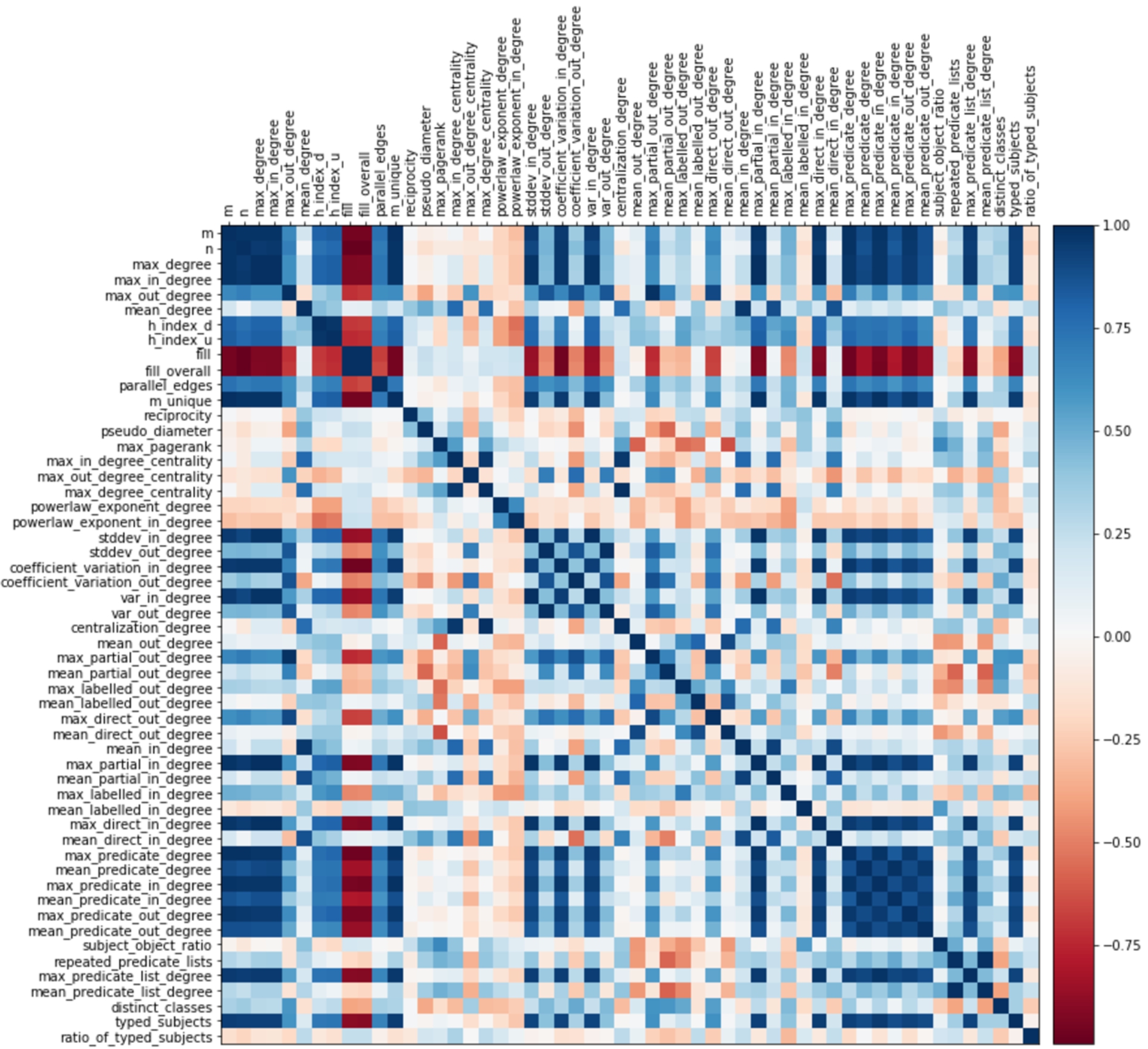
Correlation matrix. Shows the whole set of measures and their color-encoded Spearman correlation coefficient. Values close to 1.0 indicate strong positive correlation, around 0 no correlation, and close to
5.1.RQ1: What is an efficient and non-redundant set of features for characterizing RDF graphs?
5.1.1.Correlation coefficients
We first report on observations about correlation coefficients between measures. Figure 1 shows a correlation matrix of all measures with color-encoded values for the Spearman correlation coefficients. Values close to 1.0 indicate strong positive correlation, around 0 no correlation, and close to
Fig. 2.
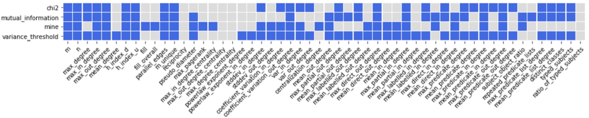
Meaningful measures according to different statistical feature selection scoring methods.
In the group of graph measures, the number of edges m and vertices n has an almost perfect correlation with (a) max_degree and (b) max_in_degree. In addition, the two measures have a strong positive mutual correlation. Due to this, other measures which employ these measures are in turn strongly correlated with each other. In particular, this can be observed for measures employing the in-degree. Descriptive statistics on the distribution of in-degrees, like var_in_degree, stddev_in_degree, and coefficient_var_in_degree, grow with the size and volume of the graphs. This does not apply for measures relating to the vertices out-degree: measures using the in-degree differ from measures using the out-degree. Most of the measures employing the out-degree do not correlate with almost any of the other measures, which makes them more descriptive. A negative correlation value implies that while values for a measure x increase, values for another measure y decrease. This is the case with measures employing the aspect of density (fill) of the graphs with increasing size n and volume m. The density of a graph also has a negative correlation to the distribution of vertex degrees, as we can see with variance, standard deviation, and coefficient of variation values. This means that the denser the graphs are (fill increases), the more homogeneous the vertex degrees of the graphs become (descriptive statistics over vertex degrees become smaller). Almost no dependencies are exhibited by mean_degree, reciprocity, diameter, centrality measures, and the powerlaw_exponents, which measures the type of distribution of vertex (in-)degrees.
In the group of RDF graph measures, there are less inter-relationships. As a group, measures employing predicate degrees, max_predicate_list_degree, together with max_partial_in_degree, max_direct_in_degree as well as the typed_subjects measure, have strong positive mutual correlations. All of the mentioned measures grow with the size n and volume m of the graphs. Some individual mutual strong positive correlations can be observed, for instance, between repeated_predicate_lists and mean_predicate_list_degree, mean_direct_in_degree and mean_in_degree and mean_partial_in_degree. As in the first group of graph measures, all “mean” in-degree measures have strong correlations among each other as well as to the mean_degree.
5.1.2.Measure selection
Figure 2 highlights the measures that were selected by the individual tests.
Overall, there is variance and no particular consensus of the statistical tests. However, there are some agreements. Looking at agreements in all tests, only 13 measures are providing information gain; only three were dismissed by all tests, i.e., two degree-centrality measures and ratio_of_typed_subjects. 16 measures have agreements in three tests (threshold was not met in one of the tests); 10 measures met the threshold in only one test. With 30 measures, the pair Chi2 and Variance Threshold has the highest number of agreements; Mutual Information and Variance Threshold agree on 27 measures. The least agreements can be found for the pair Mutual Information and MINE (18).
Fig. 3.
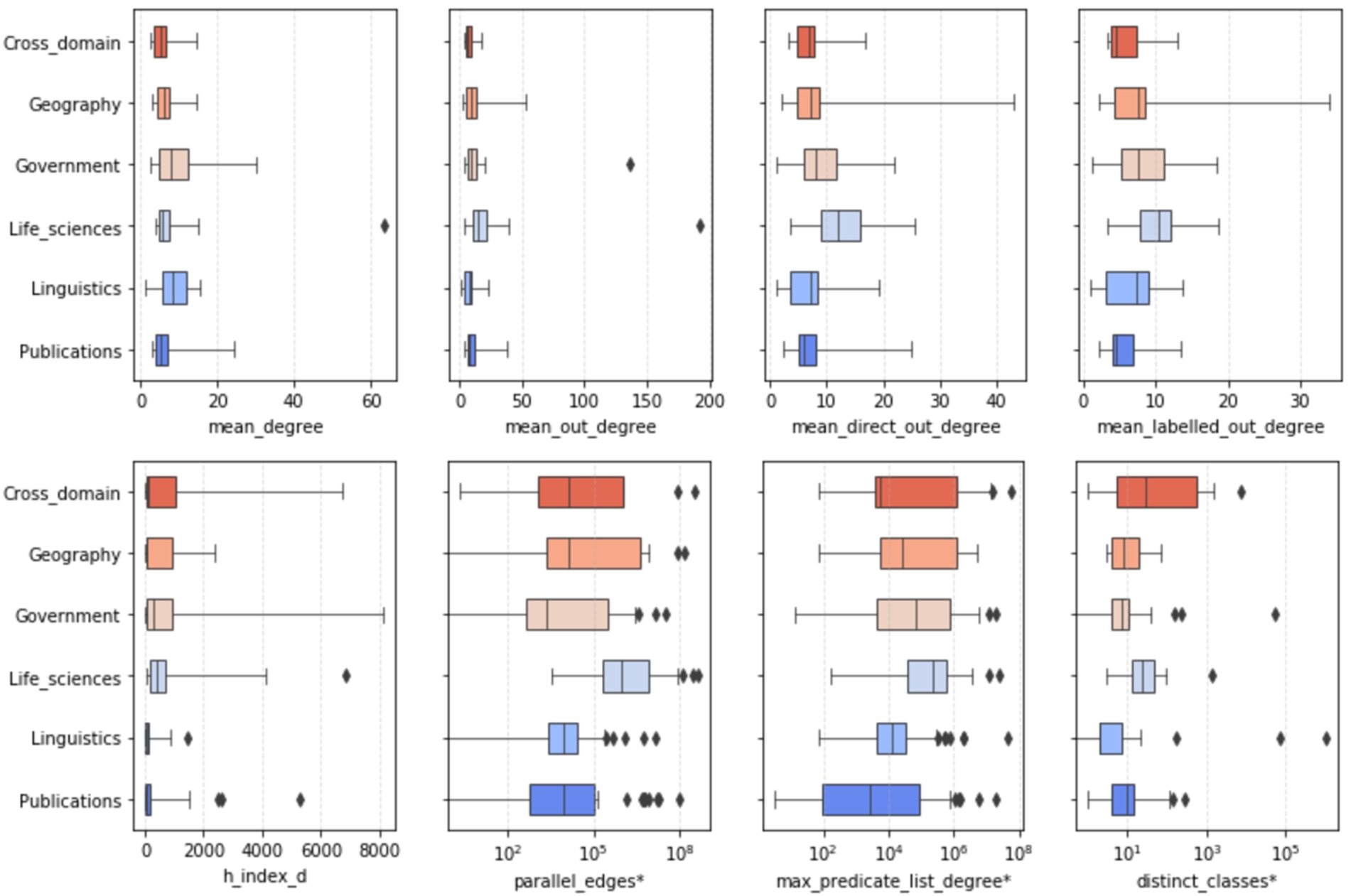
Descriptive statistics of measures sorted out by feature selection methods (top) and measures considered meaningful (bottom). ∗Indicates that x-axis is log-scaled.
5.1.3.Summary of results
With particular regard to RDF graphs and the above analysis, we conclude with the following observations:
– The larger the density, the more “stable” and homogeneous is the (in-/out-) degree distribution of vertices in the graphs.
– The larger the size and volume of the graphs, the more typed subjects become present, and the higher the number of subjects using a fixed set of predicates appears (cf. predicate degree and predicate lists measures).
– The average degree of the graphs is mainly influenced by the in-degree.
– Measures employing the distribution of out-degrees are more descriptive.
The next subsections report the results on the reduced set of meaningful measures obtained from the feature selection methods. In particular,
5.2.RQ2: Which measures and values describe and characterize knowledge domains most/least efficiently?
In order to get a sense of the variability of measures within and across knowledge domains, in this section, we look closer and report on characteristics for some individual measures first. Afterwards, we aggregate and report on variability across knowledge domains, through variance and standard deviation.
5.2.1.Characteristics of values
Figure 3 shows, by example, the distribution of values for two groups of measures. The first group at the top row shows exemplary measures which were sorted out by the feature selection approaches in Section 5.1, such as the mean total-degree and the mean out-degree; the bottom row shows exemplary features of
Regarding the mean total-degree, some categories show very similar median values, like Cross Domain, Life Sciences, and Publications. Cross Domain, Geography, Life Sciences, and Linguistics share a similar maximum value. However, regarding the outliers, Life Sciences contains a dataset that has by far the highest average degree, followed by a dataset in the Government category. The mean out-degree (outgoing predicates of subjects) is higher for most of the categories (two outliers can be observed with very high values). The boxes reveal that the majority of values are larger than the mean total-degree, which means that the mean total-degree is mainly influenced by the in-degree. This is particularly striking for datasets in the Geography and Life Sciences domains.
Fig. 4.
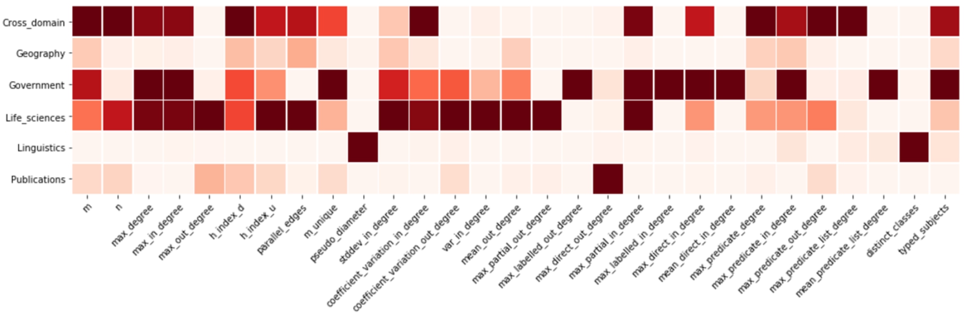
Measure variance. The lighter the color the lower the variance and the more homogeneous the values are within the corresponding category.
The last two plots in the first group show the mean_direct_out_degree and mean_labelled_out_degree measures, which describe the relationship of subjects to their average number of different objects and predicates, respectively. Overall, the number of different objects is higher than the number of predicates. The distribution of values is similar for Cross Domain and Publications, as well as for Geography and Linguistics, particularly for the predicates (mean_labelled_out_degree). Comparing mean_degree and mean_out_degree as well as mean_direct_out_degree and mean_labelled_out_degree with each other, we can see that they show very similar characteristics. Generally, the distribution of values is not symmetric (different whisker lengths of the boxes) and skewed, thus they do not follow a normal distribution. Further, there is little variability (short length of boxes).
Fig. 5.
Degree of variance across knowledge domains. A low/high value indicates low/high variance across knowledge domains. Colors encode graph measures (in light) and RDF graph measures. y-axis is log-scaled.
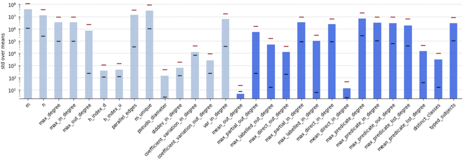
Below in Fig. 3 are exemplary measures of
Lowest spread and little variability can be found for h_index_d. The distribution of values in Cross Domain, Geography, Government is highly skewed to the right, which means that most of the values are rather low. However, there are some datasets with quite high value above 4000, e.g., in Cross Domain, Government, Life Sciences, and Publications. The largest value can be found for a dataset in the Government domain.
5.2.2.Variability of values
As a first overview, Fig. 4 shows measure variance of the datasets within the given categories as a heat-map: the lighter the color, the lower the variance and therefore the more homogeneous the corresponding values are for the corresponding category and measure.
Overall, datasets in the Life Sciences, Cross Domain, and Government (in this order) have quite heterogeneous distributions of values for a high number of measures. On the contrary, only one, two, or three measures have high variance in the Publications, Linguistics, and Geography domain (in this order). Some measures exhibit high variance in just one category and a low variance in the others. Just to name a few: max_out_degree and max_partial_out_degree in Life Sciences, pseudo_diameter and distinct_classes in Linguistics, max_labelled_in_degree and mean_predicate_list_degree in Government, max_predicate_list_degree in Cross Domain, max_direct_out_degree in Publications. These measures may be used to discriminate categories against each other very well, as their characteristical distribution of values for a particular category can be considered meaningful. In turn, some measures also exhibit a rather low variance in one or two domains and higher in the others. These are, for instance, m, h_index_d, std_in_degree in Linguistics.
Figure 5 shows the degree of variance across knowledge domains. The scores are obtained by grouping datasets by category, taking the mean of the corresponding measure for all datasets per category, and then computing the standard deviation over these means. Lowest variances across all categories can be found for mean_out_degree, mean_direct_in_degree, pseudo_diameter, both h_index measures, std_dev_in_degree, coefficient_variation_out_degree, distinct_classes, and mean_predicate_list_degree. Among the top five measures with large dispersion between categories (m, m_unique, parallel_edges, n, and max_predicate_degree) are four measures employing graph edges. The figure also includes minimum (lower stroke) and maximum (upper stroke) values. For some measures, the minimum value varies significantly from the standard deviation value. To name a few: pseudo_diameter, max_labelled_in_degree, max_predicate_list_degree, and distinct_classes.
5.2.3.Summary of results
– For the majority of the measures, the distribution of values is not normally distributed.
– The degree of variance across domains is significant for most of the measures. A low variance across domains is rather exceptional.
– Datasets in Cross Domain are heterogeneous, i.e., largest variability of the number of classes. While individual datasets have a high number of distinct classes, the variability within categories is less significant. Additionally, the number of typed subjects highly varies.
– Datasets in the Government domain have high variance in the mean degree of predicate lists, meaning that they are not homogeneous in terms of the used predicates per subject.
– Datasets in the Linguistics domain have high diameter7.
– Each knowledge domain has datasets (graphs) with unique characteristics, which enables discrimination from the other domains.
Fig. 6.
Overall measure importance while discriminating datasets (classification task (1)). Shown are mean values for all non-redundant measures
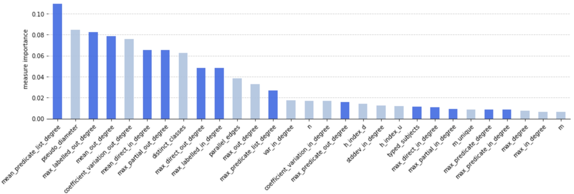
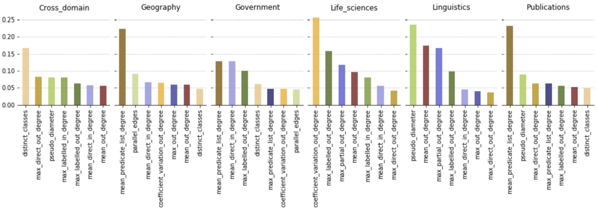
Fig. 7.
Per-category measure importance while discriminating datasets (classification task (2)). Measures are encoded by color throughout all knowledge domains.
5.3.RQ3: Which measures show the best per- formance to discriminate knowledge domains?
To recall, with this question, we aim at finding the most essential (RDF) graph measures able to discriminate knowledge domains efficiently and to measure individual measure performance. We used the approach of setting up two classification tasks with Random Forest classifiers, each tuned by hyperparameter grid-search. The first task (1) is a multiclass classification problem, the second task (2) a two-class, one-vs-rest, binary version of the first. We removed three categories and the corresponding datasets from the initially available nine knowledge domains, due to too little datasets in these categories (⩽6, cf. Table 2). The remaining data was subject to standardization with robust-scaling since earlier, we found that most features have outliers.
5.3.1.Overall measure importance
Figure 6 shows the results of classification task (1). The colors encode graph measures (in light) and RDF graph measures. The x-axis shows all measures
While the ranking shows a steadily decreasing order, the overall scores are rather low. The first 13 measures can be considered to have some impact. From the 14th value on, there is hardly a change, and the impact score is low.
Among the top 10 measures of the highest score are three graph measures (pseudo_diameter, coefficient_variation_out_degree, and distinct_classes) and seven RDF graph measures. Overall, measures employing the out-degree are favored. mean_predicate_list_degree, describing the mean number of repeated predicate used to describe subjects, has the highest score; m, describing the number of edges, the lowest.
5.3.2.Per-category measure importance
Figure 7 shows the results of classification task (2), where one can get a picture on measure performance in each of the categories. It shows per knowledge domain the top seven measures with the highest scores obtained from binary relevance method (one-vs-rest) with Random Forest classifier. Like in Fig. 6, the y-axis shows the degree of contribution to decrease impurity in the decision tree.
At first glance, we can see that the set of measures considered most important varies much across knowledge domains and that individual scores are higher than in classification task (1). Overall, there are 13 distinct measures considered here (after measure selection, the initial set of measures in
max_labelled_out_degree, mean_direct_in_degree and mean_out_degree are present in five out of six knowledge domains, although each with different scores and ranking. distinct_classes and max_direct_out_degree are present in four domains. Collecting the top two and top three measures of each knowledge domain results in having 10 and 11 distinct measures, respectively. No measure is present in exclusively one category. Hence, there seems to be no measure with particular importance in a specific category. However, distinct_classes, coefficient_variation_out_degree, and pseudo_diameter, have highest scores in Cross Domain, Life Sciences, and Linguistics, respectively. mean_predicate_list_degree is even scored highest in three domains: Geography, Government, and Publications. By far, mean_predicate_list_degree, coefficient_variation_out_degree have the highest scores in Geography, Life Sciences, and Publications, respectively. These measures can be considered most important in the corresponding categories. Their values have distinctive characteristics, which enable classifiers to discriminate datasets according to these categories. Looking closer, the results of this binary relevance task here aligns well with the single performance analysis from above: the top 10 measures from Fig. 6 are the ones which are most likely to be found in the corresponding categories in Fig. 7.
To illustrate the classification performance, Table 5 shows the scores of the binary relevance method employing the Random Forest classifier, performed on different sampling strategies as mentioned in Section 4.2.3, using the final set of features
Table 5
F-measures for the binary relevance method (one-vs-rest) with Random Forest, respecting only measures from
| Balancing strategy | F1 scores | ||
| Micro | Macro | Macro Weighted | |
| None | 0.7075 | 0.4970 | 0.6849 |
| SMOTE | 0.6896 | 0.5063 | 0.6899 |
| Rand. undersampl. | 0.5746 | 0.4043 | 0.5901 |
5.3.3.Summary of results
– To discriminate knowledge domains from each other, classifiers favor RDF graph measures over topological graph measures.
– Measures employing a max-value are favored over mean- and absolute values, like distinct_classes.
– Measures employing the out-degree are considered more important than measures employing the in-degree.
– To discriminate datasets from another, each knowledge domain considers a different set of measures as meaningful.
6.Discussion
We would like to address two major aspects exposed by the conducted experiments, namely (i) structural differences about RDF graphs from the viewpoint of graph measures, and (ii) the assessment of graph measure efficiency. The section closes up with limitations of this study.
6.1.Structural characteristics of real-world RDF datasets
The following discussion is based on the results of measure correlation coefficients (cf. Fig. 1) and measure performance scores (cf. Fig. 6 and 7).
6.1.1.General observations
By identifying effective graph features describing and discriminating RDF datasets and applying such features to LOD datasets, we gained an understanding of the topological differences of real-world datasets within distinct categories. The topology of RDF graphs (knowledge graphs more generally speaking) is distinct from other graph datasets, such as social graphs, due to the prevalence of hierarchical relations, that is, relations within the TBox (e.g. rdfs:subClassOf) or between ABox and TBox (e.g. rdf:type). This complements traversal relations and, by this means, imposes special characteristics that lead to generally higher connectivity, shorter paths, and the existence of vertex-“hubs” with high attractiveness from other vertices.
This is very well reflected in the graph measures. For example, measures like the number of edges, the maximum degree, and the maximum in-degree perfectly correlate with each other (cf. Section 5.1). Looking closer at the values for those measures reveals that 83% of the RDF graphs have vertices with a maximum in-degree being exactly equal to the maximum degree (in 94% of the cases, it is even almost equal). In most graphs, vertices representing the type (vertices with an “RDF type”-edge incident) are the ones with the highest in-degree. Such behavior of modeling, which is typical for RDF graphs and generally accepted as best practice in the RDF community, involves high connectivity of the graph’s topology. More references to the schema enhance this effect. In turn, more profound is the loss of connectivity as soon as the graph misses/loses references to the schema.
As more vertices and edges adhere to the graphs, the more heterogeneous and unstable the connectivity becomes. As a consequence, the overall density shrinks (cf. negative correlation of m, max_degree with fill) and the tendency of the topology to generate large sub-graphs having the shape of a “star” increase. Due to this and the aforementioned topological characteristic, measures employing the in-degree (some descriptive statistical measures, predicate (list-) degree measures, typed subjects, etc.) show a high correlation among each other. A stable value with growing size and volume of the graph would result in a homogeneous distribution, leading to a more stable and equally distributed connectivity of vertices among each other. The two mentioned examples can be considered being particularly RDF graph specific phenomena, which can be measured with the provided graph measures.
6.1.2.Observations within distinct categories
Vocabulary usage has a significant impact on the graph’s topology since schema and cardinality definitions are directly reflected in the graphs as options/restrictions to append vertices and edges. Thus, some measures are considered having a particular impact in individual categories, as shown in Fig. 7. Cross Domain, for instance, has a diverse and irregular vocabulary usage, which implies a large number of mixed and heterogeneous datasets, with (larger) co-occurrence of schema references and type-statements (distinct_classes). Geography and Publications report on a regular usage of vocabularies. The recurrence of a fixed set of predicates (mean_predicate_list_degree) is the main distinguishable feature of these categories. Geography additionally reports on a proportionally high ratio of parallel edges of its datasets. Inherently, datasets in Linguistics stand out with a significantly larger path length of traversal relations (pseudo_diameter7). The modeling strategy there seems fairly concise, resulting in a low average number of types and outgoing predicates/edges per subject, which is reflected by the measures mean_out_degree and max_partial_out_degree.
In general, measure importance per category has a dependency to the way how publishers, data extraction tools, and researchers describe data. For example, according to the naming pattern datasets in Linguistics are clustered into three groups: universal-dependencies-treebank-… (63 datasets), apertium-rdf-… (22 datasets), and other (37 datasets). Other examples of clusters can be found in Life Sciences (bio2rdf-…, 26 datasets) and Publications (rkb-explorer-…, 32 datasets) categories. This implies similarities of vocabulary usage, which in turn is reflected in recurrences of particular patterns in the topological structure. On account of this fact, the prevalent measure impact is also influenced by the habits of people and tools populating datasets in the individual categories.
Therefore, category-specific topological characteristics should be reflected in samples, benchmarks, or synthetic data.
6.2.Efficient RDF graph measures
The initial set of 54 measures (M) was subject to correlation coefficient analysis and feature selection methods. The size of the set reduced to 29 non-redundant measures after feature elimination (
Both experiments in Section 5.3 evaluated the same distinct set of measures. Measures below the threshold of 0.02 were considered having a particularly low level of impact. From a mixed set of graph and RDF graph measures, we identified a final efficient set of 13 measures, that is distinct and meaningful.
6.2.1.Low variability
As mentioned earlier, datasets in the individual knowledge domains show similarities in their topological structure. Thus, the set of measures considered being efficient and meaningful varies across these categories (cf. Fig. 7). According to the classifier, each of the 13 measures provides some form of information gain and meaning.
A somewhat naive intuition is that a measure with low variability is characteristic in a particular category and therefore could be considered important. The experiments show that this is not necessarily the case. In the first experiment measures with low variability (e.g., mean_out_degree, mean_direct_in_degree and pseudo_diameter) were preferred during category prediction and evaluated with higher impact scores (cf. Fig. 5 and 6). The second experiment, focusing on individual categories, showed a different situation. Measures were considered characteristic and assessed with higher impact scores as their per-category variability (shown in Fig. 4) was high. For example, mean_predicate_list_degree shows a high impact score in Government due to higher variability within and across categories (cf. Fig. 4 and 5). Similar applies for other measures, like coefficient_variation_out_degree, max_partial_out_degree, and max_labelled_out_degree. Cross Domain, for instance, employs only measures of low variability (e.g., distinct_classes, max_direct_out_degree, etc.). Thus, in our classification tasks, the classifier tries to find the right balance between a low variability across categories and a somewhat characteristic variability as a topological feature.
6.2.2.Type of measures
Compared to other types of graphs, like social networks, RDF knowledge graph topologies adhere special characteristics, such as the pervasive reference to schema elements, with rdf:type statements being the most famous reference. This peculiarity influences the assessment about the meaningfulness of measures with regard to the discrimination of categories. For example, the classification task in Section 5.3 showed that RDF graph measures are preferred and obtained higher scores over other graph invariants, such as h-index (cf. Fig. 6). Out of the 10 best performing features in classification task (1), seven were RDF graph measures. Further, measures employing the in-degree are considered less effective, due to their heterogeneous (“unstable”) value distributions. Hence, measures considering subjects and their out-degrees are considered more meaningful. Measures like the number of (parallel/unique) edges, maximal (in-) degree, maximum predicate (in-/out-) degree, and the number of typed subjects, are inherently high in variability within and across knowledge domains. Their heterogeneous character lets them be ineffective and not appropriate for dataset/category discrimination.
6.3.Limitations
There are some limitations of our experimental study that are worth to mention.
6.3.1.Size of the sample
The analysis of measure efficiency involved 280 datasets out of
6.3.2.Computational cost
Using our framework and infrastructure, we computed the described measures and study the graph topology of large state-of-the-art RDF knowledge graphs such as the English DBpedia with over 1.5B edges (cf. Table 2). However, memory consumption is a crucial bottleneck considering scale and growth of RDF graphs. Further, on graphs with a particularly large number of edges (
6.3.3.Unbalanced domain classes
In order to tackle the class imbalance of our sample, we investigated class weighting and over- and undersampling techniques on the training sample passed to the classifier. Oversampling creates synthetic datasets (no duplicates) in each class up to the number of datasets of the largest class; undersampling down-sampled all classes to the size of the smallest class.
Feature importance methods are sensitive to the data structure and the distribution of feature values, and thus all methods showed different scores for the corresponding measures. What is interesting though, the set of measures considered important was similar to a great extent, in particular the most important measure per category (e.g., mean_out_degree, mean_predicate_list_degree, pseudo_diameter, and max_labelled_out_degree). Further, the model was trained following best practices for model tuning and cross-validation-based model selection. Hence, we assume that the obtained impact ratio of the classifier for each feature is reliable.
6.3.4.Limited set of features
If one actually wanted to perform category prediction [2,26] or measure the structural similarity between RDF datasets [27], we could ask if the graph measures presented in this paper are appropriate and sufficient. As discussed earlier, vocabulary usage and the way how publishers, data extraction tools, and researchers describe data, has an impact on the graph’s topology. Employing merely ontological information of the RDF dataset is, however, not sufficient to reach acceptable prediction accuracy [2]. Our classification experiment showed that, by employing topological measures, the prediction of categories for datasets is possible. Thus, knowledge domain-related, topological, and dataset features should complement one another. Aligning and integrating other tools and features for the extraction of metadata and vocabulary usage [5] would achieve improvements in prediction accuracy. Further, the integration of measures to somewhat distinguish hierarchical and traversal relations in the graphs, as this is a key characteristic for RDF data, would be beneficial.
6.3.5.Application and generalization of the findings to other (non-RDF and non-LOD) graphs
With our framework, all of the measures in M and
However, in this work, we investigate RDF graphs only. RDF graphs are multigraphs, which may contain multiple edges between the same pair of source and target vertices, and whose use of (partly) very specialized vocabularies exposes special characteristics to the graph’s topology. Thus, the results are unlikely to be applicable to non-RDF graphs and categories outside the LOD Cloud. Moreover, although following best practice techniques for avoiding overfitting, value normalization and feature selection, classification models are very task-specific. Models are tuned towards (a) the sample of RDF datasets we obtained and analyzed from the LOD Cloud, and (b) the final set of features obtained from the feature engineering step. Thus, the generalizability of our findings to other kinds of graphs (non-RDF) is an important part of future work.
7.Conclusion and future work
We have created a framework with which one may efficiently compute topological graph measures for an arbitrary number of RDF datasets [36]. The main objective of this paper is to assess individual measure effectiveness and performance of 54 graph and RDF graph measures for RDF datasets. This is accomplished by means of statistical tests, such as the analysis of correlation coefficients, results of feature selection, analysis of variability, and a supervised classification task, in order to assess a measure’s efficiency and performance in terms of its capacity to discriminate dataset knowledge domains. For this purpose, a sample of 280 RDF datasets from nine knowledge domains was acquired from the LOD Cloud late 2017. All 280 datasets, instantiated graph objects, and values for 54 measures per graph are available for download on our website.1414 Please note that, despite following best practices for model tuning and cross-validation-based model selection, the primary aim was not to find the best classification model but to provide an understanding of feature performance, i.e., the importance of distinct graph measures in this particular task.
From a mixed set of initially 54 graph and RDF graph measures, the final set of 13 measures is actually effective, distinct, and meaningful, in order to describe RDF graphs. The majority of the measures are RDF graph-based, according to the definition in [15], and preferably employs the out-degree and outgoing edges of subjects to some extend. To discriminate categories, the following measures have the most significant impact: the average number of repeated predicate lists (mean_predicate_list_degree), the diameter of the graph (pseudo_diameter7), the maximum number of predicates with which a subject is related (max_labelled_out_degree), and the mean out-degree of the vertices (mean_out_degree).
The prevalent structure of topology is shaped by means of two mutually influencing aspects: (1) fundamental characteristics that adhere to RDF knowledge graph topologies in particular, and (2) the compliance to a standardized vocabulary. The distinctness of a measure’s impact in the individual knowledge domains implies that there are fundamental differences in the shape of topologies. An RDF dataset that is re-using a popular vocabulary will likely show characteristics that can be found in other RDF graphs. The more diverse the use of vocabularies in a dataset is, the more variety and irregularity will be found in common structural patterns of the topology. Therefore, datasets using proprietary vocabularies will differ in their structure. Hence, a group of RDF graphs with similar characteristics causes knowledge domain-dependent feature performance and impact.
Apart from the classification experiments, we also gained some understanding of the general ability to predict category labels for RDF datasets, by relying on topological measures of the graphs exclusively. The reported accuracy is comparable with other approaches and experiments, such as [2] and [26]. We came to the conclusion that this is on account of the usage of standardised and established vocabularies in the knowledge domains itself. This can be considered as being a qualitative aspect of a particular knowledge domain.
7.1.Implications
We are confident that related work in the fields of synthetic dataset generation, sampling methods, and frameworks for quality evaluation, e.g., can benefit from considering efficient topological (RDF) graph measures and category-specific assessments of the RDF graph’s topology.
– A primary goal of synthetic dataset generators is to emulate datasets and to be as close as possible to a real-world setting. Thus, topological characteristics exhibited by a particular knowledge domain are of high value. Beyond parameters like the dataset size, which is typically interpreted as the number of triples, synthetic dataset generators might employ meaningful and disregard non-efficient (RDF) graph measures, in order to target the domain of test-data generation more appropriately.
– Sampling methods aim at finding a most representative sample from an original dataset. Apart from considering qualitative aspects, like classes, properties, instances, and used vocabularies, also topological aspects of the original RDF graph should be considered. Our framework and the proposed (RDF) graph-based measures could help to evaluate the quality of a graph sample.
– Having topological measures as another group of features is beneficial for solutions that evaluate and ensure the quality of Linked Open Data, such as dataset labeling/classification tools and RDF dataset profile generators. Concerning efficient measures, each category (LOD Cloud domain class) might have its own understanding of quality, such as a large diameter for datasets in Linguistics, a lower average degree for datasets in the Life Sciences, etc. Outliers and striking values for some measures could be indicators for erroneous data or ways of modeling or using a vocabulary that is not compliant with the knowledge domain of interest.
7.2.Future work
Our intuition is that features performing well on the classification tasks also are useful, e.g., when modelling benchmark datasets, synthetic datasets or devising sampling strategies, as they are able to model dataset topology as representative for different kinds of datasets, for instance, specific dataset categories. While in this work we evaluate feature performance on the base task of distinguishing datasets, future work will deal with a more use-case driven evaluation in the context of benchmark and synthetic datasets.
Further, we plan to align graph features with features extracted by established RDF profiling tools. This widens the field of potential research and applications involving graph-based measures. For instance, we plan to improve the prediction of appropriate category labels for datasets by including features at instance- and schema-level of an RDF dataset. This enables research in the direction of quality assurance and dataset search.
In order to shape an understanding of the generalizability of our findings and to understand the graph topology through graph-based measures in other knowledge domains, we plan to include more datasets from other sources, e.g., graphs different to RDF datasets. Also, the evaluation of measures will be extended towards non-RDF graphs, with the aim to compare measure impact between these two types of graphs.
The effort for computation of some measures on very large graphs (
In terms of infrastructure, our portal is going to be updated with an upload functionality. A website visitor may then upload or provide the URL of an RDF dataset to let our framework analyze the corresponding RDF graph. By this means, we hope to collect more datasets and statistics.
In order to facilitate the access, usage, and querying of the results, we consider to represent all measures for all RDF graphs as an RDF dataset itself and import it into a publicly available SPARQL-endpoint. The RDF Data Cube Vocabulary [9] is considered for this.
Notes
2 In order for this paper to be self-contained, please note that we have re-used some paragraphs, especially for the related work in Section 2, the textual descriptions of graph measures in Section 3.2, and for the description about the acquisition of RDF datasets from the LOD Cloud in Section 4.2.1.
6 We use the notation introduced by Freeman [18], where
10 Other media type statements like html_json_ld_ttl_rdf_xml or rdf_xml_turtle_html were ignored, since they are ambiguous.
11 graph-tool, https://graph-tool.skewed.de/.
12 Our implementation mainly relies on numpy https://numpy.org/ and pandas https://pandas.pydata.org/.
References
[1] | Z. Abedjan, T. Grütze, A. Jentzsch and F. Naumann, Profiling and mining RDF data with ProLOD++, in: IEEE 30th International Conference on Data Engineering – ICDE 2014, I.F. Cruz, E. Ferrari, Y. Tao, E. Bertino and G. Trajcevski, eds, IEEE Computer Society, Los Alamitos, CA, USA, (2014) , pp. 1198–1201, ISBN 978-1-4799-3480-5. doi:10.1109/ICDE.2014.6816740. |
[2] | A. Abele, Linked data profiling: Identifying the domain of datasets based on data content and metadata, in: Proceedings of the 25th International Conference Companion on World Wide Web, J. Bourdeau, J. Hendler, R. Nkambou, I. Horrocks and B.Y. Zhao, eds, WWW ’16 Companion, International World Wide Web Conferences Steering Committee, Republic and Canton of Geneva, CHE, (2016) , pp. 287–291. ISBN 978-1-4503-4144-8. doi:10.1145/2872518.2888603. |
[3] | J. Alstott, E. Bullmore and D. Plenz, Powerlaw: A python package for analysis of heavy-tailed distributions, PloS one 9: (1) ((2014) ), e85777. doi:10.1371/journal.pone.0085777. |
[4] | D. Bachlechner and T. Strang, Is the Semantic Web a small world? in: Second International Conference on Internet Technologies and Applications – ITA 2007, (2007) , pp. 413–422. https://elib.dlr.de/47899/. |
[5] | M. Ben Ellefi, Z. Bellahsene, B. John, E. Demidova, S. Dietze, J. Szymanski and K. Todorov, RDF dataset profiling – a survey of features, Methods, Vocabularies and Applications, Semantic Web journal 9: (5) ((2018) ), 677–705. |
[6] | C. Böhm, F. Naumann, Z. Abedjan, D. Fenz, T. Grütze, D. Hefenbrock, M. Pohl and D. Sonnabend, Profiling Linked Open Data with ProLOD, in: IEEE 26th International Conference on Data Engineering Workshops – ICDEW 2010, Vol. 1: , IEEE Computer Society, Los Alamitos, CA, USA, (2010) , pp. 175–178, ISBN 978-1-4244-6522-4. doi:10.1109/ICDEW.2010.5452762. |
[7] | S. Campinas, T.E. Perry, D. Ceccarelli, R. Delbru and G. Tummarello, Introducing RDF graph summary with application to assisted SPARQL formulation, in: 23rd International Workshop on Database and Expert Systems Applications (DEXA), Vol. 1: , IEEE Computer Society, Los Alamitos, CA, USA, (2012) , pp. 261–266, ISSN 1529-4188. doi:10.1109/DEXA.2012.38. |
[8] | M.P. Consens, V. Fionda, S. Khatchadourian and G. Pirrò, S+EPPs: Construct and explore bisimulation summaries, plus optimize navigational queries; all on existing SPARQL systems, Proceedings of the VLDB Endowment (PVLDB) 8: (12) ((2015) ), 2028–2031. doi:10.14778/2824032.2824128. |
[9] | R. Cyganiak and D. Reynolds (eds), The RDF Data Cube Vocabulary, (2014) . https://www.w3.org/TR/2014/REC-vocab-data-cube-20140116/. |
[10] | R. Cyganiak, D. Wood and M. Lanthaler (eds), RDF 1.1 Concepts and Abstract Syntax, (2014) . https://www.w3.org/TR/2014/REC-rdf11-concepts-20140225/. |
[11] | J. Debattista, J. Attard, R. Brennan and D. O’Sullivan, Is the LOD Cloud at risk of becoming a museum for datasets? Looking ahead towards a fully collaborative and sustainable LOD cloud, in: Companion Proceedings of the 2019 World Wide Web Conference – WWW 2019, S. Amer-Yahia, M. Mahdian, A. Goel, G.-J. Houben, K. Lerman, J.J. McAuley, R. Baeza-Yates and L. Zia, eds, WWW ’19, ACM Digital Library, New York, NY, USA, (2019) , pp. 850–858, ISBN 978-1-4503-6675-5. doi:10.1145/3308560.3317075. |
[12] | J. Debattista, C. Lange, S. Auer and D. Cortis, Evaluating the quality of the LOD Cloud: An empirical investigation, Semantic Web journal 9: (6) ((2018) ), 859–901. doi:10.3233/SW-180306. |
[13] | J. Demter, S. Auer, M. Martin and J. Lehmann, LODStats – an extensible framework for high-performance dataset analytics, in: Knowledge Engineering and Knowledge Management, A. ten Teije, J. Völker, S. Handschuh, H. Stuckenschmidt, M. d’Aquin, A. Nikolov, N. Aussenac-Gilles and N. Hernandez, eds, Lecture Notes in Computer Science, Vol. 7603: , Springer, Berlin, Heidelberg, (2012) , pp. 353–362, ISBN 978-3-642-33876-2. doi:10.1007/978-3-642-33876-2_31. |
[14] | L. Ding and T. Finin, Characterizing the Semantic Web on the Web, in: The Semantic Web – ISWC 2006, I. Cruz, S. Decker, D. Allemang, C. Preist, D. Schwabe, P. Mika, M. Uschold and L.M. Aroyo, eds, Lecture Notes in Computer Science, Vol. 4273: , Springer, Berlin, Heidelberg, (2006) , pp. 242–257, ISBN 978-3-540-49055-5. doi:10.1007/11926078_18. |
[15] | J.D. Fernández, M.A. Martínez-Prieto, P. de la Fuente Redondo and C. Gutiérrez, Characterising RDF data sets, Journal of Information Science 44: (2) ((2018) ), 203–229. doi:10.1177/0165551516677945. |
[16] | B. Fetahu, S. Dietze, B.P. Nunes, M.A. Casanova, D. Taibi and W. Nejdl, A scalable approach for efficiently generating structured dataset topic profiles, in: The Semantic Web: Trends and Challenges – ESWC 2014, V. Presutti, C. d’Amato, F. Gandon, M. d’Aquin, S. Staab and A. Tordai, eds, Lecture Notes in Computer Science, Vol. 8465: , Springer, Cham, (2014) , pp. 519–534, ISBN 978-3-319-07442-9. doi:10.1007/978-3-319-07443-6_35. |
[17] | A. Flores, M.-E. Vidal and G. Palma, Graphium chrysalis: Exploiting graph database engines to analyze RDF graphs, in: The Semantic Web: ESWC 2014 Satellite Events, V. Presutti, E. Blomqvist, R. Troncy, H. Sack, I. Papadakis and A. Tordai, eds, Lecture Notes in Computer Science, Vol. 8798: , Springer, Cham, (2014) , pp. 326–331, ISBN 978-3-319-11955-7. doi:10.1007/978-3-319-11955-7_43. |
[18] | L.C. Freeman, Centrality in social networks: Conceptual clarification, Social Networks 1: (3) ((1979) ), 215–239. doi:10.1016/0378-8733(78)90021-7. |
[19] | R. Gil and R. García, Measuring the Semantic Web, in: Advances in Metadata Research, S. Sanchez-Alonso, ed., Proceedings of MTSR 2005, Vol. 1, Rinton Press, Princeton, NJ, USA, (2006) , pp. 72–77, ISBN 1-58949-053-3. |
[20] | C. Gutiérrez, C.A. Hurtado, A.O. Mendelzon and J. Pérez, Foundations of Semantic Web databases, Journal of Computer and System Sciences 77: (3) ((2011) ), 520–541. doi:10.1016/j.jcss.2010.04.009. |
[21] | A. Haller, J.D. Fernández, M.R. Kamdar and A. Polleres, What are links in Linked Open Data? A characterization and evaluation of links between knowledge graphs on the Web, Journal of Data and Information Quality 12: (2) ((2020) ), 9. doi:10.1145/3369875. |
[22] | J.E. Hirsch, An index to quantify an individual’s scientific research output, Proceedings of the National Academy of Sciences 102: (46) ((2005) ), 16569–16572. doi:10.1073/pnas.0507655102. |
[23] | A. Hogan, A. Harth, A. Passant, S. Decker and A. Polleres, Weaving the Pedantic Web, in: Proceedings of the Linked Data on the Web Workshop – LDOW 2010, C. Bizer, T. Heath, T. Berners-Lee and M. Hausenblas, eds, CEUR Workshop Proceedings, Vol. 628: , CEUR-WS.org, Raleigh, North Carolina, USA, (2010) , ISSN 1613-0073. |
[24] | W. Hu, H. Qiu and M. Dumontier, Link analysis of life science linked data, in: The Semantic Web – ISWC 2015, M. Arenas, O. Corcho, E. Simperl, M. Strohmaier, M. d’Aquin, K. Srinivas, P.T. Groth, M. Dumontier, J. Heflin, K. Thirunarayan and S. Staab, eds, Lecture Notes in Computer Science, Vol. 9367: , Springer, Cham, (2015) , pp. 446–462, ISBN 978-3-319-25010-6. doi:10.1007/978-3-319-25010-6_29. |
[25] | S. Khatchadourian and M.P. Consens, ExpLOD: Summary-based exploration of interlinking and RDF usage in the Linked Open Data cloud, in: The Semantic Web: Research and Applications – ESWC 2010, L. Aroyo, G. Antoniou, E. Hyvönen, A. ten Teije, H. Stuckenschmidt, L. Cabral and T. Tudorache, eds, Lecture Notes in Computer Science, Vol. 6089: , Springer, Berlin, Heidelberg, (2010) , pp. 272–287, ISBN 978-3-642-13489-0. doi:10.1007/978-3-642-13489-0_19. |
[26] | S. Lalithsena, P. Hitzler, A.P. Sheth and P. Jain, Automatic domain identification for Linked Open Data, in: Web Intelligence, Vol. 1: , IEEE Computer Society, Los Alamitos, CA, USA, (2013) , pp. 205–212, ISBN 978-1-4799-2902-3. doi:10.1109/WI-IAT.2013.206. |
[27] | P. Maillot and C. Bobed, Measuring structural similarity between RDF graphs, in: Proceedings of the 33rd Annual ACM Symposium on Applied Computing, H.M. Haddad, R.L. Wainwright and R. Chbeir, eds, SAC ’18, ACM Digital Library, New York, NY, USA, (2018) , pp. 1960–1967, ISBN 9781450351911. doi:10.1145/3167132.3167342. |
[28] | N. Mihindukulasooriya, M. Poveda-Villalón, R. García-Castro and A. Gómez-Pérez, Loupe – an online tool for inspecting datasets in the Linked Data Cloud, in: Proceedings of the ISWC 2015 Posters & Demonstrations Track, S. Villata, J.Z. Pan and M. Dragoni, eds, CEUR Workshop Proceedings, Vols 1486: , CEUR-WS.org, (2015) , ISSN 1613-0073. |
[29] | M.E.J. Newman, Networks: An Introduction, Oxford University Press, (2010) , ISBN 978-0-198-80509-0. |
[30] | L. Page, S. Brin, R. Motwani and T. Winograd, The PageRank Citation Ranking: Bringing Order to the Web, Technical Report, 1999–66, Stanford InfoLab (1999), Previous number = SIDL-WP-1999-0120. http://ilpubs.stanford.edu/422/. |
[31] | S. Qiao and Z.M. Özsoyoğlu, RBench: Application-specific RDF benchmarking, in: Proceedings of the 2015 ACM SIGMOD International Conference on Management of Data, SIGMOD ’15, ACM Digital Library, New York, NY, USA, (2015) , pp. 1825–1838, ISBN 978-1-450-32758-9. doi:10.1145/2723372.2746479. |
[32] | M. Schmachtenberg, C. Bizer and H. Paulheim, Adoption of the Linked Data Best practices in different topical domains, in: The Semantic Web – ISWC 2014, P. Mika, T. Tudorache, A. Bernstein, C. Welty, C.A. Knoblock, D. Vrandečić, P.T. Groth, N.F. Noy, K. Janowicz and C.A. Goble, eds, Lecture Notes in Computer Science, Vol. 8796: , Springer, Cham, (2014) , pp. 245–260, ISBN 978-3-319-11964-9. doi:10.1007/978-3-319-11964-9_16. |
[33] | G. Sejdiu, I. Ermilov, J. Lehmann and M.N. Mami, DistLODStats: Distributed computation of RDF dataset statistics, in: The Semantic Web – ISWC 2018, D. Vrandečić, K. Bontcheva, M.C. Suárez-Figueroa, V. Presutti, I. Celino, M. Sabou, L.-A. Kaffee and E. Simperl, eds, Lecture Notes in Computer Science, Vol. 11137: , Springer, Cham, (2018) , pp. 206–222, ISBN 978-3-030-00668-6. doi:10.1007/978-3-030-00668-6_13. |
[34] | Y. Theoharis, Y. Tzitzikas, D. Kotzinos and V. Christophides, On graph features of Semantic Web schemas, IEEE Transactions on Knowledge & Data Engineering 20: (5) ((2008) ), 692–702. doi:10.1109/TKDE.2007.190735. |
[35] | D.J. Watts, Networks, dynamics, and the small-world phenomenon, American Journal of Sociology 105: (2) ((1999) ), 493–527. doi:10.1086/210318. |
[36] | M. Zloch, M. Acosta, D. Hienert, S. Dietze and S. Conrad, A software framework and datasets for the analysis of graph measures on RDF graphs, in: The Semantic Web, P. Hitzler, M. Fernández, K. Janowicz, A. Zaveri, A.J.G. Gray, V. López, A. Haller and K. Hammar, eds, Lecture Notes in Computer Science, Vol. 11503: , Springer, Cham, (2019) , pp. 523–539, ISBN 978-3-030-21348-0. doi:10.1007/978-3-030-21348-0_34. |
[37] | M. Zneika, D. Vodislav and D. Kotzinos, Quality metrics for RDF graph summarization, Semantic Web journal 10: (3) ((2019) ), 555–584. doi:10.3233/SW-190346. |


