
Digital radiography image denoising using a generative adversarial network
Abstract
Statistical noise may degrade the x-ray image quality of digital radiography (DR) system. This corruption can be alleviated by extending exposure time of detectors and increasing the intensity of radiation. However, in some instances, such as the security check and medical imaging examination, the system demands rapid and low-dose detection. In this study, we propose and test a generative adversarial network (GAN) based x-ray image denoising method. Images used in this study were acquired from a digital radiography (DR) imaging system. Promising results have been obtained in our experiments with x-ray images for the security check application. The Experiment results demonstrated that the proposed new image denoising method was able to effectively remove the statistical noise from x-ray images, while kept sharp edge and clear structure. Thus, comparing with the traditional convolutional neural network (CNN) based method, the proposed new method generates more plausible-looking images, which contains more details.
1Introduction
X-ray digital radiography (DR) is an essential method for non-destructive detection in security check and medical imaging examination, which can show internal details and structures of objects. However, X-ray images may be corrupted by statistical noises, which seriously deteriorates the quality of X-ray images and raises the difficulty of diagnosis [1, 2]. Although extending exposure time of detectors and increasing the intensity of radiation are effective ways to mitigate the problem, it increased the complexity and detection time. Thus, it is highly desirable to suppress the statistical noise while using the same detection time.
The statistical noises in x-ray images are non-Gaussian, spatial-variant and related to surrounding structures, which are hard to eliminate while maintaining the surrounding details [3] Nonlinear techniques have been proven to be a more effective way to suppress the noise compared to linear approaches. However, the denoised image is still too blurry to diagnose because of the loss of high-frequency details such as edges and texture [4, 5].
Recently, various supervised machine learning methods have been proposed to reduce noise of x-ray images by learning the relation between a noise-contaminated image INC and its corresponding noise-free image INF from the training dataset [6, 7]. Especially, the deep learning based denoising methods in x-ray images has shown the excellent performance and achieved impressive successes [8–12].
Despite the great achievement that have been made, most of deep learning based methods train convolutional neural networks to minimize the mean squared error (MSE) between thevnetwork output and the ground truth as the loss function. However, the MSE is quite different from human perception and is not a perfect criterion for image quality. As a result of MSE minimization, the denoised image may be overly smooth and lose details, which limits the diagnosis of smaller structures in denoised images. Moreover, the noise-contaminated images in training datasets are often generated by adding noise to noise-free images, which is quite different from real application. The difference between training data and real data is also a limitation of performance.
In this work, we propose to train a generative adversarial network [13] for noise reduction of x-ray images. The proposed method is trained on an x-ray image dataset, in which the noise-contaminated images are acquired by digital radiography system with shorter exposure time while the corresponding noise-free images were acquired with longer exposure time. The training dataset is close to the images from real applications, which is helpful to the performance. The proposed network consists of a generator network and a discriminator network. The generative network G is trained to generate images from input noise-contaminated images, while the discriminator network is trained to distinguish the noise-free reference images from the outputs of generator network, which is an optimization target of the generator network. The generator network is constrained with MSE, the prediction of total variation loss and image features extracted by a convolution neural network (CNN), which forces the generated images to be more realistic. The contributions of different optimization targets have been evaluated in the following experiments.
2Background
2.1X-ray image denoising
Major sources of noise in an x-ray imaging system are inherent noise and x-ray quantum noise, which follows the Gaussian distribution and Poisson distribution respectively. Among them, the quantum noise can be reduced by increasing the intensity or exposure of x-ray. However, the limitation of dose and exposure time increases the Poisson noise of the x-ray images. Hence, x-ray image denoising is key to DR image processing. Over past decades, a large number of methods have been proposed to remove image noise. In order to discriminate the clean image from its noise-contaminated image, researchers have proposed a number of methods based on various image priors, such as BM3D [14] and WNNM [15]. As an alternative, instead of employing hand-crafted image priors, deep learning based denoising methods extract the image features and learn the mapping function automatically, which show higher performance than traditional denoisers. Recent studies have provided promising results by applying CNN based denoisers to X-ray images [8–10]. The CNNs are trained using normal-dose images and their corresponding low-dose images generated by adding Poisson noises based on physical models. Generative adversarial network has also been used to produce more realistic images for noise reduction in low-dose CT [11, 12].
2.2Convolution neural networks
Convolution neural network, suitable for image processing, has shown great performance in image classification and is gaining popularity in other computer vision fields [16, 17]. It was shown that deeper network architectures have the potential to increase the networks accuracy and lead to a stronger learning capacity [18]. To efficiently train a deeper network, the residual blocks and skip-connections introduced by He and colleagues [19] are often adopted, which is an effective way to solve the vanishing/exploding gradient problem by forcing the network to predict the residual information.
As a type of CNN, generative adversarial network (GAN) is widely used for image generation [20] and style transfer problem [21]. A GAN framework consists of a generative network G and a discriminator network D that are trained simultaneously. The generative network G is trained to generate images while the discriminator network D is trained to discriminate between real and generated images. In addition to unsupervised learning problem, GANs have also been used for image super-resolution [22] and image enhancing problem [23].
3Methods
The aim of DR image denoising problem is to generate a high-quality denoised DR image ID (denoised image) from a noise-contaminated image INC. The noise-free image INF is the learning target of ID, which is only available during training. In this study, we trained a generating denoising function Fw,b based on generative adversarial networks (DNGAN) parameterized by weights w and bias b that generate a denoised image ID as similar to the noise-free image INF as possible from a noise-contaminated image INC. Given the training set
(1)
Where P denotes the perceptual loss function as detailed in section 3.1.
3.1Perceptual loss function
The perceptual quality of the DR images is determined by three parts: gray values, texture quality and content quality. The loss functions of each part are specially designed to ensure the generated images are perceptually satisfactory.
3.1.1MSE loss
For the low-level computer vision problem, mean squared error (MSE) is a typical loss function, which minimizes the pixel-wise differences between input and label images. MSE loss can be written as
(2)
However, the MSE loss has difficulty representing perceptually differences and results in the loss of high-frequency details such as textures. Thus, the MSE loss is only used for gray value constraint of the generated image.
3.1.2Adversarial loss
Inspired by [23], we built generative adversarial networks (GANs) to predict whether the input image is a real noise-free image. The noise-free images contain rich high-frequency details, thus the introduction of adversarial loss encourages the generator network to generate texture details to fool the discriminator network. To output more perceptually satisfying images, the adversarial loss is defined based on the probabilities of the discriminator
(3)
where D denote output of discriminator network.
3.1.3Content loss
According to Simonyan and Zisserman [24], the outputs of the pre-trained neural network can be used to extract the high-level feature of the images and address content loss of the image, which helps to produce images with perceptual similarity. Compared with VGG-19 network, the Resnet-34 network is faster while gains a better performance in recognition [19]. Thus in this study, we define the content loss based on the activation maps produced by the ReLU layers of the pre-trained Resnet-34 network instead of VGG-19 network. The content loss is defined as Euclidean distance between feature representations of the denoised images and noise-free images:
(4)
where R is the feature maps obtained by Resnet-34, CR,HR,WR denotes the number, height and width of the feature maps.
3.1.4Total variation loss
Although the adversarial loss forces the generator network outputs high-frequency information, which makes image more perceptually satisfying, the generated high-frequency information is quite different from ground truth image, which can be observed in [22]. Sometimes, the generated artifacts will be harmful to the information of the image. To compress the artifacts of the generated images, total variation (TV) is also introduced in our method:
(5)
H,W denotes the number, height and width of the generated image
According to our experimental experience, our final loss is defined as
(6)
where the content loss is based on the features extracted by the pre-trained Resnet-34 model.
3.2Network architectures
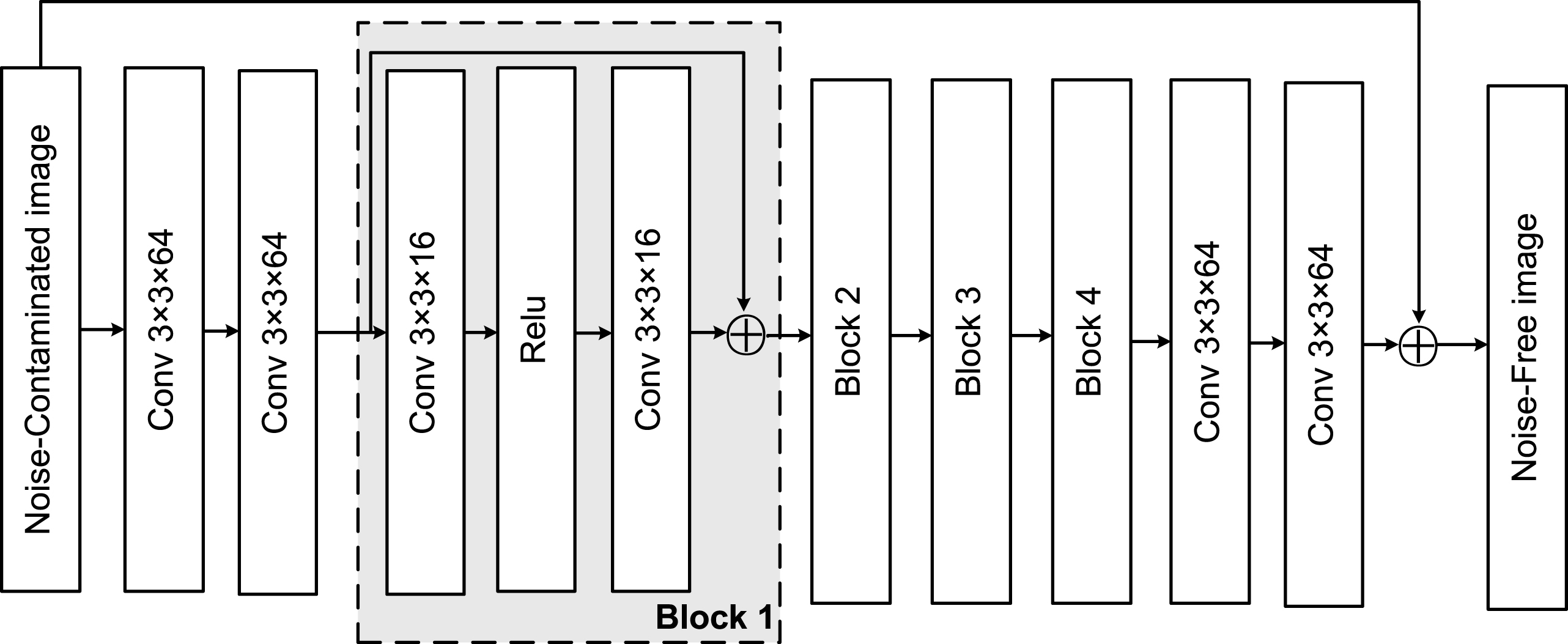
The generator network G generates the noise-contaminated DR images into denoised DR images, which are illustrated in Figure 1. The generator network consists of 12 cascading convolutional layers, which are trained to learn the residual images of label images and input images. Inner connections are introduced in each block to preserve the information and ease the training difficulty. To reduce the computational complexity while maintaining a good performance, the network adopts a bottleneck architecture, of which the number of feature maps of the first, middle and last two layers are 64. Following the practical setting in CNN for low-level computer vision problems, 3×3 kernels were used in each convolutional layer and Rectified Linear Unit (ReLU) is used as the activation function.
Fig. 1
The structure of the generator network.
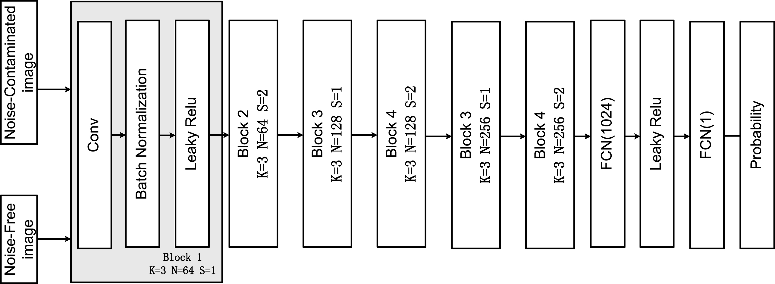
The discriminator CNN D is trained to discriminate the generated images and ground truth images. As shown in Fig. 2, D has 4 convolutional blocks and 2 fully-connected layers. Each convolutional block consists of a convolutional layer, a batch normalization layer and a leaky Relu activation layer. The kernel size K of the convolutional layers are 3×3 and the number of filters N is increased from 64 to 256. The strides of convolutional layers S are 2 to reduce the image resolution when the number of features is doubled. A single output fully-connected layer is applied to the outputs of the last fully connected layer containing 1024 neurons and produces a probability that the input image is a noise-free image.
Fig. 2
The structure of the discriminator network.
3.3Dataset
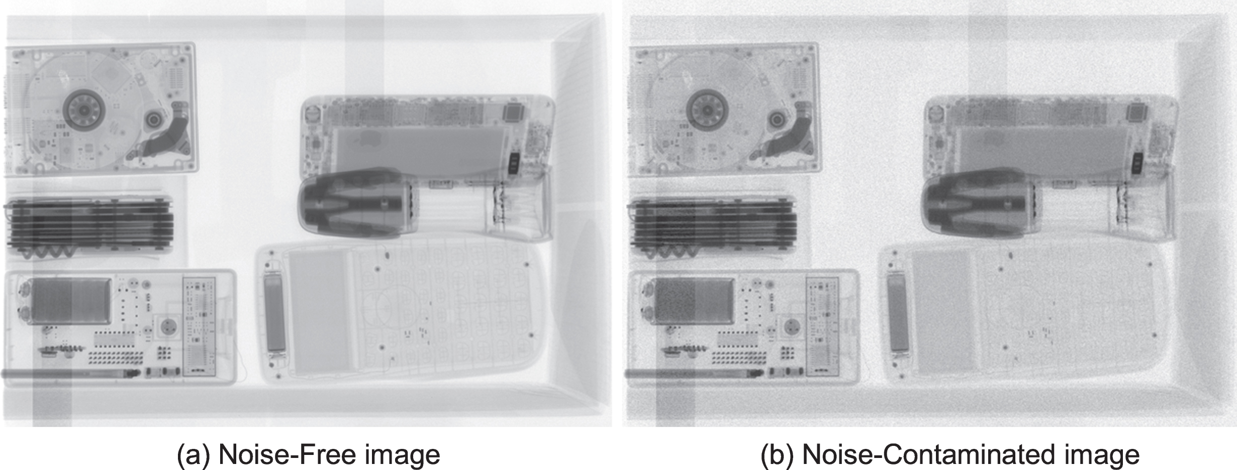
We used a real digital radiography dataset acquired using an X-ray machine with tube voltage of 210 kVp and 2048*2048 panel detectors with 1.5 mm resolution. According to Kim et al. [25], increasing the variety of input samples can improve the generalization ability of the neural network. The training dataset contains 50 noise-free images and 200 corresponding noise-contaminated images, which is sufficient for the low-level computer vision problem according to Dong et al. [26]. In our experiments, the 50 noise-free images are obtained with a tube current of 100 mAs, which can be considered as ground truth images for the neural network. The 200 noise-contaminated images are generated by the same objects obtained with tube current reduced to 2/5 mAs by reducing the exposure time and current. Figure 3 shows typical noise-free image and corresponding noise-contaminated image of the dataset.
Fig. 3
Training pairs in the dataset.
4Experiments and results
Data augmentation techniques including rotation, scaling and flipping are applied to the dataset to generate 320 images for training. Training CNN on whole DR images is infeasible. Thus, patches of size 64×64 are randomly cropped from the DR images. As a result, 40960 pairs of patches are used for training, while 10240 pairs are used for validation.
4.1Training details
The proposed model is trained using the Tensorflow package on a workstation with an Intel i7 6800 k CPU and a GTX1080 GPU. The parameters of the networks were optimized using the Adam [27] optimizer with a setting of β1 = 0.9, β2 = 0.9, learning rate of 10-4 and batch size of 16. The generator network is initialized with MSE loss after 100 epochs training, while the Resnet-34 network and the discriminator network are trained for 2000 epochs. The methods contain the networks with MSE individually (DNGAN-MSE), adversarial loss (DNGAN-ADV) individually, without content loss (DNGAN-WORES), without MSE loss (DNGAN-WOMSE) and the network without TV loss (DNGAN-WOTV).
The convergence curves of the different methods during the training process for the validation dataset are shown in Fig. 4. It can be noted that the Resnet loss amounts to the most part of the perceptual loss, while the other three losses amount similar shares. Compared with DNGAN-WOTV, the DNGAN convergent more smoothly while gets lower Resnet loss and MSE loss. The total variation loss of the DNGAN-WORES is volatile, which indicates some artifacts are associate with the absence of the Resnet loss. The DNGAN gets the lowest Resnet loss and MSE loss, which also can be observed in the generated images.
Fig. 4
Convergence curves during the training process of four networks.
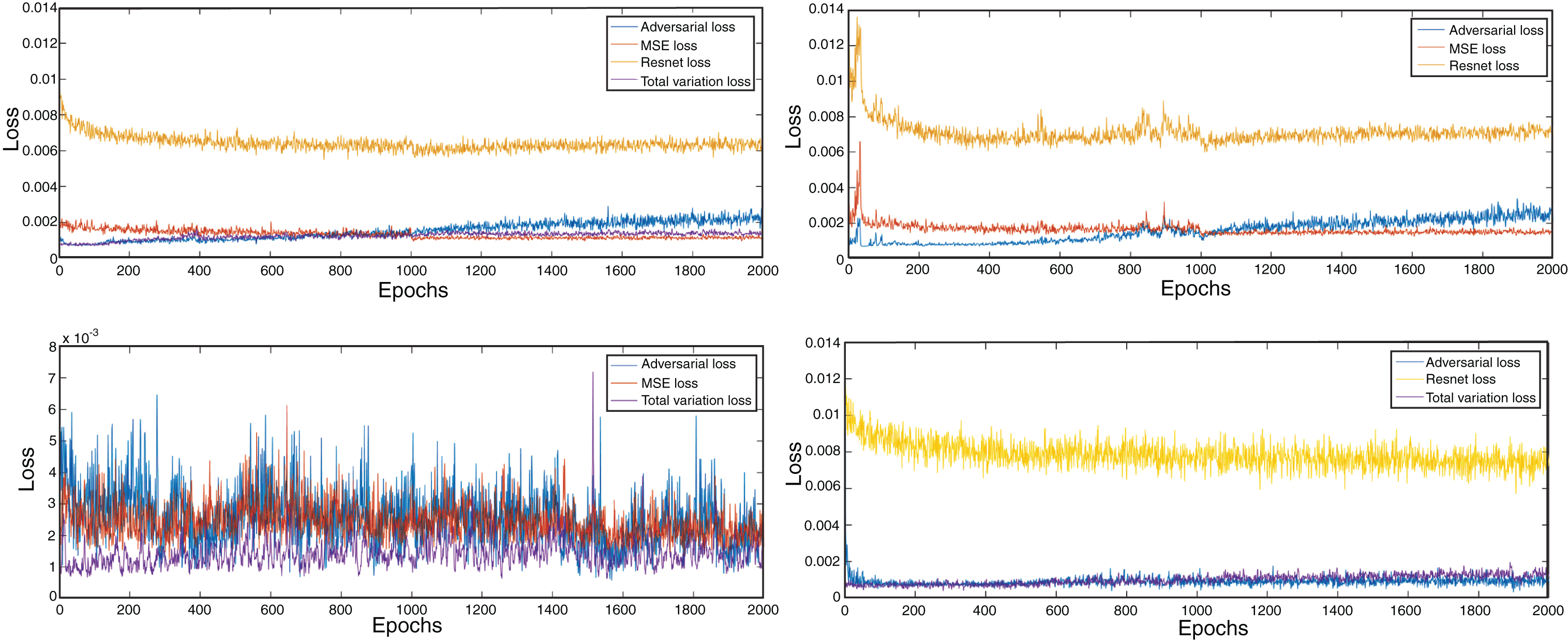
These observations suggest that the model trained with the MSE loss function can be regarded as a low-pass filter, which suppress the noise of images while leads to the over-smoothed effect of the generated images. The introduction of the adversarial loss increases the gradients of generated images by adding noises, which are quite different from image details. To release the problem, high-level features extracted from a pre-trained network such as VGG net or Resnet make the noises to be similar with the image details. The total variation loss can be used to suppress the generated noise while maintains the structure of images.
4.2Quantitative metrics
As a challenge of computer vision, image quality assessment remains an open problem. Most of traditional perceptual image quality metrics such as PSNR and SSIM are based on per-pixel measurement, which are too simple to account for human perception. For example, blurred images could get high PSNR and SSIM values while get worse visual effect, which also can be observed in following experiments.
Most recently, [28] proposed a perceptual similarity metric based on deep features which extracted by convolutional networks. The perceptual distance in the space of deep feature is used to measure the similarity of two images, which closed human judgment. The metric is evaluated using a large-scale dataset containing human judgments and proved to outperform previous metrics, which is better match human perception.
For quantitative analysis PSNR, SSIM and perceptual distance proposed in [28] are adopted to assess the quality of generated images in this work. It is worth noting that a generated image with lower perceptual distance between reference images means a better similarity with ground truth image.
4.3Denoising results and analysis
To validate the advantage of the proposed methods, the different methods are tested on a test dataset, which contains five image patches cropped from entire images. The denoising results of different loss function are shown in Figs. 5 and 6, in which details are marked and zoomed at the bottom of the results. Traditional denoising method BM3D is adopted in this test as a contrast. Peak-to-noise ratio (PSNR), structural similarity (SSIM) and perceptual distance from the reference image (PDR) of each result are calculated for quantitative evaluation and are summarized in Table 1.
Fig. 5
Denoising results of image 1.
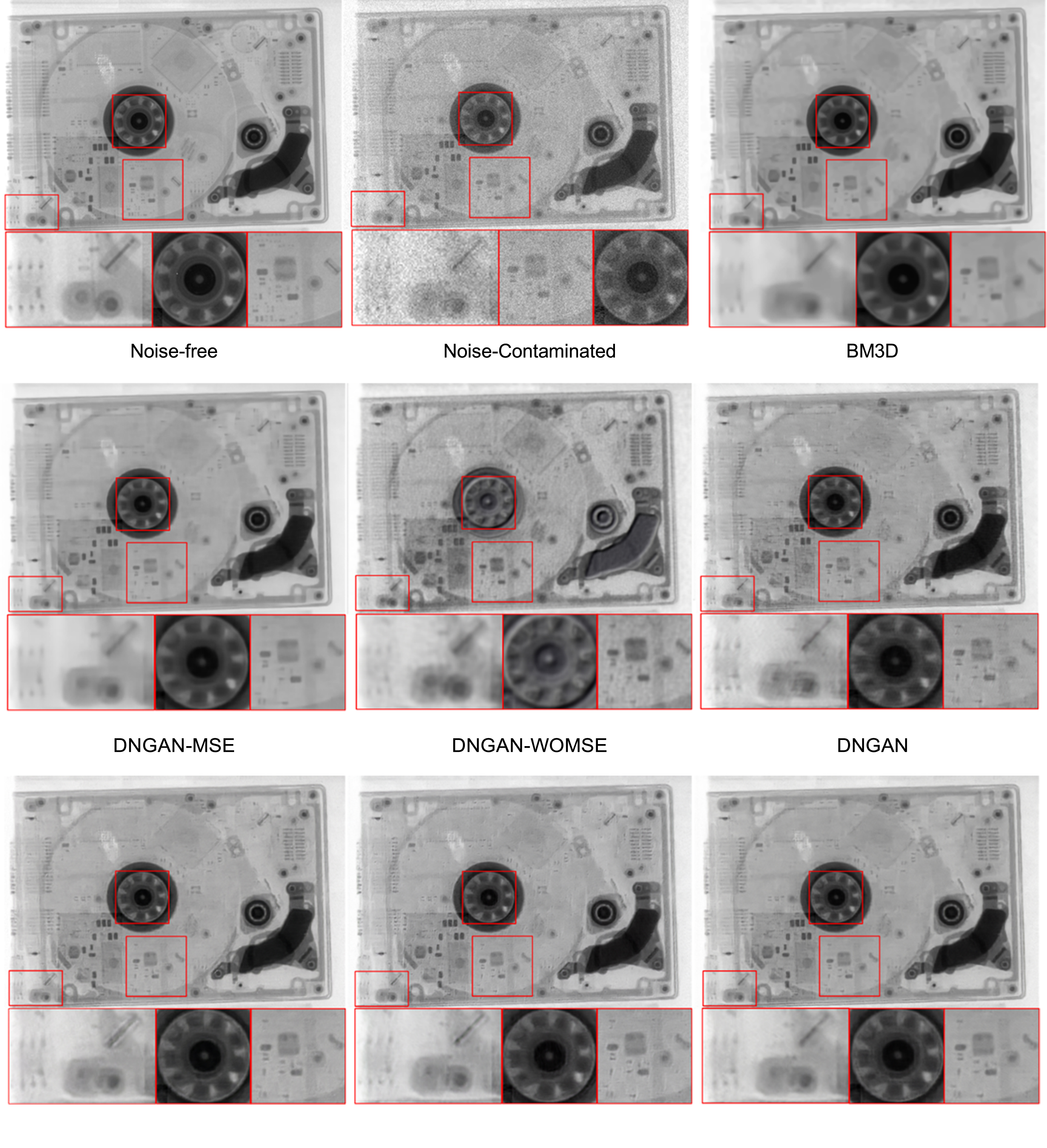
Fig. 6
Denoising results of image 2.
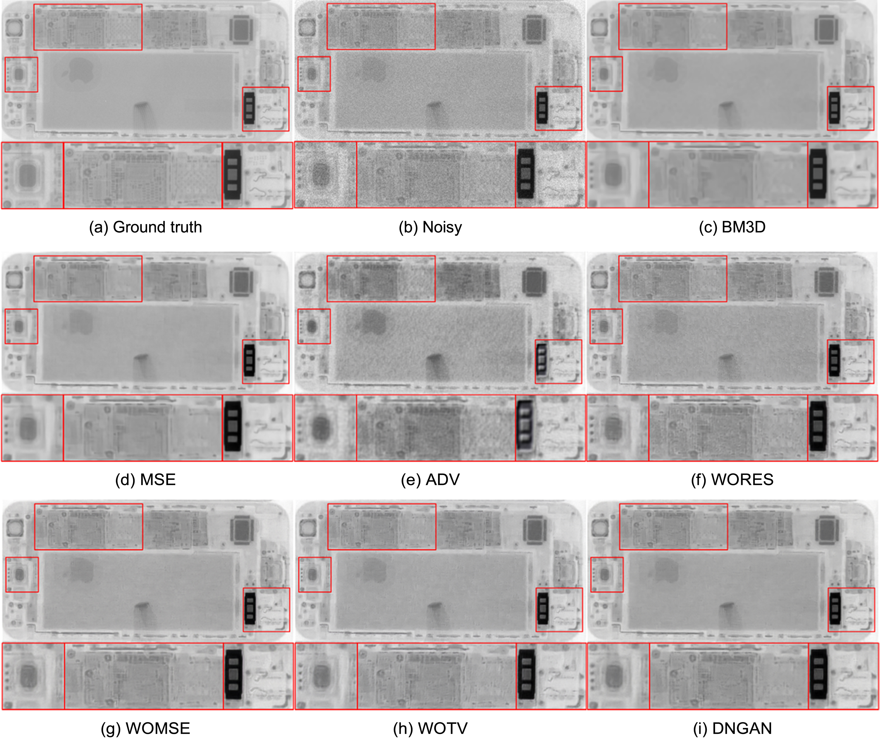
Table 1
Average quantitative results of different results
| Method | Noisy | BM3D | MSE | ADV | WORES | WOMSE | WOTV | DNGAN |
|---|---|---|---|---|---|---|---|---|
| PSNR | 24.15 | 33.18 | 35.04 | 25.83 | 31.73 | 30.86 | 32.76 | 32.95 |
| SSIM | 0.387 | 0.904 | 0.913 | 0.760 | 0.887 | 0.892 | 0.890 | 0.894 |
| PDR | 0.344 | 0.119 | 0.105 | 0.143 | 0.067 | 0.045 | 0.051 | 0.043 |
Since PSNR criterion is equivalent to MSE, it is to be expected that DNGAN-MSE gets the best results in PSNR. However, DNGAN-MSE performs worse in PDR while the details of images are blurry and the edges tends to be overly smooth, which indicates the generated images are not perceptually convincing. In the marked region of images, the details are too blur compared with noise-free image, which is caused by the difference between MSE loss with perceptual loss. In contrast, the DNGAN-ADV gets the sharpest results, however it performs the worst in PSNR and SSIM. What’s more, the structures and details of the generated image are distorted, which indicates that the adversarial loss tends to create high-frequency artifacts and cannot be perception function loss alone. The problem is released while the content loss or MSE loss is used to restrict the adversarial loss, the artifacts are restrained and MSE and SSIM values of the generated images are higher than DNGAN-ADV. The result shows that MSE and VGG regularization play important roles in perceptual loss function.
Compared with DNGAN-WOMSE, the DNGAN-WORES obtains a similar performance in MSE and SSIM while better in PDR, which generates clearer and more perceptual convincing images. Sharp edges and clear structures can be observed in the marked regions of the images generated by DNGAN-WORES, which are more perceptually similar with the reference images compared with DNGAN-ADV and DNGAN-MSE. The result may indicate that the high-level features extracted by pre-trained Resnet-34 integrate the human perception into the generated images, which is helpful to the generator network to output more visually satisfying results while achieve a better MSE result. However, the DNGAN ranks better in all the metrics than DNGANN-WOMSE and get the best PDR result, while the details of the generated images are more similar with the ground truth, which indicates the MSE loss is an essential part of the perceptual function.
The DNGAN-WOTV also generates sharp edges, however, some spots and streaks which doesn’t exist on the reference images can be observed. The artifacts are generated by the optimization of adversarial loss and reduces the perceptual effect of the generated images. To compress the artifacts, the total variation loss is introduced as a part of the perceptual loss function of the DNGAN.
As a result, the DNGAN ranks the best in PDR and gets most perceptually satisfying result while keeping an excellent PSNR and SSIM performance.
4.4Weights setting of the function loss
In the section 3.1, we discuss about the perceptual loss function, in which the weight setting of each part significantly affects the generated results. For instance, a higher setting of the total variation loss may over smooth the generated images, while a lower setting may be ineffective.
In this section, PDR is adopted to measure the effect of different settings of weights. Due to the perceptual loss function contains four hyper-parameters, we keep the losses with similar values and change a single weight of parameters with factor 0.2, 0.5, 1, 2 and 5. According to the loss function described in section 3.1, the MSE loss and the total variation loss are in the same order. The adversarial loss is three orders higher than the MSE loss while the content loss is about 40 times higher based on the experiments. To keep a similar contribution of each the weights of loss function is initialized as P = LMSE + 0.025 * LContent + 0.01 * LADV + 0.5 * LTV
Each test is trained after 500 epochs. The results are shown in Fig. 7 and Table 2, from which we can observe that a higher weight of content loss could improve the quality of generated images. The factor of TV loss is better set as 0.5, while factors of the MSE loss and the adversarial loss are better set as 1. As a result, the perceptual function should be set as P = LMSE + 0.125 * LContent + 0.01 * LADV + 0.5 * LTV, which has been described in previous section.
Fig. 7
Denoising results of different weights.
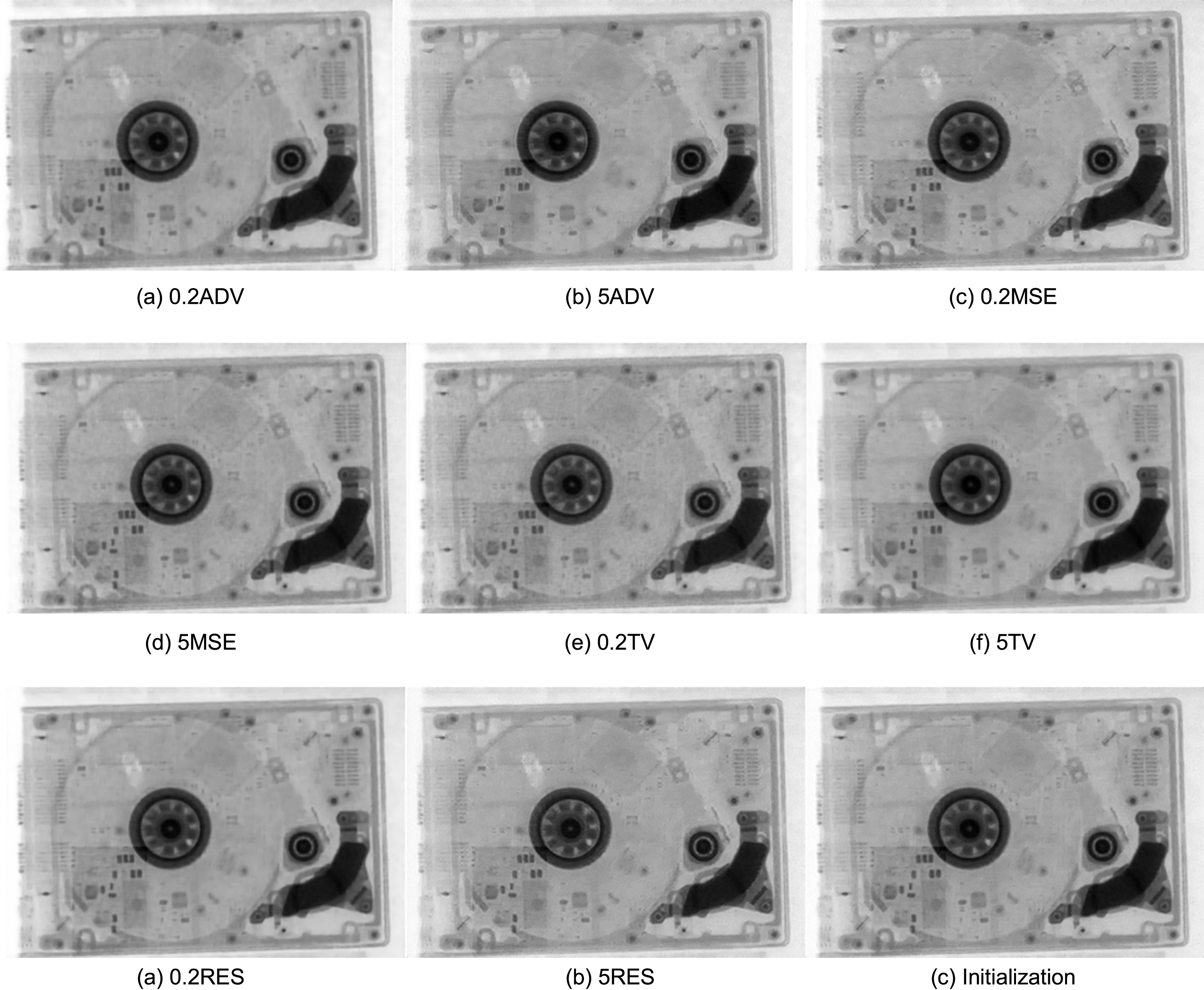
Table 2
Average PDR results of different weights
| Weight | 0.2 | 0.5 | 1 | 2 | 5 |
|---|---|---|---|---|---|
| MSE | 0.070 | 0.065 | 0.061 | 0.076 | 0.090 |
| ADV | 0.116 | 0.087 | 0.061 | 0.066 | 0.078 |
| Content | 0.097 | 0.069 | 0.061 | 0.057 | 0.054 |
| TV | 0.073 | 0.059 | 0.061 | 0.063 | 0.064 |
5Discussion
The main purpose of this paper is to present a perceptual loss function for deep-learning based method, which is used for digital image denoising. As described above, although the MSE loss based methods minimize the Euclidean distances between generated image and original image, it also smooths the edges and details of the original image. The introduction of the generative adversarial network is helpful to release this problem, in which a discriminator network is trained to distinguish the generated images from the original noise-free images. The output of the discriminator network can be used as an adversarial loss to force a generator network delivers images with high-frequency details. Although the images generated by adversarial loss based methods are more perceptual satisfying, the generated details are quite different from original images. The artifacts brought by adversarial loss can be suppressed by total variation loss while the original details are maintained. Moreover, high-level features of the digital images extracted by a pre-trained Resnet-34 model can be used as a more perceptual satisfying loss function compared with MSE loss.
Despite the proposed method delivers more perceptual satisfying results than traditional CNN-based method, there are some problems need to be addressed.
1) Some artifacts still can be observed in the generated images.
2) The perceptual loss in this work contains the MSE loss, which means it is still a supervised method.
6Conclusions
We proposed an end-to-end deep learning method named DNGAN to reduce the statistical noise of digital radiology images. The DNGAN is built on a perceptual function, which consist of MSE loss, adversarial loss, content less and total variation loss. Among them, the adversarial loss is learned by generative adversarial networks, which forces the generated images to be more perceptually convincing. We trained and evaluated the proposed method on a training dataset obtained by a real x-ray imaging system. As a result, the proposed method can effectively reduce the noise while keeping the details and edges of the images. Compared with the traditional CNN-based denoising methods, this method generated more realistic images, which shows the great potential of GAN for x-ray image processing.
Acknowledgments
This work is supported by the Science Foundation of Chinese Nuclear Industry (20154602098).
References
[1] | Elbakri I.A. and Fessler J.A. , Statistical image reconstruction for polyenergetic X-ray computed tomography, IEEE Transactions on Medical Imaging 21: (2) ((2002) ), 89–99. |
[2] | Zhao Y. , Wu Y. , Zuo Z. , Suo H. , Zhao S. and Zhang H. , CT pulmonary angiography using different noise index with iterative reconstruction algorithm and dual energy CT imaging using different body mass indices: Image quality and radiation dose, Journal of X-ray Science and Technology 25: (1) ((2017) ), 79–91. |
[3] | Arnold B.A. , Noise Analysis in Digital Radiography, Digital Radiography. Springer US, (1986) . |
[4] | Manduca A. , Yu L. , Trzasko J.D. et al. Projection space denoising with bilateral filtering and CT noise modeling for dose reduction in CT, Medical Physics 36: (11) ((2009) ), 4911. |
[5] | Wang J. , Li T. , Lu H. et al. Penalized weighted least-squares approach to sinogram noise reduction and image reconstruction for low-dose X-ray computed tomography, IEEE Transactions on Medical Imaging 25: (10) ((2006) ), 1272–1283. |
[6] | Xu Q. , Yu H. , Wang G. et al. Dictionary learning based low-dose X-ray CT reconstruction, Proceedings of SPIE – The International Society for Optical Engineering 9212: ((2014) ), 921207. |
[7] | Pisana F. , Henzler T. Schönberg, S et al. . Noise reduction and functional maps image quality improvement in dynamic CT perfusion using a new k-means clustering guided bilateral filter (KMGB), Medical Physics 44: (7) ((2017) ). |
[8] | Hu C. , Yi Z. , Zhang W. et al. Low-dose CT via convolutional neural network, Biomedical Optics Express 8: (2) ((2017) ), 679. |
[9] | Chen H. , Zhang Y. , Kalra M.K. et al. Low-dose CT with a Residual Encoder-Decoder Convolutional Neural Network (RED-CNN), arXiv preprint arXiv:1702.00288, (2017) . |
[10] | Kang E. , Ye J.C. et al. Wavelet domain residual network (wavresnet) for low-dose x-ray CT reconstruction, arXiv preprint arXiv: 1703.01383,(2017) . |
[11] | Wolterink J.M. , Leiner T. , Viergever M.A. et al. Generative adversarial networks for noise reduction in low-dose CT, IEEE Transactions on Medical Imaging PP: (99) ((2017) ), 1. |
[12] | Yang Q. , Yan P. , Zhang Y. et al. Low Dose CT Image Denoising Using a Generative Adversarial Network with Wasserstein Distance and Perceptual Loss, arXiv preprint arXiv: 1703.01383, (2017) . |
[13] | Goodfellow I.J. , Pouget-Abadie J. , Mirza M. et al. Generative adversarial nets, pp, International Conference on Neural Information Processing Systems MIT Press, (2014) , 2672–2680. |
[14] | Dabov K. , Foi A. , Katkovnik V. et al. Image denoising by sparse 3-D transform-domain collaborative filtering, IEEE Transactions on Image Processing 16: (8) ((2007) ), 2080. |
[15] | Gu S. , Zhang L. , Zuo W. et al. Weighted nuclear norm minimization with application to image denoising, computer vision and pattern recognition, IEEE ((2014) ), 2862–2869. |
[16] | He K. , Zhang X. , Ren S. et al. Spatial pyramid pooling in deep convolutional networks for visual recognition,&, Machine Intelligence 37: (9) ((2015) ), 1904. |
[17] | Zhang N. , Donahue J. , Girshick R. et al. Part-based R-CNNs for fine-grained category detection, 8689: ((2014) ), 834–849. |
[18] | Szegedy C. , Liu W. , Jia Y. , Sermanet P. , Reed S. , Anguelov D. , Erhan D. , Vanhoucke V. and Rabinovich A. , Going deeper with convolutions, pp, Proceedings of the IEEE Conference on Computer Vision and Pattern Recognition ((2015) ), 1–9. |
[19] | He K. , Zhang X. , Ren S. and Sun J. , Deep residual learning for image recognition, 2016 IEEE Conference on Computer Vision and Pattern Recognition (CVPR), (2016) . |
[20] | Denton E. , Chintala S. , Szlam A. and Fergus R. , Deep generative image models using a laplacian pyramid of adversarial networks. In pp, Advances in Neural Information Processing Systems (NIPS) ((2015) ), 1486–1494. |
[21] | Li C. and Wand M. , Combining Markov Random Fields and Convolutional Neural Networks for Image Synthesis. In pp, IEEE Conference on Computer Vision and Pattern Recognition (CVPR) ((2016) ), 2479–2486. |
[22] | Ledig C. , Theis L. , Huszar F. et al. Photo-Realistic Single Image Super-Resolution Using a Generative Adversarial Network, arXiv preprint arXiv:1609.04802, (2016) . |
[23] | Ignatov A. , Kobyshev N. , Vanhoey K. , et al. DSLR-Quality Photos on Mobile Devices with Deep Convolutional Networks, arXiv preprint arXiv:1704.02470, (2017) . |
[24] | Simonyan K. and Zisserman A. , Very deep convolutional networks for large-scale image recognition, Computer Science ((2014) ). |
[25] | Kim J. , Kwon J. Lee and K. Mu Lee, Accurate image super-resolution using very deep convolutional networks, Proceedings of the IEEE Conference on Computer Vision and Pattern Recognition ((2016) ), 1646–1654. |
[26] | Dong C. , Loy C.C. , He K. and Tang X. , Image super-resolution using deep convolutional networks, IEEE Transactions on Pattern Analysis & Machine Intelligence 38: (2) ((2015) ), 295–307. |
[27] | Kingma D. and Ba J. , Adam: A method for stochastic optimization, arXiv preprint arXiv:1412.6980, (2014) . |
[28] | Zhang R. , Isola P. , Efros A.A. , Shechtman E. and Wang O. , The unreasonable effectiveness of deep networks as a perceptual metric, in: CVPR, (2018) . |


