
Bounding the return on investment and projecting the costs of expanding PROMISE services and activities: Initial insights from PROMISE for policymakers
Abstract
BACKGROUND:
Promoting Readiness of Minors in SSI (PROMISE) is a uniquely large initiative, with over $229 million awarded to sites across the country, by the U.S. Departments of Education, Labor, and Health and Human services to improve the education and employment outcomes for youth who receive Supplemental Security Income (SSI) and their families.
OBJECTIVE:
Policy makers need a clear understanding of the impact of the PROMISE intervention and the cost to roll out policy changes to the broader population; however, a comprehensive return on investment (ROI) analysis of PROMISE will not be available for many years, as it will require long-run information on the employment patterns of the participants. Although a full ROI analysis will be an essential tool to evaluate the policy implications of PROMISE, there is also a current need to understand the range of the ROI. To that end, this study aims to frame the bounds of the ROI for PROMISE and highlight the costs of expanding the availability of select services.
CONCLUSION:
The bounds of the ROI are determined by estimating the range of lifetime cost savings over levels of employment for SSI youth, accounting for benefit receipt and tax revenue. Using administrative data from the PROMISE sites, the study additionally estimates the cost to expanding select PROMISE services or activities within each state or site.
1Introduction
The PROMISE initiative represented a significant effort to address the poor transition outcomes of SSI youth. The PROMISE intervention model was jointly developed by the US Department of Education, the Social Security Administration (SSA), the U.S. Department of Health and Human Services, and the U.S. Department of Labor. The Consolidated Appropriations Act, 2012 (P.L. 112-74) provided funds for activities to six model demonstration projects across the country: Arkansas, California, Maryland, New York, Wisconsin, and a consortium of states (Arizona, Colorado, Montana, North Dakota, South Dakota, and Utah). Additionally, a PROMISE Technical Assistance Center was awarded to the Association of University Centers on Disabilities in 2014. Overall, the projects received a total of approximately $229 million for the five-year intervention.
The PROMISE model aimed to improve the outcomes of child SSI recipients and their families by targeting four key areas: interagency partnerships, services and supports, participant recruitment and outreach, and technical assistance. Sites were tasked to develop and strengthen interagency partnerships within their states. The constellation of these agencies varied by site, but the required partners provided vocational rehabilitation (VR) services, special education services, workforce development services, Medicaid services, developmental and intellectual disabilities services, mental health services, and Temporary Assistance for Needy Families services. Another core element was the expanded provision of services and supports, including case management, work-based learning experiences, parent/guardian training, and benefits counseling and financial literacy training. Sites engaged in regular, monitored outreach and recruitment with the participants. Finally, all sites provided technical assistance and training that supported professional development of the relevant stakeholders within their state.
The PROMISE intervention attempted to change multiple policy-relevant factors that when taken together lead to poor outcomes for child SSI recipients as they transition from high school. Policy makers need a clear understanding of the impact of the PROMISE intervention and the cost to roll out policy changes to the broader population. A comprehensive return on investment (ROI) analysis will not be possible for many years in the future. Once the PROMISE youth have had the opportunity to establish an employment pattern, estimation models can be used to determine the predicted ROI. While a full ROI report will be an essential tool to evaluate the policy implications of PROMISE, there is also a current need to understand the range of the ROI. To that end, this report identifies the upper bound of potential cost savings of a program like PROMISE.
The purpose of this study is to frame the bounds of the return on investment for PROMISE and highlight the costs of expanding the availability of select services. The analysis integrates data from multiple sources to generate measures of total lifetime SSI and Medicaid receipt for SSI youth. The estimates were allowed to vary by sex and labor market attachment. Models also accounted for tax revenue from earnings.
2Youth SSI population
Nearly 1.2 million individuals under the age of 18 received SSI benefits in 2017. This represents a 39.7% increase in the SSI rolls for youth since 2000 (Social Security Administration, 2017). This population of youth are ones who rarely leave the SSA rolls (Hemmeter, Kauff & Wittenburg, 2009; Hemmeter & Gilby, 2009), have low educational and employment attainment, rarely participate in vocational rehabilitation (Martinez et al., 2010), experience higher rates of incarceration (Quinn, Rutherford, Leone, Osher & Poirier, 2005) and higher school dropout rates, and often do not have access to transition support services (Hemmeter, Kauff, & Wittenburg, 2009).
Currently youth in SSI account for one in every seven SSI recipients, with approximately $9.2 billion in total annual payments including federally administrated state supplements (Social Security Administration, 2017). When these youth reach age 18, they must have their eligibility redetermined using the definition of disability for adults. Over half are initially redetermined as eligible and an additional eighth are successful in appealing the initial cessation or thereafter reapplying (Hemmeter & Gilby, 2009). With the rapidly growing adult SSI roles and only 4.8% of the adult SSI population working (Social Security Administration, 2017), there is a clear need for policy makers to have an understanding of the potential return on investment for interventions like PROMISE.
3Method
To participate in PROMISE, youth needed to be receiving SSI due to a disability and be between 14 and 16 years old. Additionally, youth had to live in one of the participating states, and sometimes in specific cities in the state, to be eligible to participate in the study. The states included Arizona, Arkansas, California, Colorado, Maryland, Montana, New York, North Dakota, South Dakota, Utah, and Wisconsin.
While PROMISE youth certainly received other forms of government assistance and welfare support, this analysis focuses on SSI and Medicaid costs. Specifically, this analysis posed this question:
What is the cost in continued SSI benefits and Medicaid costs across a lifetime for four potential scenarios for the PROMISE youth: (1) an individual who never joins the workforce, (2) an individual with limited employment, (3) an individual employed part-time in a minimum-wage job, and (4) an individual employed full-time in a minimum-wage job?
As income increases, SSI benefits decrease and Medicaid eligibility decreases while tax revenue increases. The model allows Medicaid eligibility to change with income level. While the model allows SSI benefit amount to change in income level, it assumes SSI eligibility across the four scenarios. The no employment and limited employment options are designed scenarios where the individual is eligible for SSI. Following Deshpande (2016), the part-time employment option represents individuals who do not maintain SSI eligibility at the age 18 redetermination. The full-time employment scenario also assumes the individual is ineligible for SSI. Table 1 shows the elements that contribute to the ROI estimation.
Table 1
Expected SSI benefits, Medicaid costs, and paid taxes by employment type in adulthood
| Employment Type in Adulthood | SSI Benefits | Medicaid Costs | Taxes Paid |
| No employment | Yes | Yes | No |
| Limited employment | Yes | Yes | Yes |
| Part-time employment | No | Yes | Yes |
| Full-time employment | No | Varies | Yes |
3.1Life expectancy
Although multiple sources were available for life expectancy, few studies explicitly took disability into account (Chetty et al., 2016; Kegler, Baldwin, Rudd, & Walsh, 2017; Sasson, 2016). Those that did do so discussed how many years of life before the expected start of a disabling health condition (Crimmins, Zhang, & Saito, 2016; Laditka & Laditka, 2016). Two sources included in this analysis were based on actuarial data from the SSA Office of the Chief Actuary, one for the general population (Bell and Miller, 2005) and one for individuals age 26 who had lived 10 or more years with a disability (Zayatz, 2005). A third source of life expectancy estimates for the analysis were based on results from the Wisconsin Longitudinal Study (WLS), which explicitly accounted for disability in life expectancy estimates (Ng, Shaw & Peeters, 2018). The WLS estimates are based on a sample who lived to age 60, so these estimates skewed toward a higher average. All three sources provided life expectancy estimates by sex. Glei and Horiuchi (2007) point to the gap in life expectancy that started in the early 1900’s, reconfirmed in their analysis that covered mortality rates from 1751 to 2004 across 29 countries. The life expectancy estimates from these three sources broken out by sex is shown in Figure 1.
Fig.1
Life expectancy for people in the general population and those with disabilities. General Population estimates from 2014 and With Disabilities 1996-2000 are based on actuarial estimates from the Social Security Administration. The Wisconsin Longitudinal Study data was collected from 1957–2011.
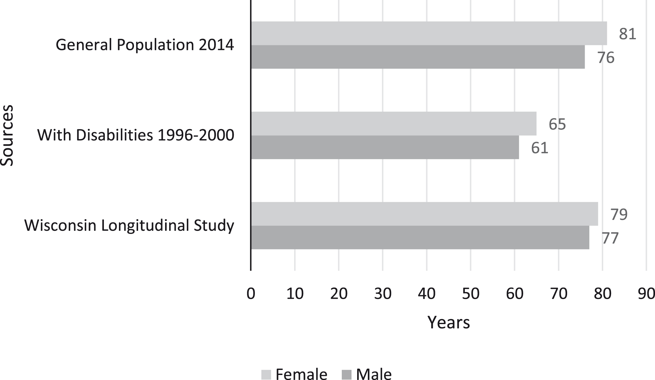
As one would expect, the life expectancy for the general population, which includes people with and without disabilities, contains the highest values for life expectancy when compared descriptively to the other two sources (Bell & Miller, 2005). Approximately 12.7% of the general population (Erickson, Lee, & von Schrader, 2017) has a disability, so those individuals with disabilities are represented in this sample. The impact of disability on life expectancy is unclear.
The lowest life expectancy estimates were based on data collected from 1996 to 2000 (SSA, 2005), approximately 20 years old at the time of this analysis. These estimates were based on someone age 26 who had lived 10 or more years with a disability, a scenario that matches PROMISE youth life experience, as they were only eligible for recruitment before their 17th birthday. As a point of comparison to the 1996 to 2000 SSA estimates (and not shown in Figure 1), the general population life expectancy in 2000 was 79.5 years for females and 74.1 years for males (Centers for Disease Control, 2002). The drawbacks of using older life expectancy estimates may be little (GBD 2015 DALYs and HALE Collaborators, 2016), but the difference between these disability-based estimates and general population estimates is 19.7% fewer years for those with disabilities.
A third source, the WLS, returned estimates from data collected as late as 2011 that included disability status (Ng et al., 2018). Unfortunately, Ng and colleagues (2018) did not distinguish between disability from childhood and disability acquired as an adult, but they provided estimates in years of how life expectancy was impacted for those with a disability, which resulted in life expectancy for women at 79.4 years and for men at 76.6 years. The WLS male life expectancy is higher than the general population estimate because the WLS sample excluded individuals who died before age 60. Conditional on living to age 60, the male-female life expectancy gap decreases but still exists in the WLS. That said, estimates from all three sources aligned with results for males with intellectual disability in Westphalia-Lippe, Germany, although males with intellectual disability in Baden-Wuerttemberg lived on average 65.3 years. A similar pattern as shown in Figure 1 was observed – females experience lower life expectancy than the general population but higher than males (Dieckmann, Giovis & Offergeld, 2015).
Aside from the WLS (Ng et al., 2018) that examined people with disabilities as a single group, most other research has focused on specific disability statuses like intellectual disability (Dieckman et al., 2015), cerebral palsy (Brooks et al., 2014), and traumatic brain injury (Harrison-Felix, et al., 2012). In the WLS, other factors such as smoking and obesity were also included. For the estimate of the upper bound of lifetime SSI and Medicaid receipt, three values were calculated for each for the six life expectancy estimates shown in Figure 1.
3.2SSI and Medicaid costs
The ROI analysis requires estimates of the present discounted value of the stream of SSI benefits and Medicaid costs. The starting value for SSI was $8,520, based on 2013 SSI payment amounts (Social Security Administration, 2019a). The expected annual SSI increase was 3.0%, the median historical cost-of-living adjustment made to SSI by SSA (Social Security Administration, 2019b). The initial value for annual Medicaid cost, $16,859, was based on 2014 estimates for individuals with disabilities (Kaiser Family Foundation, 2014). Projections for growth in Medicaid spending, 3.6% annually, were based on numbers from the Medicaid and CHIP Payment and Access Commission (2016). All calculations started at age 18 and each year’s expenditures are based on the previous year’s value multiplied by one plus the increase and then discounted to present dollars using a 2.0% inflation rate (Federal Open Market Committee, 2019). This formula was applied across the years until the final life expectancy year, rounded to the whole year shown in Figure 1, and then summed across the life span.
3.4Upper bound of lifetime benefit receipt
ROI estimates were built starting at age 18 through the average life expectancy by sex. Three life expectancy values were used: general population based on 2014 life tables, 1996–2000 estimates, and WLS. The results from those calculations, listed in Table 2, provided the expected individual total lifetime receipt of SSI, total lifetime Medicaid expenditures, and the sum of those values. These totals could be as high as $2.3 million for males and $2.6 million for females if 2014 general population estimates are used, estimates that by definition include individuals with and without disabilities. If individuals with disabilities live on average as long as the general population and the annual increase remains approximately the same, these are the amounts that could be paid out over 59–64 years to individuals with disabilities who never enter the workforce. If the life expectancy is shortened by 19.7% to match the 1996–2000 estimates, the lifetime cost would be 1.5 million for men and $1.7 million for women. The 1996–2000 life expectancy estimates are the most relevant to this population as they account for disability and do not presume that the population lives until age 60.
Table 2
Total expected lifetime benefits in dollars for an individual by program and sex
| Life expectancy estimates | SSI | Medicaid | Total |
| Male | |||
| General Population from 2014 | 676,307 | 1,617,563 | 2,293,870 |
| 1996–2000 Estimates | 465,926 | 1,056,976 | 1,522,902 |
| Wisconsin Longitudinal Study | 691,457 | 1,659,796 | 2,351,253 |
| Female | |||
| General Population from 2014 | 753,559 | 1,835,456 | 2,589,014 |
| 1996–2000 Estimates | 519,052 | 1,193,912 | 1,712,965 |
| Wisconsin Longitudinal Study | 722,205 | 1,746,259 | 2,468,464 |
Note: Estimates of the upper bound of lifetime SSI and Medicaid benefit receipt by sex and life expectancy. Dollar values adjusted for inflation.
These values provide the upper bound of program costs for each person under the most extreme scenario where a youth on SSI never enters the workforce. Given the total expenditure of $229 million to implement PROMISE to 13,444 youth, these estimates indicate that an equivalent amount would have been spent in SSI benefits and Medicaid costs for between 17 and 25 males or 15 and 22 females who never engage in paid work.
3.5Labor market attachment
Beyond working-aged SSI recipients, individuals with disabilities in the United States face poorer labor market outcomes than their peers without disabilities. Only 37.3% of working-aged individuals with disabilities are employed compared to 79.4% of those without disabilities. When they do work, they are employed less intensively, 23.9% versus 60.3% working full-time and full-year. Consequently, working-aged individuals with disabilities face higher rates of poverty, 26.1% compared to 10.4% (Erickson, Lee, & von Schrader, 2017). Hence, individuals with disabilities no longer receiving SSI benefits are reasonably modeled under the scenarios of part-time and full-time employment at minimum wage.
The fact that SSI eligibility has income restrictions implies that the observed labor market attachment of SSI recipients will be weaker than the general population. Among working-aged SSI recipients in 2017, only 4.8% engaged in paid work (SSI ASR, 2017). Looking at the employment patterns of adult SSI recipients in the five years prior to benefit receipt reveals that roughly a quarter of them were employed in each year (Daly, 1998). Thus, the two modeled scenarios, no and limited workforce participation, for individuals still receiving SSI benefits align with the evidence for this population.
3.6Tax revenue
Expected taxes paid were obtained from TAXSIM, tax simulation software that utilizes federal and state tax law information by state to generate estimates of expected tax liability (Feenberg & Coutts, 1993). Tax estimates were obtained for Arizona, Arkansas, California, Colorado, Maryland, Montana, New York, North Dakota, South Dakota, Utah, and Wisconsin, the states involved in PROMISE. Tax estimates assumed offsetting income growth and inflation and did not assume any increase in income or change in future tax rates, resulting in conservative estimates of an individual’s tax liability across a lifetime. Paid taxes did assume that the person started working and paying taxes at age 18. To remain conservative in the estimation of the lower bound, the lowest life expectancies were selected.
Tax estimates, unchanging across the lifetime, were obtained for three levels of employment. Prior evidence shows that youth on SSI who continue on SSI after the age 18 redetermination earn $1,500 annually while those determined ineligible at 18 earn $4,720 annually, both adjusted to 2018 dollars (Deshpande, 2016). The former group are represented under the limited employment label in Table 1 while the latter are represented by the part-time label. An individual employed at minimum wage would earn these amounts by working roughly 3 and 10 hours per week, respectively. The part-time group is modeled under the assumption that they did not maintain SSI eligibility following the age 18 redetermination, which aligns with the evidence in Deshpande (2016). The final group considered in this paper is those employed full-time, full-year in a minimum-wage position, and like the tax estimates, the income estimates did not change over time.
Due to variation in the minimum wage across the PROMISE states, the annual earnings for the full-time group range between $15,080 and $23,088, as seen in Table 3. States also vary in their income eligibility requirements for Medicaid. Income relative to the federal poverty level and number of dependents are key determinants of Medicaid eligibility. Table 3 shows how the projected earnings level and four different household scenarios correspond to Medicaid eligibility in each state.
Table 3
Projected annual earnings and Medicaid eligibility among full-time employment group, by marital status and number of dependents
| State | Earnings ($) | Single, no dependents | Single, dependents | Married, no dependents | Married, dependents |
| Arizona | 22,880 | No | No | No | Yes |
| Arkansas | 19,240 | No | Yes | Yes | Yes |
| California | 22,880 | No | Yes | Yes | Yes |
| Colorado | 22,880 | No | No | No | Yes |
| Maryland | 21,008 | No | Yes | Yes | Yes |
| Montana | 17,680 | No | Yes | Yes | Yes |
| New York | 23,088 | No | Yes | Yes | Yes |
| North Dakota | 15,080 | Yes | Yes | Yes | Yes |
| South Dakota | 18,928 | Yes | Yes | Yes | Yes |
| Utah | 15,080 | Yes | Yes | Yes | Yes |
| Wisconsin | 15,080 | No | Yes | Yes | Yes |
Note: Earnings estimated as the product of 52 weeks worked at 40 hours per week for the state-specific minimum wage.
For three levels of employment, TAXSIM accounted for a set of essential input variables. Estimates were prepared of each of the 11 PROMISE states, the three levels of employment described above, and estimated gross social security benefit. Only individuals with limited employment were assumed to remain in SSI. Marital status was allowed to vary. The number of dependents ranged between zero and one, which is representative of the SSI receiving population –70.8% have no children and 14.4% have one child (Stegman & Hemmeter, 2014).
3.7Lower bound of lifetime benefit receipt
For the individual with a disability who never enters the workforce, we calculated expected lifetime receipt of SSI and Medicaid expenditures as shown in Table 2. We now consider three alternate scenarios where individuals engage in different levels of paid work. For these employed individuals, money flows back into the system in forms of federal tax liability, state tax liability, and the U.S. federal payroll tax referred as FICA. For each state that was part of PROMISE, estimated tax liabilities and FICA payments were summed and then multiplied by the expected working life by sex, i.e., 44 years for men and 48 years for women. The resulting lifetime estimates of tax liability and FICA payments are reported in Table 4.
Table 4
Total tax and FICA lifetime payments in dollars for an individual by sex, marital status, dependent status, state, and employment level
| Male | Female | |||||
| Limited | Part-Time | Full-Time | Limited | Part-Time | Full-Time | |
| Arizona | ||||||
| Single, no dependents | 3,949 | 14,788 | 234,894 | 4,308 | 16,132 | 256,248 |
| Single, dependents | 2,849 | 13,688 | 182,985 | 3,108 | 14,932 | 199,620 |
| Married, no dependents | 2,849 | 13,688 | 171,086 | 3,108 | 14,932 | 186,639 |
| Married, dependents | 1,749 | 12,588 | 155,380 | 1,908 | 13,732 | 169,505 |
| Arkansas | ||||||
| Single, no dependents | 5,049 | 15,888 | 188,320 | 5,508 | 17,332 | 205,440 |
| Single, dependents | 5,049 | 15,888 | 149,155 | 5,508 | 17,332 | 162,715 |
| Married, no dependents | 5,049 | 15,888 | 125,503 | 5,508 | 17,332 | 136,913 |
| Married, dependents | 5,049 | 15,888 | 125,503 | 5,508 | 17,332 | 136,913 |
| California | ||||||
| Single, no dependents | 785 | 10,208 | 224,412 | 857 | 11,136 | 244,813 |
| Single, dependents | 785 | 10,208 | 178,140 | 857 | 11,136 | 194,335 |
| Married, no dependents | 785 | 10,208 | 163,620 | 857 | 11,136 | 178,495 |
| Married, dependents | 785 | 10,208 | 154,028 | 857 | 11,136 | 168,031 |
| Colorado | ||||||
| Single, no dependents | 4,544 | 14,299 | 241,847 | 4,957 | 15,599 | 263,833 |
| Single, dependents | 4,544 | 14,299 | 189,304 | 4,957 | 15,599 | 206,513 |
| Married, no dependents | 4,544 | 14,299 | 168,061 | 4,957 | 15,599 | 183,339 |
| Married, dependents | 4,544 | 14,299 | 154,028 | 4,957 | 15,599 | 168,031 |
| Maryland | ||||||
| Single, no dependents | 3,736 | 11,774 | 222,092 | 4,076 | 12,845 | 242,282 |
| Single, dependents | 3,736 | 11,757 | 178,936 | 4,076 | 12,826 | 195,203 |
| Married, no dependents | 3,736 | 11,757 | 164,416 | 4,076 | 12,826 | 179,363 |
| Married, dependents | 3,736 | 11,757 | 156,372 | 4,076 | 12,826 | 170,588 |
| Montana | ||||||
| Single, no dependents | 5,049 | 16,046 | 165,583 | 5,508 | 17,505 | 180,636 |
| Single, dependents | 5,049 | 15,888 | 129,071 | 5,508 | 17,332 | 140,805 |
| Married, no dependents | 5,049 | 15,888 | 118,568 | 5,508 | 17,332 | 129,347 |
| Married, dependents | 5,049 | 15,888 | 114,916 | 5,508 | 17,332 | 125,363 |
| New York | ||||||
| Single, no dependents | 3,535 | 11,121 | 246,928 | 3,856 | 12,132 | 269,376 |
| Single, dependents | (866) | 6,721 | 192,302 | (945) | 7,332 | 209,784 |
| Married, no dependents | 3,535 | 11,121 | 175,494 | 3,856 | 12,132 | 191,448 |
| Married, dependents | (866) | 6,721 | 158,302 | (945) | 7,332 | 172,693 |
| North Dakota | ||||||
| Single, no dependents | 5,049 | 15,888 | 124,620 | 5,508 | 17,332 | 135,949 |
| Single, dependents | 5,049 | 15,888 | 101,519 | 5,508 | 17,332 | 110,748 |
| Married, no dependents | 5,049 | 15,888 | 83,496 | 5,508 | 17,332 | 91,086 |
| Married, dependents | 5,049 | 15,888 | 83,496 | 5,508 | 17,332 | 91,086 |
| South Dakota | ||||||
| Single, no dependents | 5,049 | 15,888 | 165,166 | 5,508 | 17,332 | 180,181 |
| Single, dependents | 5,049 | 15,888 | 134,146 | 5,508 | 17,332 | 146,341 |
| Married, no dependents | 5,049 | 15,888 | 122,353 | 5,508 | 17,332 | 133,476 |
| Married, dependents | 5,049 | 15,888 | 122,353 | 5,508 | 17,332 | 133,476 |
| Utah | ||||||
| Single, no dependents | 5,049 | 15,888 | 131,549 | 5,508 | 17,332 | 143,508 |
| Single, dependents | 5,049 | 15,888 | 101,519 | 5,508 | 17,332 | 110,748 |
| Married, no dependents | 5,049 | 15,888 | 83,496 | 5,508 | 17,332 | 91,086 |
| Married, dependents | 5,049 | 15,888 | 83,496 | 5,508 | 17,332 | 91,086 |
| Wisconsin | ||||||
| Single, no dependents | 5,049 | 15,888 | 129,586 | 5,508 | 17,332 | 141,366 |
| Single, dependents | 4,847 | 15,252 | 102,291 | 5,288 | 16,639 | 111,590 |
| Married, no dependents | 5,049 | 15,888 | 83,496 | 5,508 | 17,332 | 91,086 |
| Married, dependents | 4,847 | 15,252 | 82,775 | 5,288 | 16,639 | 90,300 |
Notes: Estimates of lifetime tax and FICA payment by sex, marital status, dependent status, state, and employment level. Projected values account for 44 working years by men and 48 years by women. Negative values shown in parentheses.
Across all states, the tax liabilities were non-positive values for the limited and part-time employment levels, but with FICA added to tax liabilities the lifetime totals were all positive except for people with dependents working under limited employment in New York. Unsurprisingly, the limited employment scenario, which earns only $1,500 annually, yields little back into the government in terms of direct revenue. Individuals modeled working full-time at minimum wage are expected to generate tax revenue between $82,775 and $269,376 across their lifetimes.
The estimate of the lower bound for the ROI offsets SSI and Medicaid costs against tax revenue. Table 5 reports this offset amount for each of the three employment levels and by sex and state. For those individuals receiving SSI with limited employment, the amount paid in taxes and FICA is minimal relative to the amount received from SSI and Medicaid. Therefore, the lower bound of benefits does not differ much from the upper bound of benefits, ranging between $1.5 million and $1.7 million. Individuals with part-time employment receive a net $1.0 million to $1.2 million in benefits, which represents a reduction in lifetime benefits by approximately a third. The full-time employment scenario varies considerably by state and household structure from net benefit receipt of $1.1 million to net revenue of $269,376. For example, a single female living in Arizona with no dependents would receive $1.7 million in benefits over the course of her life under limited employment but would net contribute $256,248 back in tax revenue under a full-time employment scenario. This alternative employment path represents a $2.0 million benefit to the government.
Table 5
Total expected lifetime benefits in dollars for an individual by sex, marital status, dependent status, state, and employment level
| Male | Female | |||||
| Limited | Part-Time | Full-Time | Limited | Part-Time | Full-Time | |
| Arizona | ||||||
| Single, no dependents | 1,505,828 | 1,042,188 | (234,894) | 1,694,035 | 1,193,912 | (256,248) |
| Single, dependents | 1,506,928 | 1,043,288 | (182,985) | 1,695,235 | 1,178,980 | (199,620) |
| Married, no dependents | 1,506,928 | 1,043,288 | (171,086) | 1,695,235 | 1,178,980 | (186,639) |
| Married, dependents | 1,508,028 | 1,044,388 | 901,596 | 1,696,435 | 1,180,180 | 1,024,407 |
| Arkansas | ||||||
| Single, no dependents | 1,504,728 | 1,041,088 | (188,320) | 1,692,835 | 1,176,580 | (205,440) |
| Single, dependents | 1,504,728 | 1,041,088 | 907,821 | 1,692,835 | 1,176,580 | 1,031,197 |
| Married, no dependents | 1,504,728 | 1,041,088 | 931,473 | 1,692,835 | 1,176,580 | 1,056,999 |
| Married, dependents | 1,504,728 | 1,041,088 | 931,473 | 1,692,835 | 1,176,580 | 1,056,999 |
| California | ||||||
| Single, no dependents | 1,508,992 | 1,046,768 | (224,412) | 1,697,486 | 1,182,776 | (244,813) |
| Single, dependents | 1,508,992 | 1,046,768 | 878,836 | 1,697,486 | 1,182,776 | 999,577 |
| Married, no dependents | 1,508,992 | 1,046,768 | 893,356 | 1,697,486 | 1,182,776 | 1,015,417 |
| Married, dependents | 1,508,992 | 1,046,768 | 902,948 | 1,697,486 | 1,182,776 | 1,025,881 |
| Colorado | ||||||
| Single, no dependents | 1,505,233 | 1,042,677 | (241,847) | 1,693,386 | 1,178,313 | (263,833) |
| Single, dependents | 1,505,233 | 1,042,677 | (189,304) | 1,693,386 | 1,178,313 | (206,513) |
| Married, no dependents | 1,505,233 | 1,042,677 | (168,061) | 1,693,386 | 1,178,313 | (183,339) |
| Married, dependents | 1,505,233 | 1,042,677 | 902,948 | 1,693,386 | 1,178,313 | 1,025,881 |
| Maryland | ||||||
| Single, no dependents | 1,506,041 | 1,045,202 | (222,092) | 1,694,267 | 1,181,067 | (242,282) |
| Single, dependents | 1,506,041 | 1,045,219 | 878,040 | 1,694,267 | 1,181,086 | 998,709 |
| Married, no dependents | 1,506,041 | 1,045,219 | 892,560 | 1,694,267 | 1,181,086 | 1,014,549 |
| Married, dependents | 1,506,041 | 1,045,219 | 900,604 | 1,694,267 | 1,181,086 | 1,023,324 |
| Montana | ||||||
| Single, no dependents | 1,504,728 | 1,040,930 | (165,583) | 1,692,835 | 1,176,407 | (180,636) |
| Single, dependents | 1,504,728 | 1,041,088 | 927,905 | 1,692,835 | 1,176,580 | 1,053,107 |
| Married, no dependents | 1,504,728 | 1,041,088 | 938,408 | 1,692,835 | 1,176,580 | 1,064,565 |
| Married, dependents | 1,504,728 | 1,041,088 | 942,060 | 1,692,835 | 1,176,580 | 1,068,549 |
| New York | ||||||
| Single, no dependents | 1,506,242 | 1,045,855 | (246,928) | 1,694,487 | 1,181,780 | (269,376) |
| Single, dependents | 1,510,643 | 1,050,255 | 864,674 | 1,699,288 | 1,186,580 | 984,128 |
| Married, no dependents | 1,506,242 | 1,045,855 | 881,482 | 1,694,487 | 1,181,780 | 1,002,464 |
| Married, dependents | 1,510,643 | 1,050,255 | 898,674 | 1,699,288 | 1,186,580 | 1,021,219 |
| North Dakota | ||||||
| Single, no dependents | 1,504,728 | 1,041,088 | 932,356 | 1,692,835 | 1,176,580 | 1,057,963 |
| Single, dependents | 1,504,728 | 1,041,088 | 955,457 | 1,692,835 | 1,176,580 | 1,083,164 |
| Married, no dependents | 1,504,728 | 1,041,088 | 973,480 | 1,692,835 | 1,176,580 | 1,102,826 |
| Married, dependents | 1,504,728 | 1,041,088 | 973,480 | 1,692,835 | 1,176,580 | 1,102,826 |
| South Dakota | ||||||
| Single, no dependents | 1,504,728 | 1,041,088 | 891,810 | 1,692,835 | 1,176,580 | 1,013,731 |
| Single, dependents | 1,504,728 | 1,041,088 | 922,830 | 1,692,835 | 1,176,580 | 1,047,571 |
| Married, no dependents | 1,504,728 | 1,041,088 | 934,623 | 1,692,835 | 1,176,580 | 1,060,436 |
| Married, dependents | 1,504,728 | 1,041,088 | 934,623 | 1,692,835 | 1,176,580 | 1,060,436 |
| Utah | ||||||
| Single, no dependents | 1,504,728 | 1,041,088 | 925,427 | 1,692,835 | 1,176,580 | 1,050,404 |
| Single, dependents | 1,504,728 | 1,041,088 | 955,457 | 1,692,835 | 1,176,580 | 1,083,164 |
| Married, no dependents | 1,504,728 | 1,041,088 | 973,480 | 1,692,835 | 1,176,580 | 1,102,826 |
| Married, dependents | 1,504,728 | 1,041,088 | 973,480 | 1,692,835 | 1,176,580 | 1,102,826 |
| Wisconsin | ||||||
| Single, no dependents | 1,504,728 | 1,041,088 | (129,586) | 1,692,835 | 1,176,580 | (141,366) |
| Single, dependents | 1,504,930 | 1,041,724 | 954,685 | 1,693,055 | 1,177,273 | 1,082,322 |
| Married, no dependents | 1,504,728 | 1,041,088 | 973,480 | 1,692,835 | 1,176,580 | 1,102,826 |
| Married, dependents | 1,504,930 | 1,041,724 | 974,201 | 1,693,055 | 1,177,273 | 1,103,612 |
Notes: Estimates of lifetime SSI benefits and Medicaid costs net any tax and FICA payment by sex, marital status, dependent status, state, and employment level. Projected values account for 44 working years by men and 48 years by women. Negative values shown in parentheses.
The PROMISE intervention aimed to improve the employment outcomes for youth on SSI. This analysis has examined the lifetime net benefit receipt for three different employment outcomes with increasing attachment to the labor market. Table 6 reports, by state, the number of youth in that state who would need to work over their lifetime to offset the $229 million spent nationally on PROMISE. These numbers are not based on the recruited PROMISE population but rather are a function of the cost of PROMISE relative to the reduction in benefits and increase in tax revenue resulting from increased earnings. Both part-time and full-time employment have the ability to substantially offset the cost of the project. On average, 477 youth, i.e., a number equivalent to 7.1% of the roughly 6,700 intervention youth, would need to move from never working to part-time employment to completely cover the cost of PROMISE. In other words, 477 of the intervention youth being employed part-time over their entire working lives would cumulatively offset the cost of PROMISE through reductions in benefit receipt and increases in tax revenue. As Table 6 shows, the benefit of work is so significant that in New York only 129 male youth working full-time over their lives (assuming they also are single with no dependents) could cover the full cost of the national PROMISE initiative.
Table 6
Number of youth needed to offset cost of PROMISE by sex, marital status, dependent status, state, and employment level
| Male | Female | |||||
| Limited | Part-Time | Full-Time | Limited | Part-Time | Full-Time | |
| Arizona | ||||||
| Single, no dependents | 13,412 | 476 | 130 | 12,097 | 441 | 116 |
| Single, dependents | 14,336 | 477 | 134 | 12,916 | 429 | 120 |
| Married, no dependents | 14,336 | 477 | 135 | 12,916 | 429 | 121 |
| Married, dependents | 15,396 | 479 | 369 | 13,854 | 430 | 333 |
| Arkansas | ||||||
| Single, no dependents | 12,600 | 475 | 134 | 11,376 | 427 | 119 |
| Single, dependents | 12,600 | 475 | 372 | 11,376 | 427 | 336 |
| Married, no dependents | 12,600 | 475 | 387 | 11,376 | 427 | 349 |
| Married, dependents | 12,600 | 475 | 387 | 11,376 | 427 | 349 |
| California | ||||||
| Single, no dependents | 16,463 | 481 | 131 | 14,795 | 432 | 117 |
| Single, dependents | 16,463 | 481 | 356 | 14,795 | 432 | 321 |
| Married, no dependents | 16,463 | 481 | 364 | 14,795 | 432 | 328 |
| Married, dependents | 16,463 | 481 | 369 | 14,795 | 432 | 333 |
| Colorado | ||||||
| Single, no dependents | 12,961 | 477 | 130 | 11,696 | 428 | 116 |
| Single, dependents | 12,961 | 477 | 134 | 11,696 | 428 | 119 |
| Married, no dependents | 12,961 | 477 | 135 | 11,696 | 428 | 121 |
| Married, dependents | 12,961 | 477 | 369 | 11,696 | 428 | 333 |
| Maryland | ||||||
| Single, no dependents | 13,582 | 479 | 131 | 12,248 | 431 | 117 |
| Single, dependents | 13,582 | 479 | 355 | 12,248 | 431 | 321 |
| Married, no dependents | 13,582 | 479 | 363 | 12,248 | 431 | 328 |
| Married, dependents | 13,582 | 479 | 368 | 12,248 | 431 | 332 |
| Montana | ||||||
| Single, no dependents | 12,600 | 475 | 136 | 11,376 | 427 | 121 |
| Single, dependents | 12,600 | 475 | 385 | 11,376 | 427 | 347 |
| Married, no dependents | 12,600 | 475 | 392 | 11,376 | 427 | 353 |
| Married, dependents | 12,600 | 475 | 394 | 11,376 | 427 | 355 |
| New York | ||||||
| Single, no dependents | 13,746 | 480 | 129 | 12,393 | 431 | 116 |
| Single, dependents | 18,680 | 485 | 348 | 16,744 | 435 | 314 |
| Married, no dependents | 13,746 | 480 | 357 | 12,393 | 431 | 322 |
| Married, dependents | 18,680 | 485 | 367 | 16,744 | 435 | 331 |
| North Dakota | ||||||
| Single, no dependents | 12,600 | 475 | 388 | 11,376 | 427 | 350 |
| Single, dependents | 12,600 | 475 | 404 | 11,376 | 427 | 364 |
| Married, no dependents | 12,600 | 475 | 417 | 11,376 | 427 | 375 |
| Married, dependents | 12,600 | 475 | 417 | 11,376 | 427 | 375 |
| South Dakota | ||||||
| Single, no dependents | 12,600 | 475 | 363 | 11,376 | 427 | 328 |
| Single, dependents | 12,600 | 475 | 382 | 11,376 | 427 | 344 |
| Married, no dependents | 12,600 | 475 | 389 | 11,376 | 427 | 351 |
| Married, dependents | 12,600 | 475 | 389 | 11,376 | 427 | 351 |
| Utah | ||||||
| Single, no dependents | 12,600 | 475 | 383 | 11,376 | 427 | 346 |
| Single, dependents | 12,600 | 475 | 404 | 11,376 | 427 | 364 |
| Married, no dependents | 12,600 | 475 | 417 | 11,376 | 427 | 375 |
| Married, dependents | 12,600 | 475 | 417 | 11,376 | 427 | 375 |
| Wisconsin | ||||||
| Single, no dependents | 12,600 | 475 | 139 | 11,376 | 427 | 123 |
| Single, dependents | 12,742 | 476 | 403 | 11,502 | 427 | 363 |
| Married, no dependents | 12,600 | 475 | 417 | 11,376 | 427 | 375 |
| Married, dependents | 12,742 | 476 | 417 | 11,502 | 427 | 376 |
Notes: Number of youth calculated as the full PROMISE cost ($229 million) divided by the difference of the relevant Table 5 lifetime net benefit and the gender specific upper bound estimate ($1.5 million or $1.7 million).
4Discussion of next steps in supporting the transition of youth on SSI
Employment has been and continues to be a significant challenge for individuals who receive SSI benefits as a youth. As future initiatives and programs are designed to address this concern, this analysis can serve as a framework to bound the potential direct ROI for those designs. Likewise, the experiences and perceptions of the directors and researchers at the six PROMISE sites can inform future planning, at least until the full program evaluation of PROMISE is conducted. In an informal survey, the leadership of the six PROMISE sites were asked to consider how their experience with PROMISE informed their thoughts on supporting transition. They were asked what was the most effective PROMISE service, why they believe that service was effective, and what is the cost associated with that service. Without exception, all sites named case management as that service, with some initial evidence showing the case management activities are associated with better education and employment outcomes as well as higher expectations for those outcomes. One other response included parent center services. It is important to note that the set of employment services offered through PROMISE were certainly critical,but were not highlighted by the PROMISE leadership as they can be partially sustained through the Workforce Innovation and Opportunity Act, which has a specific pre-employment transition services requirements.
PROMISE case management differs substantially from the typical VR case management in terms of frequency and intensity. PROMISE caseloads varied by locale but ranged between 20 and 40 youth. VR caseloads typically are between 100 to 200. Most PROMISE sites designed case management to occur face-to-face monthly or quarterly. As an example, estimates for intensive case management vary across the sites: $3,576 per youth per year in Arkansas and $1,427 per youth per year in Wisconsin.
While continuing PROMISE case management would be a significant expense, this analysis has aimed to show that the decision cannot be made as if there are no alternative expenses. The annual average expense of SSI benefit and Medicaid cost alone exceed $25,000 per youth.
There are three primary limitations of this study. First, it is not a full ROI analysis using long-term data to identify changes in employment outcomes. The authors recognize that the full evaluation of long-term PROMISE outcomes will be able to not only provide a single metric on the ROI of PROMISE but also provide evidence of any effective transition services and supports. This study aimed to bound the ROI and share insights from PROMISE leadership for policy makers and practitioners well before the long-term evaluation can be conducted. The second limitation stems from the need to forecast all estimates used in the study. To counter this limitation, evidence was collected to support each assumption on inflation, compensation growth, and cost of living adjustments. Finally, the framework to bound the ROI does not allow individuals to move across the four scenarios but instead assumes they remain in one scenario their entire life. In reality, it is likely that individuals experience more than one of the modeled scenarios over the course of their lives. The assumption of a single scenario for a person’s entire life not only makes the problem more tractable but also provides easily understandable changes to support policy decisions.
Conflict of interest
None to report.
Acknowledgments
The authors are grateful to Philip Adams, Cayte Anderson, Kelli Crane, Mari Guillermo, Ellie Hartman, Carol Ruddell, and Andy Sink for sharing their insights on effective PROMISE services. Additionally, the authors recognize that the framework for this analysis is a modification of unpublished analyses conducted separately by Ellie Hartman and Philip Adams.
The contents of this paper were developed under a cooperative agreement with the U.S. Department of Education, Office of Special Education Programs, associated with PROMISE Award #H418P140002. Corinne Weidenthal served as the project officer. The views expressed herein do not necessarily represent the positions or policies of the Department of Education or its federal partners. No official endorsement by the U.S. Department of Education of any product, commodity, service or enterprise mentioned in this publication is intended or should be inferred.
References
1 | Bell, F. , & Miller, M. ((2005) ). Life tables for the United States Social Security area 1900-2100 Actuarial Study No. 120. Washington, DC: Social Security Administration. Retrieved from https://www.ssa.gov/oact/NOTES/as120/LifeTables_Body.html |
2 | Brooks, J.C. , Strauss, D.J. , Shavelle, R.M. , Tran, L.M. , Rosenbloom, L. , & Wu, Y.W. ((2014) ). Recent trends in cerebral palsy survival. Part I: Period and cohort effects. Developmental Medicine and Child Neurology, 56: (11), 1059–1064. |
3 | Centers for Disease Control. ((2002) ). United States Life Tables, 2000. National Vital Statistics Reports, 51: (3), 1–39. Retrieved from https://www.cdc.gov/nchs/data/nvsr/nvsr51/nvsr51_03.pdf |
4 | Chetty R , Stepner M , Abraham S , Lin, S. , Scuderi, B. , Turner, N. , ..., Cutler, D. ((2016) ). The association between income and life expectancy in the United States, 2001-2014. Journal of the American Medical Association, 315: (16), 1750–1766. doi:10.1001/jama.2016.4226 |
5 | Crimmins, E.M. , Zhang, Y. , & Saito, Y. ((2016) ). Trends over 4 decades in disability-free life expectancy in the United States. American Journal of Public Health, 106: (7), 1287–1293, https://doi.org/10.2105/AJPH.2016.303120 |
6 | Daly, M.C. ((1998) ). Characteristics of SSI and DI recipients in the years prior to receiving benefits. In Rupp K. & Stapleton D. (Eds.), Growth in disability benefits: Explanations and policy implications (pp. 177–196). Kalamazoo, MI: WE Upjohn Instiute for Employment Research. https://doi.org/10.17848/9780880995665.ch5 |
7 | Dieckmann, F. , Giovis, C. , & Offergeld, J. ((2015) ). The life expectancy of people with intellectual disabilities in Germany. Journal of Applied Research in Intellectual Disabilities, 28: (5), 373–382. https://doi.org/10.1111/jar.12193 |
8 | Erickson, W. , Lee, C. , & von Schrader, S. ((2016) ). 2016 Disability Status Report: United States. Ithaca, NY: Cornell University Yang-Tan Institute on Employment and Disability. |
9 | Federal Open Market Committee. ((2019) ). FOMC projections materials. Economic projections of Federal Reserve Board members and Federal Reserve Bank presidents under their individual assessments of projected appropriate monetary policy, March 2019. Retrieved from https://www.federalreserve.gov/monetarypolicy/fomcprojtabl20190320.htm |
10 | Feenberg. D. , & Coutts, E. (1993) . An introduction to the TAXSIM model. Journal of Policy Analysis and Management, 12: (1), 189–194. Retrieved from https://www.jstor.org/stable/pdf/3325474.pdf |
11 | GBD 2015 DALYs and HALE Collaborators. ((2016) ). Global, regional, and national disability-adjusted life-years (DALYs) for 315 diseases and injuries and healthy life expectancy (HALE), 1990–2015: a systematic analysis for the Global Burden of Disease Study 2015. The Lancet, 388: (10053), 1603–1658. https://doi.org/https://doi.org/10.1016/S0140-6736(16)31460-X |
12 | Glei, D.A. , & Horiuchi S. , S. ((2007) ). The narrowing sex differential in life expectancy in high-income populations: effects of differences in the age pattern of mortality. Population Studies, 61: (2), 141–159. |
13 | Harrison-Felix, C. , Kolakowsky-Hayner, S.A. , Hammond, F.M. , Wang, R. , Englander, J. , Dams-O’Connor, K. ,... Diaz-Arrastia, R. ((2012) ). Mortality after surviving traumatic brain injury. Journal of Head Trauma Rehabilitation, 27: (6), E45–E56. doi: 10.1097/HTR.0b013e31827340ba. |
14 | Hemmeter, J. , & Gilby, E. ((2009) ). The age-18 redetermination and postredetermination participation in SSI. Soc. Sec. Bull., 69: , 1. Retrieved from https://www.ssa.gov/policy/docs/ssb/v69n4/v69n4p1.html |
15 | Hemmeter, J. , Kauff, J. , & Wittenburg, D. ((2009) ). Changing circumstances: Experiences of child SSI recipients before and after their age-18 redetermination for adult benefits. Journal of Vocational Rehabilitation, 30: (3), 201–221. |
16 | Kaiser Family Foundation. ((2014) ). Medicaid spending per enrollee (full of partial benefit). Timeframe: FY2014. Retrieved from https://www.kff.org/medicaid/state-indicator/medicaid-spending-per-enrollee/ |
17 | Kegler, S.R. , Baldwin, G.T. , Rudd, R.A. & Ballesteros, M.F. ((2017) ). Increases in United States life expectancy through reductions in injury-related death. Population Health Metrics: Advancing Innovation in Health Measurement, 15: , 32–41. https://doi.org/10.1186/s12963-017-0150-4 |
18 | Laditka, J.N. , & Laditka, S.B. ((2016) ). Associations of multiple chronic health conditions with active life expectancy in the United States. Disability and Rehabilitation, 38: (4), 354–361. https://doi.org/10.3109/09638288.2015.1041614 |
19 | Martinez, J. , Fraker, T. , Manno, M. , Baird, P. , Mamun, A. , O’Day, B. ,... & Wittenburg, D. ((2010) ). The Social Security Administration’s Youth Transition Demonstration Projects: Implementation lessons from the original projects. Washington, DC: Mathematica Policy Research, Inc. Retrieved from https://www.mathematica-mpr.com/our-publications-and-findings/publications/the-social-security-administrations-youth-transitiondemonstration-projects-implementation-lessons-from-the-original-projects |
20 | Medicaid and CHIP Payment and Access Commission. ((2016) ). Trends in Medicaid spending. Retrieved from https://www.macpac.gov/publication/trends-in-medicaid-spending/. |
21 | Ng, W.L. , Shaw, J.E. , & Peeters, A. ((2018) ). The relationship between excessive daytime sleepiness, disability, and mortality, and implications for life expectancy. Sleep Medicine, 43: , 83–89. Retrieved from https://doi.org/10.1016/j.sleep.2017.11.1132 |
22 | Quinn, M.M. , Rutherford, R.B. , Leone, P.E. , Osher, D.M. , & Poirier, J.M. ((2005) ). Youth with disabilities in juvenile corrections: A national survey. Exceptional children, 713: , 339–345. |
23 | Sasson, I. ((2016) ). Trends in life expectancy and lifespan variation by educational attainment: United States, 1990–2010. Demograph, 53: (2), 269–293. https://doi.org/10.1007/s13524-015-0453-7 |
24 | Social Security Administration. ((2017) ). SSI Annual statistics report, 2017. Washington DC: Author. Retrieved from https://www.ssa.gov/policy/docs/statcomps/ssi_asr/2017/ssi_asr17.pdf |
25 | Social Security Administration. ((2019) a). SSI Federal Payment Amounts for 2019. Retrieved from https://www.ssa.gov/oact/COLA/SSIamts.html |
26 | Social Security Administration. ((2019) a). Cost-of-living Adjustments. Retrieved from https://www.ssa.gov/OACT/cola/colaseries.html on 5/28/2019. |
27 | Stegman, M. , & Hemmeter, J. (2015) . Characteristics of noninstitutionalized DI and SSI program participants, 2013 update. Retrieved from https://www.ssa.gov/policy/docs/rsnotes/rsn2015-02.html |
28 | Zayatz, T. ((2005) ). Social Security Disability Insurance program worker experience: Actuarial Study No. 118. (SSA Pub. No. 11-11543). Washington, DC: Social Security Administration. Retrieved from https://www.ssa.gov/oact/NOTES/pdf_studies/study118.pdf |


