
New applications of survival analysis modeling: Examining intercollegiate athletic donor relationship dissolution
Abstract
Despite the increased adoption of data-driven strategies to enhance sport business operations, academic scholarship leveraging advanced analytics to inform sport customer relationship management lags behind. Thus, this project applies survival analysis modeling to quantitatively analyze and predict the potential dissolution of the intercollegiate athletic department-donor relationship, utilizing 10 years of data from a mid-sized National Collegiate Athletic Association (NCAA) Football Bowl Subdivision (FBS) athletic program. Results indicate donors are most susceptible to dissolution within the first two years, while the probability of persistence increases over time. When controlling for economic conditions and the amount donated, residing in the same state as the institution and the act of retiring decrease the probability of the donor relationship ending. The frequency of contact from the athletic department and the advancement of men’s basketball into post-season play also decrease the probability of relationship dissolution, while football post-season success was non-significant. Study results inform a data-driven approach to donor relationship marketing and provide meaningful implications for athletic donor retention strategy.
1Introduction
Sport organizations have long recognized the value of retaining their customers (Pierce et al., 2017). Acquiring new customers is less likely and more expensive than encouraging existing customers to repeat and upgrade their purchase. Orchestrating a set of coordinated relationship-building efforts to retain customers, however, involves its own set of challenges. Customers have a wide range of sport options for consumption and sport organizations have limited staff numbers with limited time. The application of analytics to the sport realm has been instrumentalto player and game strategy (Fry & Ohlmann, 2012) and other sport business-related decisions such as dynamic ticket pricing (Drayer et al., 2012; Paul & Weinbach, 2013). Leveraging analytical methods to inform efficient and effective sport customer relationship management, however, lags behind especially in academic literature.
One such sport consumer, the intercollegiate athletic donor, is of increasing importance to the contemporary intercollegiate athletic financial landscape. Declining football attendance and escalating athletic expenses are placing immense pressure on university athletic development offices to maximize donor recruitment, retention, and upgrade. From 2006 to 2015, average home football game attendance declined by 1,145 per game (NCAA Research, 2016), while median expenses per institution rose 53.9% (Fulks, 2016). Contributions show increased potential over other athletic-generated revenue streams, as there are only so many tickets to sell and a limited attractive sponsorship inventory (Gladden et al., 2005). Although donor relationships are critical to intercollegiate athletic programs, advanced analytical application has yet to be leveraged for donor relationship management. Much of the research attempting to inform donor retention efforts has adopted a traditional philanthropic approach: understanding and appealing to an athletic donor’s motivations for contributing monetarily (Ko et al., 2014; Tsiotsou, 2007).
This approach falls short of effectively informing donor relationship management in critical ways: 1) research conclusions rely on self-report from donors for both their motivations and behaviors, 2) the research depends on donor participation rates, 3) motivations predict fairly small variances in athletic donor behavior, 4) this approach is incapable of predicting when a donor relationship may be most vulnerable, and 5) this research line focused primarily on the psychographic, sociodemographic, and demographic profiles of donors does not account for and minimizes the effect of the athletic department-donor relationship on donor behaviors.
Intercollegiate athletic development staff are left wondering how their efforts are helping to prolong donor relationships and at what point and under what circumstances is it most critical to peak relationship-building efforts.
Bearing these issues in mind, we aim to resolve limitations with prior donor relationship management research through the application of survival analysis modeling to 10 years of donor behavior data for a mid-sized National Collegiate Athletic Association (NCAA) Division I Football Bowl Subdivision (FBS) institution. The application of survival analysis in this manner does not rely on self-report mechanisms, captures archival and longitudinal behavior data for one hundred percent of an organization’s donors, and allows for covariates beyond psychographic, sociodemographic, and demographic donor profiles, such as the number of times the athletic development department initiates contact with donors. Variables representing economic, demographic, marketing, and athletic success dimensions were collected over a10-year period to better understand when a donor is likely to defect and to reveal the factors that might impact the length of the donor relationship. This research serves as a template for future application to additional sport customer relationship management scenarios.
2Background
2.1Survival analysis
In various forms, survival analysis has been applied widely across several academic fields to analyze the duration of time leading to and factors important to an event occurrence. Alternatively known as event history analysis (demography), duration analysis (econometrics), and failure-time analysis (engineering; Box-Steffensmeier & Jones, 2004), survival analysis has advantages over the traditional regression technique, especially regarding the application to longitudinal data. The analysis accounts for staggered entry and censored observations, or events for which the final duration is unknown (given that they are currently ongoing). In addition, survival analysis accommodates a dual-natured dependent variable (whether the event happened and the duration of time until the event occurred) as well as typically skewed datasets (Meyers et al., 2016). Past use of survival analysis ranged from the study of United Nations peacekeeping missions, military interventions, the careers of Congress members, to marriages (Box-Steffensmeier & Jones, 2004). In their exhaustive review, Singer and Willett (2003) noted that Cooney et al. (1991) employed the technique to examine the duration of after-care programs for alcoholics (with the event in question being a relapse to alcohol use), Bolger et al. (1989) examined the duration of time before an undergraduate student ideates about suicide, while Furby et al. (1989) investigated recidivism (return to prison) among criminals. In the case of the current study, the survival analysis approach can be employed to study those individuals who are still active donors, those who have ended the relationship, and those donors that entered the relationship at different times.
Survival analysis can also be utilized to analyze the effect of either time-invariant or time-varying covariates (i.e., variables that change values over time; Singer & Willett, 2003). For example, Bolger et al. (1989), in their investigation into the timing of suicidal ideation, not only identified that such thoughts begin to increase around age nine, but also uncovered influential circumstances surrounding the onset of suicidal thoughts. An individual’s gender and race affected the risk of suicidal thought emergence and the absence of a parent increased the risk of suicidal thought especially in preadolescence. In the study of athletic donor relations, survival analysis can be employed to discover how covariates, such as a donor’s relationship with the university and whether or not the athletic department enjoys a successful football season, affect the probability of donordefection.
According to Singer and Willett (2003), in addition to arranging an appropriate set of potential predictors, three important concepts are essential to understanding and applying survival analysis for use on longitudinal data: the survivor function, the hazard rate, and the median lifetime. To begin, the Kaplan-Meier (1958) survivor function estimate, S(tij), is defined by Singer and Willett (2003) as the “probability that individual i will survive past time period j” (p. 334). For this to occur, the individual (in this case, the athletic department donor) i cannot experience the event occurrence in the jth time interval, and survives to the end of time period j. In other words, the random variable for time (Ti) for individual i exceeds j. The survivor function is defined by the formula below:
Of arguably more utility than the survivor function is the hazard function, or hazard rate. The hazard rate is defined as the rate in which the duration or event ends (i.e., the event has been experienced), given that the target event or the duration has not ended prior to that particular time interval (Box-Steffensmeier & Jones, 1997). Given that Ti represents the time period T for individual i, the discrete-time hazard rate can be represented as follows (Singer & Willett, 2003):
The median lifetime is defined by Singer and Willett (2003) as “that value of T for which the value of the estimated survivor function is 0.5” (p. 337). In the example of this study, the median lifetime is the point at which exactly half of the intercollegiate athletic donors in the dataset have ended their relationship, while half are still active. To determine the exact median lifetime, the formula provided by Miller (1981) can be utilized to linearly interpolate the exact time at which the survivor function of 0.5 falls between two values of (tj). Miller’s (1981) formula involves letting m represent the last time interval in which the survivor function is above 0.5, letting
One can easily see the benefit of survival analysis application to sport customer relationship management, and in this case, athletic donor relationship management. The method furthers an understanding of the probability that an individual will end his or her relationship with an organization and an understanding of the factors that contribute to that probability. Despite its widespread use across several academic fields, survival analysis has not been fully leveraged in sport literature. Recent sport-focused work in survival analysis modeling demonstrates the utility of this particular analysis to the business side of sport and lends evidence for the potential future impact of survival analysis application.
2.2Survival analysis applied to sport
Early work implementing survival analysis in the sport context applied the method to game and player analytics. In studies that assessed factors impacting the length of an athlete’s career, both draft order (Staw & Hoang, 1995) and race (Hoang & Rascher, 1999) were significant predictors of career longevity. The approach has also been utilized to study the effect of a soccer match’s first goal on the timing of a subsequent goal (Nevo & Ya’acov, 2012). Researchers noted time-dependent effects in their analysis. Five minutes after a first goal was scored, the second goal hazard rate was 1.288 times greater than the hazard at the time of the first goal scored. Thirty minutes after, the hazard was 1.71 times greater. Additionally, the timing of the second goal score as it related to the first goal score (if at all) depended on when the first goal was scored, with an increased probability if the first goal occurred toward the end of the game.
The few research studies leveraging survival analysis for the business side of sport produced impactful conclusions for practitioners. Researchers illuminated factors contributing to the survival or dissolution of sport organizations (Cobbs et al., 2017) and business to business marketing partnerships (Jensen & Turner, 2017). In an evaluation of business relationships with global sport mega-events, sponsorship agreements were less likely to survive and most susceptible to dissolution in the first two renewal periods (Jensen & Turner, 2017). In addition, subsequent analysis of the effects of covariates found that inflation, clutter (i.e, the number of sponsors), brand equity and congruence between the sponsor and property are statistically significant predictors of either the continuance or dissolution of therelationship (Jensen & Cornwell, 2017). Armed with this information, managers tasked with sponsor retention can channel relationship cultivation efforts for that critical time when relationships are most likely to lapse, as well as monitor these conditions carefully throughout the relationship.
However, survival analysis has not previously been employed to investigate the duration of a sport organization’s relationships with its consumers, such as athletic department donors. The nature of survival analysis lends itself well to informing strategic customer retention efforts; understanding the timing of stakeholder relationship vulnerability is of utmost importance to this scenario. Literature informing donor retention efforts has yet to capture this timing. In this paper we resolve this gap in the literature through application of survival analysis modeling to quantitatively analyze and predict the potential dissolution of the intercollegiate athletic department-donor relationship.
3The data
In order to investigate a variety of factors that may impact the length of time a donor will maintain his or her relationship with an athletic department, profiles for nearly 3,000 donors to a mid-sized NCAA FBS athletic department were compiled over a 10-year period. Various data about the individuals’ relationship with the athletic department and their giving history, as well as their location, were collected in a longitudinal dataset. Descriptive statistics for each of the variables, as well as the expected direction of each, were assembled in Table 1. In order to utilize a systematic, hierarchical approach to model building, each of the variables were grouped in one of four factors: economic, demographic, marketing, or athletic success.
Table 1
Descriptive statistics for independent variables
| Predictor Variables | Expected Sign | Measure | Count (%) (N = 8366) | M | SD | Min, Max |
| Economic | ||||||
| Lifetime Giving | Control | Cont. | 14840.76 | 173942.3 | 0, 7330470 | |
| Inflation | Control | Cont. | 1.96 | 1.36 | –0.36, 3.84 | |
| Economic Growth | Control | Cont. | 0.63 | 1.72 | –3.73, 2.01 | |
| Demographic | ||||||
| Alumni | – | Binary | 5257 (62.8%) | |||
| Live in State | – | Binary | 6286 (75.1%) | |||
| Years Since Graduation | + | Cont. | 34.74 | 15.99 | 0, 67 | |
| Retired | + | Binary | 1523 (18.2%) | |||
| Marketing | ||||||
| Times Contacted | – | Cont. | 7.36 | 22.67 | 0, 446 | |
| Athletic | ||||||
| NCAA Tourney Wins | – | Cont. | 0.30 | 0.67 | 0, 2 | |
| Bowl Wins | – | Binary | 2359 (28.2%) | 0.20 | 0.42 | 0, 1 |
Note: Expected sign refers to whether the variable was expected to increase or decrease the hazard rate of event occurrence. Therefore, a positive sign indicates that the variable should increase the hazard of the relationship ending, whereas a negative sign should decrease the hazard of the relationship ending.
The demographic data collected for each individual included variables considered important to donor motivation literature in various research studies (Gladden et al., 2005; Mahoney et al., 2003; Popp et al., 2016) such as whether their relationship with the athletic department was still active or had ended, the number of years as a donor, and the individual’s relationship with the university. In addition to alumnus, the individuals could also be classified as faculty/staff, parent, friend, a current student, or a non-degree alumnus/alumnae, such as someone who had been awarded an honorary degree. Whether the individual lived in the same state as the university and the number of years that had elapsed since the individual graduated (a proxy for age) were categorized and calculated respectively. Finally, it was also noted whether the individual was actively employed or had retired. In addition to these various demographic and geographic indicators, one variable specific to the marketing-related actions of the athletic department, the total number of touchpoints with donors initiated by athletic staff, was tracked over the 10-year period and collected for the study. Although it is perceived that additional marketing activities and further delineation of touchpoint quality may also be important to understanding the circumstances surrounding donor defection (Shank, 2009), the athletic department tracked touchpoint number only, a stated limitation of the current study.
While this is the first study to empirically investigate donor retention on a longitudinal basis, literature exploring the relationship between athletic success and athletic contributions supports the hypothesis that success in football and men’s basketball could cause donors to extend their relationship with the athletic department (see Martinez et al., 2010 for an exhaustive review). Several studies have found that postseason appearances in the NCAA men’s basketball championship tournament (branded as March Madness) were predictive of donor behavior, including Baade and Sundberg (1996) and Stinson and Howard (2008). In order to operationalize not just men’s basketball championship tournament appearances but also the university’s relative success in those tournaments, a variable was created that reflects the number of wins in the men’s basketball championship tournament each season. The university reached this NCAA postseason tournament twice during the 10-year period (the 12th and 13th appearance in the institution’s history), winning one game in one appearance and winning two games to advance to the Sweet 16 in another. Success in football has been considered a number of different ways, including winning percentage (Grimes & Chressanthis, 1994; Tucker, 2004; Turner et al., 2001), bowl appearances (Baade & Sundberg, 1996), and bowl wins (Rhoads & Gerking, 2000). During the 10-year period, the university posted six winning seasons and participated in six bowl games (winning two). Again, in order to reflect not just postseason appearances but also postseason success, years in which the university won a bowl game were indicated with a binary variable (1 = Bowl Win, 0 = No Bowl Win). Overall, the institution had accrued a 3–7 bowl record at the time of study.
As explained by Spector and Brannick (2011), the use of control variables can help ensure any observed relationships are not due in part to the influence of variables that may be extraneous to the study’s hypotheses. This practice is naturally important in secondary data studies (e.g., see Mazodier & Rezaee, 2013). Given that prior research has demonstrated that economic conditions can impact one’s decision whether or not to donate (Shapiro, 2011), it is important to control for changes in economic conditions throughout the 10-year period. Thus, both economic growth during each year of the period and the presence of an inflationary economy was controlled for in the model. Economic growth was reflected via the annual percentage growth rate in Gross National Income (GNI) per capita, which is gross national income divided by midyear population (The World Bank Group, 2017). GNI, formerly Gross Domestic Product (GDP), is an accepted measure of economic growth on a global and domestic basis (e.g., Barro, 1991). This measure of economic growth was combined with data on annual growth in inflation from The World Bank’s inflation dataset (The World Bank Group, 2017). Inflation was measured by the Consumer Price Index (CPI), a universally accepted metric utilized to measure changes in prices; a variable crucial to almost any economic issue (Boskin et al., 1998). In addition, given that the purpose of this study was not to predict the amount that any one individual would donate but one’s decision whether to continue as a donor, the total amount given by each individual was also inserted as a control variable. This variable was grouped alongside the set of variables reflecting economic conditions at the time in the economic factor grouping.
4Survival analysis application
All analyses and visuals were computed utilizing the STATA (Version 13.0) statistical software package. Given its versatility and no requirement for an a priori parametrization of the model’s baseline hazard, the Cox proportional hazards model (Cox, 1972) is the most widely-utilized survival analysis modeling approach. Box-Steffensmeier and Jones (2004) also suggested the Cox model for discrete data and consequently, this method was chosen for the current study. Standard errors were clustered by person. In addition to analyzing each variable’s coefficient to determine if it either increased or decreased the probability of event occurrence (in the case of this study, the end of the donor’s relationship with the athletic department), we were able to produce each variable’s hazard ratio, the anti-log of the coefficient. The hazard ratio is interpreted similarly to that of odds ratios in a logit model, with a ratio above one suggesting that the coefficient in question increases the probability of event occurrence and a ratio below one causing a reduction in the hazard of event occurrence. The Cox (1972) proportional hazards model in scalar form is included below. The Cox model contains no constant term β0, as it is absorbed into the model’s baseline hazard function:
To avoid premature model identification that is problematic in sequential regression (Myers, 1990), and similar to the approach undertaken by Aulakh et al. (1996), a hierarchical approach was utilized to determine whether each set of factors (economic, demographic, marketing, and athletic success) explained a statistically significant amount of the incremental variance in the hazard for relationship dissolution. In terms of order of entry, we began with the control variables related to economic issues, which ensured that economic conditions in each year were controlled throughout the analysis.
5Results
5.1Nonparametric survival models
We generated results by employing and analyzing what Meyers et al. (2017) described as nonparametric survival models, where no assumptions are made about the shape of the hazard function nor the influence of covariates. This class of models includes the life table and Kaplan-Meyer survival analyses. The recommended first step in any survival analysis project is the construction of the life table (Singer & Willett, 2003), as it includes a summary of both the survivor functions and hazard rates at each time period, as well as the overall hazard rate. The life table is also used to compute the median lifetime, or as explained above, the point at which the survivor function equals 0.5. A life table was constructed for our dataset (Table 1). Within this table, the total number of individuals (a total of 2,979) and whether they continued or ceased their relationship at the end of each time period were identified.
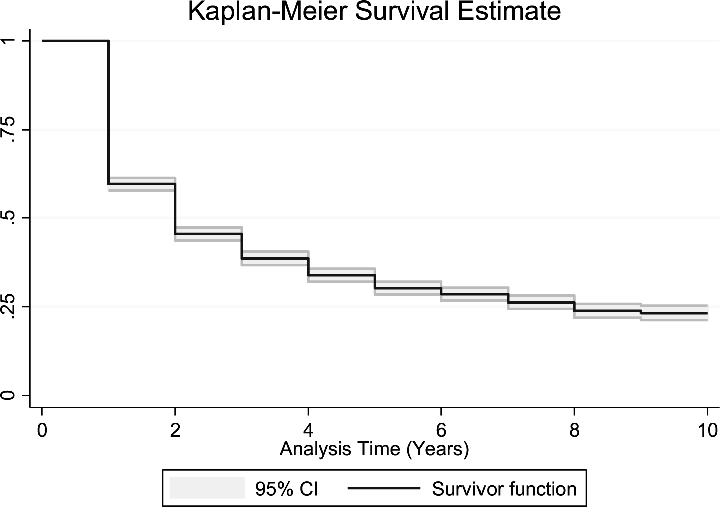
A review of the survivor functions in the life table (Table 2) easily demonstrates when the largest percentages of individuals were lost from the dataset. The survivor function after the first time period (0.5955) indicates that 40.45% were lost after just the first year. A survivor function of 0.4549 after the second year demonstrates that another 14.06% were lost in the second year, with only 45.49% of donors surviving after two years. However, the survivor function was reduced to only 0.3866 after the third time period and to only 0.3391 after the fourth, indicating that the function leveled off after the first two time periods. This phenomenon is depicted in Figure 1, a graphical representation of the survivor function over the 10-year period. Only 3.69% were lost after the fifth time period (equating to a survivor function of 0.3022) and only 1.71% dropped outafter the sixth (a survivor function of 0.2851). Overall, the life table indicates that after losing 54.51% of the individuals after the first two years, only 19.29% were lost over the subsequent five years, an average of only 3.86% each year.
Table 2
Life table describing durations of donor relationships
| Period | Time interval | Beginning total | Ended during period | Censored at end of period | Hazard function | Survivor function |
| 0 | [0, 1) | 2979 | — | — | — | 1.0000 |
| 1 | [1, 2) | 2979 | 1205 | 1774 | 0.4045 | 0.5955 |
| 2 | [2, 3) | 1656 | 391 | 1265 | 0.2361 | 0.4549 |
| 3 | [3, 4) | 1119 | 168 | 951 | 0.1501 | 0.3866 |
| 4 | [4, 5) | 805 | 99 | 706 | 0.1229 | 0.3391 |
| 5 | [5, 6) | 561 | 61 | 500 | 0.1087 | 0.3022 |
| 6 | [6, 7) | 424 | 24 | 400 | 0.0566 | 0.2851 |
| 7 | [7, 8) | 333 | 27 | 306 | 0.0811 | 0.2620 |
| 8 | [8, 9) | 239 | 22 | 217 | 0.0921 | 0.2379 |
| 9 | [9,10) | 163 | 4 | 159 | 0.0245 | 0.2320 |
| 10 | [10,11) | 87 | 0 | 87 | 0.0000 | 0.2320 |
| Overall | hazard rate | 0.2392 |
Note: Survivor function is calculated over full data and evaluated at indicated times; it is not calculated from aggregates shown at left.
Fig.1
Graph of survivor function for donor survival over time (with 95% CI).
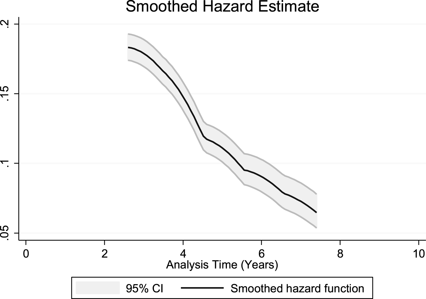
The hazard functions in Table 2 indicate when the probability of event occurrence was highest. Similar to the analysis of survivor functions, the highest hazard function was during the first time period, with a hazard function of 0.4045 indicating the probability of an individual exiting the dataset was 40.45%. The hazard functions then decreased, from 0.2351 after the second time period, to 0.1501 after the third, 0.1229 after the fourth, 0.1087 after the fifth, and 0.0566 after the sixth, as a smaller percentage of individuals exited the dataset in each subsequent time period. This is represented in Fig. 2, which depicts the hazard function sloping downward in a fairly linear fashion. There was a small increase in the hazard function after the seventh time period, as it rose to 0.0811 and to 0.0921 after the eighth. However, overall, the hazard functions depict that the probability of event occurrence was generally much lower the longer the individual remained in the dataset. These results conflict with those of Jensen & Turner (2017), who found that the probability of a sponsorship ending increased from the first to the second time period in two different datasets, with the hazard function the highest for both after the second year. The overall hazard rate is also depicted in the life table (0.2392). This corresponds to an overall probability of the donor’s relationship ending during any particular time period (23.92%). The hazard rate can also be utilized tocompute the organization’s overall renewal rate over the 10-year period (76.08%).
Fig.2
Graph of smoothed hazard function for donor survival over time (with 95% CI).
Finally, through analyzing the survivor functions in the life table depicted in Table 2, the median lifetime was computed. Given that the median lifetime is the point at which the survivor function is exactly 0.5 and the survivor function after the second time period is 0.4549, it is evident that the median lifetime occurred sometime between the first and second years. Using Miller’s (1981) formula, the median lifetime of athletic department donors was found to be 1.68. While in the case of this study the survivor function experienced the highest drop after the first year, the hazard function was also highest after the first year, and the survivor function equaled 0.5 during the first and second years, it is not always the case that these three metrics tell similar stories (Jensen & Turner, 2017; Singer & Willett, 2003).
5.2Semiparametric survival models
After the results of nonparametric survival models were analyzed, including the use of a life table to compute and examine survivor functions, hazard rates, and median lifetimes, we employed what Meyers et al. (2017) described as a semiparametric model. Using the aforementioned Cox proportional hazards model, covariates were inserted into the model to better understand how the various characteristics related to donors and the athletic department affect the probability of relationship dissolution. As noted, a systematic approach was utilized to ascertain whether groups of variables (economic, demographic, marketing, and athletic success) each predicted a statistically significant amount of the variance in the hazard for relationship dissolution. As indicated in Table 3, the group of control variables related to economic issues was inserted into the model first, to ensure that these variables were controlled for throughout the subsequent analysis. As expected, this grouping of variables did not predict a significant amount of the variance in the hazard for dissolution, χ2(3) = 1.57, p = 0.666.
Table 3
Hierarchical survival analysis modeling results
| Predictor Variables | Model 1 | Model 2 | Model 3 | Model 4 |
| Economic | ||||
| Lifetime Giving | –0.92 (0.00) | –1.01 (0.00) | 6.23 (0.00) | 6.36 (0.00) |
| Inflation | 0.43 (0.02) | 0.43 (0.02) | 1.28 (0.02) | 1.00 (0.02) |
| Economic Growth | 0.54 (0.02) | 0.63 (0.02) | –0.06 (0.02) | 0.82 (0.02) |
| Demographic | ||||
| Alumni | 1.53 (0.72) | 1.29 (0.57) | 1.23 (0.57) | |
| Live in State | –7.24** (0.04) | –7.23** (0.04) | –7.30** (0.04) | |
| Years since Graduation | –0.62 (0.00) | 0.99 (0.00) | 1.02 (0.00) | |
| Retired | –1.28 (0.07) | –2.77* (0.06) | –2.74* (0.06) | |
| Marketing | ||||
| Times Contacted | –5.78** (0.00) | –5.79** (0.04) | ||
| Athletic | ||||
| NCAA Tourney Wins | –2.82* (0.04) | |||
| Bowl Wins | 0.21 (0.07) | |||
| Log-likelihood | –6551.93 | –6633.79 | –6604.31 | –6600.83 |
| Wald χ² | 1.57 | 57.40** | 33.43** | 9.56* |
Results from Cox model, with the Breslow method for handling ties; Standard errors clustered by person. Standardized coefficients are listed, with standard errors in parentheses. *p < 0.01; **p < 0.001.
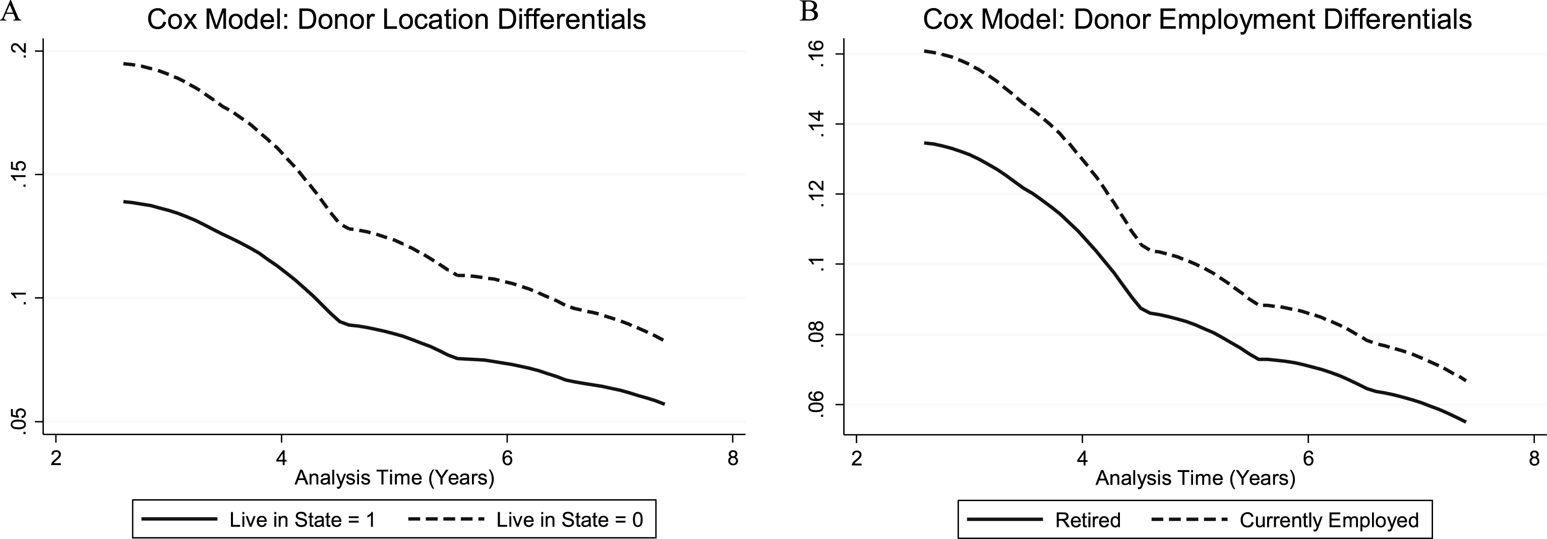
Next, in the second step, the grouping of demographic variables was inserted into the model. As displayed in Table 3, this group of variables did predict a significant amount of incremental variance, χ2(4) = 57.40, p < 0.001. In addition, the variable related to whether the individual lived in the same state as the university was highly significant, z = –7.30, p < 0.001. The coefficient’s hazard ratio (0.67) showed that the donor living in-state decreased the hazard of dissolution by 32.3%. The variable related to the donor’s employment status was also significant at the α= 0.01 level, z = –2.74, p = 0.006. The hazard ratio (0.82) demonstrated that being retired decreased the hazard for dissolution by 18.2%. Conversely, inserting a variable indicating that the person is actively employed serves to increase the odds that the relationship will end, z = 2.77, p = 0.006, with a hazard ratio of 1.22 indicating it increased the hazard for dissolution by 21.9%. The effects of both of these variables are depicted graphically in Fig. 3, which illustrates the differential in the hazard function over time based on whether the individual lives in the same state or not (Graph A) and whether he or she is actively employed (Graph B). The marketing-related variable was then inserted into the model, reflecting the effect of the number of times donors were contacted by the athletic department. The results included in Table 3 reveal a significant effect, z = –5.79, p < 0.001. The hazard ratio of 0.98 shows that each time the individual was contacted by the athletic department the probability of the relationship ending decreased by 1.6%.
Fig.3
Graphs of smoothed hazard functions based on differentials for donor location (Graph A) and employment status (Graph B).
Finally, the grouping of variables reflecting the on-field performance of the athletic department in each season was inserted. This group of variables also predicted a significant amount of the variance, χ2(2) = 9.56, p = 0.008. The variable reflecting success in men’s basketball was significant at the α= 0.01 level, z = –2.82, p = 0.005. The hazard ratio (0.87) indicated that each win for the men’s basketball team in the NCAA championship tournament decreased the probability of ending the relationship by 12.84%. The variable reflecting football success, which indicated a win in a postseason bowl game, was nonsignificant.
6Discussion
This project applied survival analysis modeling to quantitatively analyze and predict the potential dissolution of the intercollegiate athletic department-donor relationship, utilizing 10 years of data from a mid-sized NCAA FBS athletic program. For athletic development officers, understanding the timing and circumstances surrounding when it is most imperative to allocate resources toward relationship-building efforts with donors is critically important. Prior research attempting to inform donor relationship management revealed a donor’s motivations, but failed to account for the athletic development department’s potential role in donor retention, and had yet to predict the timing and conditions when it would be most critical for an athletic development officer to stress donor relationship cultivation. Study results inform a data-driven approach to donor relationship management, provide meaningful implications for athletic donor retention strategy, and the analysis offers a template for future data-driven decision investigation regarding potential customer retention problems.
Results demonstrate that the athletic department-donor relationship is most susceptible to dissolution in the first two years (just over half defected in this time period). This conclusion reflects evidence in sport management literature suggesting sport season ticket holders in their first or second year are far more likely to defect in comparison with longer standing season ticket holders (Irwin et al., 2008 p. 133). In the instance that intercollegiate athletic development departments spend a disproportionate amount of time and resources on nurturing relationships with its longer-term donors, the results of this study suggest that managers might instead be wise to focus their energy toward the first two critical years of the donor relationship. Athletic development directors could direct their energy in the form of specialized stewardship programs for new donors knowing that the donor is increasingly likely to persist regardless of economic changes as each subsequent year passes.
Although athletic department-donor contact decreases the hazard for relationship dissolution only slightly (just over one percent), this small but significant result is a start to understanding the impact an athletic development department can have on donor retention. Knowing that touchpoints can make a difference in retention efforts, athletic development directors and teams may find it time well spent to form a coordinated set of outreach to donors especially around the vulnerable first and second relationship years. Although not a direct byproduct of this investigation, the result inspires the investigation into how touchpoints serve as a catalyst for other important donor behaviors, such as upgrade, or the reinstatement of a lapsed donor. An opportunity exists to further operationalize the types and quality of interactions (face-to-face versus receiving a direct mail piece) as well as donor participation in other stewardship activities (e.g. special coach meet and greets).
As athletic development offices employ short and long-term donor retention goals and strategy, survival analysis modeling results reveal qualities potentially affecting a donor’s lifetime value to the organization. Results suggest that the act of retiring actually reduces the hazard for relationship dissolution, which for some may be a counterintuitive result. However, it makes sense that donors who are currently employed are busier and have less time to devote, which may result in gaps in their relationships with the university. Retirees may naturally have lifestyles conducive to supporting athletic donor relationship longevity, for example, a fixed and expected income as well as more time to attend athletic-related and other university events. A similar case can be made for in-state residents; a closer location creates a convenience for university integration. These situational factors that ease participation with the university showed increased importance to donor longevity, in comparison with variables of perceived importance such as alumni status or years from graduation. In fact, results revealed that alumni status was surprisingly understated in the model. Donors who were not alumni, such as faculty, staff, and members of the community, were just as likely to have long-term relationships with the university athletic program as alumni. In addition, winning also mattered more than alumni status to donor retention, specifically regarding the progression and advancement of the men’s basketball team into post-season play. The notion that football bowl game wins were non- significant may be a reflection of the saturation of bowl offerings or may be a reflection of the culture at the school, that men’s basketball is more important to donors and potentially, the athletic culture at large.
Applying the results of the study to short-range donor recruitment and retention efforts will refocus the energy of athletic development staff to the recruitment and protection of early relationships with those donors living in-state, as well as those who have retired. These relationships are more likely to persist over the long term. Specialized stewardship events for early donors focused for segments with disposable incomes, time to devote, and located at a convenient distance to the university may be a worthy investment. Knowing that men’s basketball success is important to donor retention, the athletic development department can preplan efforts and resources to leverage and capitalize on a successful men’s basketball post- season. Long-range planning for this particular organization should address tactics to improve how the athletic development department reaches and retains alumni and other natural stakeholders in order to further develop and retain the donor base. Decisions affecting short- and long-term planning will also be a function of the access the development office has to these key groups.
6.1Limitations
It should be noted that while the data analyzed in this study are from an institution that participates at the highest level of NCAA designation (the Football Bowl Subdivision), it is not a member of one of the five major athletic conferences (i.e., the Power Five). Thus, these results may not be generalizable to those NCAA institutions playing in the Atlantic Coast Conference, Big Ten, Big 12, Pac-12 Conference, or Southeastern Conference. The results may also not be generalizable to institutions with different historical records of athletic success; fan base expectations and reactions to athletic success achievement may vary. It is recommended that the modeling approaches utilized in this study be applied to data from a Power Five institution or to institutions with different athletic success histories, to investigate whether the results generalize to institutions competing at other levels. In addition, while these data were longitudinal in nature, only 10 years of data were available for analysis. In the future, we recommend that the survival of the donor relationship be analyzed over a period of longer than 10 years. Finally, in this study we were necessarily limited to an examination of the explanatory variables that were tracked by the athletic department over the 10-year period. There may be supplementary covariates that could prove to be significant predictors, but the effects of which were unable to be analyzed in this study, including other demographic variables such as education orhousehold income.
6.2Future research
Multi-venue research incorporating additional covariates will inform a more efficient and effective customer retention process. Given the advances of customer relationship management platforms, it is recommended that athletic departments collect and future analyses include further variables that might unearth additional insights for those seeking to maximize donor retention. Within the context of athletic donors, this could include behavioral variables such as collecting ticket and merchandise purchasing patterns, giving level, patterns of university integration, additional demographic variables such as gender, as well as operationalizing the quality of athletic department-donor interactions. While the geographic location of the donor was noted in the model based on whether or not the donor resided in the same state as the university, a continuous variable indicating the donor distance from campus would be a preferred approach for measuring the impact of this distance on relationship dissolution. For the intercollegiate athletic environment, specifically, this analysis could also be applied to the length of time that an institution spends in an athletic conference, and the factors that may affect that duration.
This study offers impactful conclusions for FBS athletic departments and serves as a template for future and wide-ranging applications of survival analysis modeling to sport customer relationship management, for customers at all levels of sport including single and season ticket sales buyers, health club attendees, corporate sponsors and beyond. Where retaining customers is an organizational goal, applying survival analysis can be instrumental to informing successful customer relationship strategies.
Acknowledgments
We would like to acknowledge our sport organization partners for opening their data warehouses for this research project and others. We would also like to thank the organizers and attendees of the 2017 Great Lakes Analytics in Sports Conference for their helpful suggestions and the confidential journal article reviewers of the Journal of Sports Analytics for their effort and valuable feedback throughout the review process.
References
1 | Aulakh P.S. , Kotabe M. and Sahay A. , (1996) , Trust and performance in cross-border marketing partnerships: A behavioral approach, Journal of International Business Studies, 27: (5), 1005–1032. |
2 | Baade R.A. and Sundberg J.O. , (1996) , Fourth down and gold to go? Assessing the link between athletics and alumni giving, Social Science Quarterly, 77: (4), 789–803. |
3 | Barro R.J. , (1991) , Economic growth in a cross section of countries, The Quarterly Journal of Economics, 106: (2), 407–443. |
4 | Bolger N. , Downey G. , Walker E. and Steininger P. , (1989) , The onset of suicidal ideation in childhood and adolescence, Journal of Youth and Adolescence, 18: (2), 175–190. |
5 | Boskin M.J. , Dulberger E.R. , Gordon R.J. , Griliches Z. and Jorgenson D.W. , (1998) , Consumer prices, the consumer price index, and the cost of living, Journal of Economic Perspectives 12: (1), 3–26. |
6 | Box-Steffensmeier J.M. and Jones B.S. , (1997) , Time is of the essence: Event history models in political science, American Journal of Political Science 41: (4), 1414–1461. |
7 | Box-Steffensmeier J.M. and Jones B.S. , (2004) , Event History Modeling: A Guide for Social Scientists. Cambridge: University Press. |
8 | Cobbs J. , Tyler B.D. , Jensen J.A. and Chan K. , (2017) , Prioritizing sponsorship resources in Formula One Racing: A longitudinal analysis, Journal of Sport Management, 31: (1), 96–110. |
9 | Cooney N.L. , Kadden R.M. , Litt M.D. and Getter H. , (1991) , Matching alcoholics to coping skills or interactional therapies: Two-year follow-up results, Journal of Consulting and Clinical Psychology, 59: (4), 598–601. |
10 | Cox D.R. , (1972) , Regression models and life tables, Journal of the Royal Statistical Society 34: (2), 187–220. |
11 | Drayer J. , Shapiro S.L. and Lee S. , (2012) , Dynamic ticket pricing in sport: An agenda for research and practice, Sport Marketing Quarterly, 21: , 184–194. |
12 | Fry M.J. and Ohlmann J.W. , (2012) , Introduction to the special issue on analytics in sports, Part 1: General sports applications, Interfaces, 42: , 105–108. |
13 | Fulks D.L. , (2016) , Revenues and Expenses, 2004–2015: NCAA Division I intercollegiate athletics programs report, http://www.ncaa.org/sites/default/files/2015%20Division%20I%20RE%20report.pdf. |
14 | Furby L. , Weinrott M.R. and Blackshaw L. , (1989) , Sex offender recidivism: A review, Psychological Bulletin, 105: (1), 3. |
15 | Gladden J.M. , Mahony D.F. and Apostolopoulou A. , (2005) , Toward a better understanding of college athletic donors: What are the primary motives? Sport Marketing Quarterly, 14: , 18–30. |
16 | Grimes P.W. and Chressanthis G.A. , (1994) , Alumni contributions to academics, American Journal of Economics and Sociology, 53: (1), 27–40. |
17 | Hoang H. and Rascher D. , (1999) , The NBA, exit discrimination, and career earnings, Industrial Relations: A Journal of Economy and Society, 38: (1), 69–91. |
18 | Irwin R.L. , Sutton W.A. and McCarthy L.M. , (2008) , Sport Promotion and Sales Management, (2nd ed.). Human Kinetics: Windsor, ON. |
19 | Jensen J.A. and Turner B.A. , (2017) , Advances in sport sponsorship revenue forecasting: An event history analysis approach, Sport Marketing Quarterly, 26: (1), 6–19. |
20 | Jensen J.A. and Cornwell T.B. , (2017) , Why do marketing relationships end? Findings from an integrated model of sport sponsorship decision-making, Journal of Sport Management, 31: (4), 401–418. |
21 | Kaplan E.L. and Meier P. , (1958) , Nonparametric estimation from incomplete observations, Journal of the American Statistical Association, 53: (282), 457–481. |
22 | Ko Y.J. , Rhee Y.C. , Walker M. and Lee J. , (2014) , What motivates donors to athletic programs: A new model of donor behavior, Nonprofit and Voluntary Sector Quarterly, 43: (3), 523–546. |
23 | Mahony D.F. , Gladden J.M. and Funk D.C. , (2003) , Examining athletic donors at NCAA Division I institutions, International Sports Journal, 7: (1), 9–27. |
24 | Martinez J.M. , Stinson J.L. , Kang M. and Jubenville C.B. , (2010) , Intercollegiate athletics and institutional fundraising: A meta-analysis, Sport Marketing Quarterly, 19: , 36–47. |
25 | Mazodier M. and Rezaee A. , (2013) , Are sponsorship announcements good news for the shareholders? Evidence from international stock exchanges, Journal of the Academy of Marketing Science 41: (5), 586–600. |
26 | Meyers L.S. , Gamst G. and Guarino A.J. , (2016) , Applied Multivariate Research: Design and Interpretation. Thousand Oaks: Sage Publications. |
27 | Miller R.G. , (1981) , Survival Analysis. New York: Wiley. |
28 | Myers R.H. , (1990) , Classical and Modern Regression with Applications. Boston: PWS-KENT. NCAA Research, 2016, Eleven-year Trends in Division I Athletics Finances, http://www.ncaa.org/sites/default/files/DivisionI_ElevenYearFinances-20150917.pdf. |
29 | Nevo D. and Ya’acov R. , (2012) , Around the goal: Examining the effect of the first goal on the second goal in soccer using survival analysis methods, Journal of Quantitative Analysis in Sports, 9: (2), 165–177. |
30 | Paul R. and Weinbach A. , (2013) , Determinants of dynamic pricing premiums in Major League Baseball, Sport Marketing Quarterly, 22: , 152–165. |
31 | Pierce D.A. , Popp N. and McEvoy C. , (2017) , Selling in the Sport Industry. Dubuque, Iowa: Kendall Hunt. |
32 | Popp N. , Barrett H. and Weight E. , (2016) , Examining the relationship between age of fan identification and donor behavior at an NCAA Division I athletics department, Journal of Issues in Intercollegiate Athletics, 9: , 107–123. |
33 | Rhoads T.A. and Gerking S. , (2000) , Educational contributions, academic quality, and athletic success, Contemporary Economic Policy, 18: (2), 248–258. |
34 | Shank M.D. , (2009) , Sports marketing: A strategic perspective (4th ed.). Pearson Prentice Hall: Upper Saddle River, NJ. |
35 | Shapiro S.L. and Ridinger L.L. , (2011) , An analysis of donor involvement, gender, and giving in college athletics, Sport Marketing Quarterly, 20: , 22–32. |
36 | Singer J.D. and Willett J.B. , (2003) , Applied Longitudinal Data Analysis: Modeling Change and Event Occurrence. Oxford: University Press. |
37 | Spector P.E. and Brannick M.T. , (2011) , Methodological urban legends: The misuse of statistical control variables, Organizational Research Methods, 14: (2), 287–305. |
38 | Staw B.M. and Hoang H. , (1995) , Sunk costs in the NBA: Why draft order affects playing time and survival in professional basketball, Administrative Science Quarterly, 40: , 474–494. |
39 | Stinson J.L. and Howard D.R. , (2008) , Winning does matter: Patterns in private giving to athletic and academic programs at NCAA Division I-AA and I-AAA institutions, Sport Management Review, 11: (1), 1–20. |
40 | Tsiotsou R. , (2007) , An empirically based typology of intercollegiate athletic donors: High and low motivation scenarios, Journal of Targeting, Measurement, and Analysis for Marketing 15: (2), 79–92. |
41 | Tucker I.B. , (2004) , A reexamination of the effect of big-time football and basketball success on graduation rates and alumni giving rates, Economics of Education Review 23: (6), 655–661. |
42 | Turner S.E. , Meserve L.A. and Bowen W.G. , (2001) , Winning and giving: Football results and alumni giving at selective private colleges and universities, Social Science Quarterly 82: (4), 812–826. |
43 | The World Bank Group, (2017) , The World Bank Data Catalog [Data file], data.worldbank.org |


