
Factors associated with match outcomes in elite European football – insights from machine learning models
Abstract
AIM
To examine the factors affecting European Football match outcomes using machine learning models.
METHODS
Fixtures of 269 teams competing in the top seven European leagues were extracted (2001/02 to 2021/22, total >61,000 fixtures). We used eXtreme Gradient Boosting (XGBoost) to assess the relationship between result (win, draw, loss) and the explanatory variables.
RESULTS
The top contributors to match outcomes were travel distance, between-team differences in Elo (with a contribution magnitude to the model half of that of travel distance and match location), and recent domestic performance (with a contribution magnitude of a fourth to a third of that of travel distance and match location), irrespective of the dataset and context analyzed. Contextual factors such as rest days between matches, the number of matches since the managers have been in charge, and match-to-match player rotations were also shown to influence match outcomes; however, their contribution magnitude was consistently 4–8 times smaller than that of the three main contributors mentioned above.
CONCLUSIONS
Machine learning has proven to provide insightful results for coaches and supporting staff who may use their results to set expectations and adjust their practices in relation to the different contexts examined here.
1Introduction
Football is a total social phenomenon (Defrance, 2009), i.e., one of the only phenomena, if not the only one, that involves all the societal institutions –social, cultural, economical and political. There are more than 250 million participants worldwide. Since the early 1980s, soccer has greatly evolved in many different aspects (e.g., venue design, laws of the match, competition formats) (Brocherie, 2020). As a result of an increasing match, sponsorship, and broadcasting revenue, the industry witnessed exponential growth (e.g., fan engagement and athlete performance technology support). A dramatic increase in player salaries, market values, and net transfer expenses has been reflected in this growth (Quansah, 2021). Soccer transfers, for instance, are an example of this –fees reached a record of USD 7.4 B in 2019, almost a tripling of what they were in 2012 (FIFA, 2019). As recently as January 2023, there were more than 14.4% more transfers and 49.9% more transfer fees agreed than in January 2022 (FIFA, 2023).
Overall, winning in football has never mattered more than today. Understanding the factors that may be associated with winning matches, may shed light into the complex question of success in elite football. While things will always depend on the context, several factors have, in isolation, already received some attention in the literature. While a given team formation (Buchheit, 2023a) and running performance per se (Modric, 2023) may not be directly associated with success, it’s likely the coaches’ ability to adapt their match plan to each opponent that makes more the difference –but this is unlikely an easy task to isolate and examine this at the macro level. Among the ‘simple’ factors the most examined, the effects of the number of rest days between matches (Buchheit, 2022; Verheijen, 2012) and match location (González-Rodenas, 2019, Lago-Peñas, 2016; Pollard, 1986) are probably the most straightforward, with teams tending to lose more often when travelling away with few days of rest between matches –even though the best teams with large squad (and ability to rotate players while maintaining their playing quality (O’Hanlon 2020), may actually deal better with these difficult scenarios (Buchheit, 2022; Settembre, 2023). Other factors including team ranking (González-Rodenas, 2019), manager changes (Radzimiński, 2022), players availability (Hägglund, 2013; Eliakim, 2020) and player management strategies such as substitutions (Buchheit, 2023c) and rotations (Settembre, 2023; Bekris, 2020; Schmidt, 2017) play also a role.
To our knowledge, while modelling match outcomes is not new (Berrar, 2019; Maher, 1982; Wheatcrof, 2021), how all these factors interact altogether has not been examined comprehensively; and whether those factors influence performance in different contexts is also unknown e.g. different leagues, competitions or club standards. The aim of this study was therefore, to examine the interaction of multiple factors that can affect match outcomes using data from the seven best European leagues and machine learning models, i.e., Extreme Gradient Boosting (XGBoost) for Classification (Settembre, 2023). More precisely, we first looked at all available data together, regrouping the last 21 seasons (i.e., from the 2000/01 to the 2021/22 seasons). Considering some teams use domestic cups and UEFA Europa Conference League matches to rotate their players, we only included the following main competitions: domestic leagues, UEFA Champions League (CL) and Europa League (EL) including their qualifying phases. We then looked at those factors at different levels: decades (2000s and 2010–2020s), groups of competitions (all domestic leagues and major European cups i.e. CL and EL), single competitions (each domestic league, CL and EL separately); and finally team levels (top 10% teams when playing against each other and non CL/EL teams).
2Methods
2.1Data extraction
We extracted the fixtures data of teams competing in the top seven European leagues, i.e., the English Premier League (EPL), the French Ligue 1, the German Bundesliga, the Dutch Eredivisie, Italian Serie A, the Portuguese Liga and Spanish Liga. This includes 21 seasons from 2001/02 to 2021/22. The fixtures from all in-season competitions were considered, i.e., leagues and domestic, European and international cups. This data was sourced from Transfermarkt. Across the 21 seasons, this represents 43 competitions, 269 teams and more than 61,000 fixtures.
2.2Model-based analysis
Based on the above-mentioned fixtures data extract, the following metrics were used to identify the key factors that could impact teams performance:
• Rest days: number of days between matches, irrespective of the competition. For instance, playing on Wednesday after a previous match on Sunday gives two rest days (Monday and Tuesday). When data was erroneously entered in the online database (e.g., 2 games played the same day), data was changed to NaN and treated as a missing value (0.01% of the dataset).
• Travel distance: distance as the crow flies between the 2 ground locations.
• Number of matches since the manager started his position (only when the manager stayed more than 5 matches)
• Domestic performance to date: percentage of league points won since the season started.
• Recent performance: percentage of points won during the last 5 matches (all competitions) (Radzimiński, 2022)
• Number of rotations compared to the previous match (all competitions considered) (Bekris 2020; Schmidt 2017)
• Lineup rolling stability: it assesses starting line-up variation during the last 5 matches. Considering that teams have different squad sizes which impacts the metric and its comparison from one team to another, we defined a max squad size of 45 players (max size in the dataset). We then created 45 –N “fake” players per team, N being the squad size (McHugh, 2023)
• Team’s Elo rating: its definition is based on the standard Elo rating formula and our own assumptions (Settembre, 2023).
• Team status:when a team plays the CL and/or EL during a given season, they get the status of CL and/or EL teams during the whole season, no matter when they go out of the competition.
• Team league
• Location: home or away
• Information about the previous match:
∘ Travel distance
∘ Location
∘ Competition: split into 4 groups
■ Domestic leagues
■ Major international cups: CL/EL (qualifying phase included), UEFA Super Cup and FIFA Club World Cup.
■ Minor international cups: UEFA Intertoto Cup (until 2009) and Europa Conference League (qualifying phase included)
■ Domestic cups
Difference with opposition team for numerical metrics:
∘ Rest days
∘ Number of matches since manager started
∘ Domestic performance to date
∘ Recent performance
∘ Number of rotations
∘ Distance traveled for the previous match
∘ Rolling stability
∘ ELO rating
Sixteen groups of data were used for the final analysis (all regrouping data from the 2000/01 to the 2021/22 seasons). The 16 different models run were the following:
• Main competitions all together: domestic leagues, UEFA Champions League (CL) and Europa League (EL) including their qualifying phases.
• Decades (i.e., 2000–2010 and 2011–2021)
• Groups of competitions (all domestic leagues and major European cups i.e. CL and EL),
• Single competitions (each domestic league, CL and EL separately)
• Team levels (top 10% teams when playing against each other and non CL/EL teams). The top 10% teams are those teams having an ELO rating greater than 1624, which is the 90th percentile of ELO rating over the whole period.
For the total 20 year period considered there were approximately 53,000 fixtures, with about 24,000 fixtures in the first decade (2001/02 to 2009/10) and 29,000 in the second (2010/11 to 2021/22). Domestic league fixtures accounted for 47,000 fixtures, while there were ∼6,100 fixtures from the Champions League and Europa League competitions. Using the ELO rating we defined the top 10% teams as those having an ELO rating greater than 1624, the 90th percentile of ELO rating over the whole period. When limiting to top teams playing against each other we had about 880 fixtures. The level of missing data was not about 5% for most metrics and always <12%. Missing data was mostly observed in international cup fixtures, and almost only for the teams not playing in the top 7 leagues (weaker teams). We did not remove fixtures with missing data and let the model handle those cases as the level was the same for the training and test sets.
In order to study the relationship between result (win, draw, loss) and the explanatory variables, we used eXtreme Gradient Boosting (XGBoost) for Classification. We focused on the Win class to analyse the factors related to performance.
Even if multicollinearity has no impact on performance of XGBoost models by nature, it does affect feature importance. Thereby, we studied the Pearson correlation between all pairs of features. The largest positive correlation value was between Difference Elo and Difference Domestic Performance to Date (0.76), while the largest negative one was between Home and Travel Distance (−0.77). Considering that there was no very strong (positive or negative) correlation between any pairs of features, we decided to keep all of them in the model.
When looking at the overall context, the level of missing data per metric goes from 0 to 10%. Information about competitions and Elo is almost fully complete while the other metrics related to a team has 1 to 5% of missing data. For metrics related to the difference with the opposition team, this doubles i.e. up to 10%. This lack of data mainly comes from teams that are not part of the top 7 European leagues, supposedly weaker. This phenomenon then impacts less league-focused models i.e. less than 5% of missing data for each metric, while being more present for models based on European matches (30 to 60% of missing data). Considering that the data is missing not at random and this pattern is the same in the training and test sets, its impact on the model accuracy is not significant (Rusdah & Murfi, 2020). We then decided to run all models without imputation on them.
As teams played in empty stadiums from COVID restart in May 2020 to the end of the 2020/21 season—impacting the home-field advantage—we decided to exclude this period from the analysis. For the overall model (main competitions), we then split the data set into training and test sets based on the following seasons:
• Training set (80% of the data): from 2001/02 to 2016/17
• Test set (remaining 20%): from 2017/18 to 2021/22 excluding the COVID period
We built the training and test sets of the other contexts following this 80% /20% rule.
The XGBoost model structure is defined by hyper-parameters. In order to get the optimal ones, we used a randomised grid-search based on the training set. A grid-search runs through all the different parameters fed into the parameter grid and produces their best combination based on a scoring metric. A randomised grid-search does not try all combinations out but rather a fixed number of iterations, i.e., 20 here. It then returns a relatively accurate performing model in a significantly shorter runtime (Bergstra, 2012). The parameter grid considered is the following one:
• Number of iterations: 20
• Model evaluation: accuracy
• Cross-validation (CV) splitting strategy: 5-fold CV
• Step size shrinkage: 0.1*, 0.15, 0.2
• Subsample ratio of columns when constructing each tree: 0.3, 0.5*, 0.7
• Maximum depth of a tree: 3*, 7, 15
• Number of trees: 20, 100*, 500
• L1 regularisation term on weights: 0.1, 10, 50*
The values with an asterisk are the optimal ones for the overall model.
To explain how our model works, i.e. the decisions it is making, we used SHapley Additive exPlanations (SHAP) values (Lundberg & Lee, 2017). SHAP does this by using fair allocation results from cooperative game theory to allocate credit for a model’s output among its input features. Its calculation involves averaging the marginal contributions of each player (or feature) across all potential permutations of players (features). This involves assessing every possible combination of features and determining the impact each feature has on the model’s prediction when included in these combinations. By averaging these contributions across all possible feature arrangements, it achieves a balanced and interpretable evaluation of each feature’s importance in the model’s prediction. One of the fundamental properties of SHAP values is that all the input features will always sum up to the difference between baseline (expected) model output and the current model output for the prediction being explained. In the case of binary classification the sum of the feature SHAP values equals the prediction log-odds, while for multiclass classifications the softmax function is used. As such the individual SHAP values are difficult to interpret by themselves. As our task is defined from a team perspective, we implemented a 3-class classification: win, draw or loss. We then decided to study the following concepts related to the “win” class i.e. the factors that contribute to teams’ success:
• Feature Importance: based on the absolute SHAP values per feature, it analyses the global importance of each feature. For a given prediction each feature will have a positive or negative SHAP value indicating whether it positively or negatively contributes towards the predicted value. The absolute SHAP value is a measure of how important the feature is irrespective of its direction, and so taking its average across all predictions provides a global measure of how important a feature is to the model.
• Feature Relationship: it indicates the relationship between the value of a feature and the impact on the prediction.
• Feature Dependence: as an alternative to partial dependence plots and accumulated local effects, it focuses on a given feature and shows for each data instance the relationship between the feature value (x-axis) and the corresponding SHAP value (y-axis).
Based on this Feature Dependence concept, we created a modified version of the SHAP dependence plot (Lundberg, 2018) (i.e., all Figures showing univariate results). One dot is the SHAP value (y-axis) related to an actual observation of a given metric (x-axis) –e.g. travel distance –within a given context i.e. match here. For instance, for many matches, travel distance is equal to 500 kms multiple times. This does not mean that all of these points get the same SHAP value as they come from different matches. For each game, travel distance = 500 kms can have a different impact on the expected result depending on the other metrics’ value. When the feature (x-axis) is non-binary, local trends between two non-binary entities are shown using locally-linear estimated scatterplot smoothing (LOESS) and its 95% prediction intervals (PI). We defined four zones to summarise the impact of the feature on match-to-match rotations:
∘ Increasing: both the LOESS curve and PI are above 0
∘ Likely increasing: the LOESS curve is above 0 but 0 is included in PI
∘ Likely decreasing: the LOESS curve is below 0 but 0 is included in PI
∘ Decreasing: both the LOESS curve and PI are below 0
For binary features, a box plot is used. It is based on the SHAP values related to each instance (0 and 1), and the same parameters as the ones defined in the above-mentioned Descriptive Analysis subsection. The four zones are created as follows:
∘ Increasing: both the median and interval between whiskers (WI) are above 0
∘ Likely increasing: the median is above 0 but 0 is included in the WI
∘ Likely decreasing: the median is below 0 but 0 is included in the WI
∘ Decreasing: both the median curve and WI are below 0
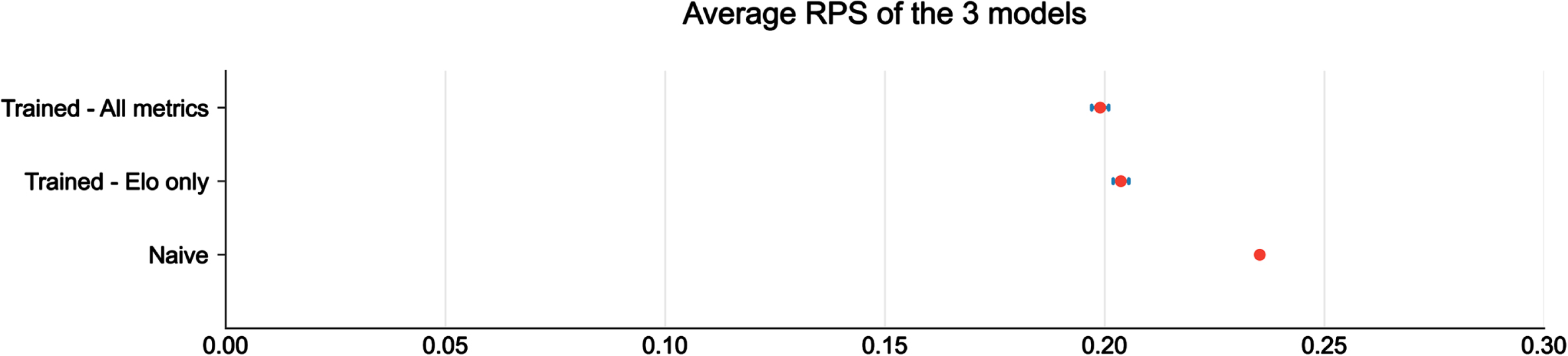
Finally, we evaluated the probabilistic prediction of an individual match using the ranked probability score (RPS). In order to assess the model performance on the entire test set, we defined the average over all RPS related to each match in this set. The smaller the average RPS, the better the predictions (Berrar, Lopes & Dubitzky, 2019). We compared our model trained on all listed features with:
• Naive model: all predictions are the relative frequencies of wins, draws and losses in the training set.
• Elo model: all predictions are calculated from a model only trained on Elo and Difference Elo variables. We chose Elo as it is often the most important feature for our models. This then enabled us to study the significance of the impact of the other variables.
Knowing that the model performance can vary depending on the test set, we generated 95% confidence intervals (CI) for the average RPS by bootstrapping the test set. As seen on Fig. 1, the full model related to the overall context (main competitions) performs better than both the naive and Elo models, with an average evaluation of 0.1990, 95% CI being [0.1971, 0.2009]. Even if our training and test sets are different from the ones of the 2017 Soccer Prediction Challenge, this model performance is better than the one from the challenge winners Team OH whose average RPS was 0.2063.
Fig. 1
Average Ranked Probability Score of the model trained on all metrics, the one trained only on Elo variables and the naive one.
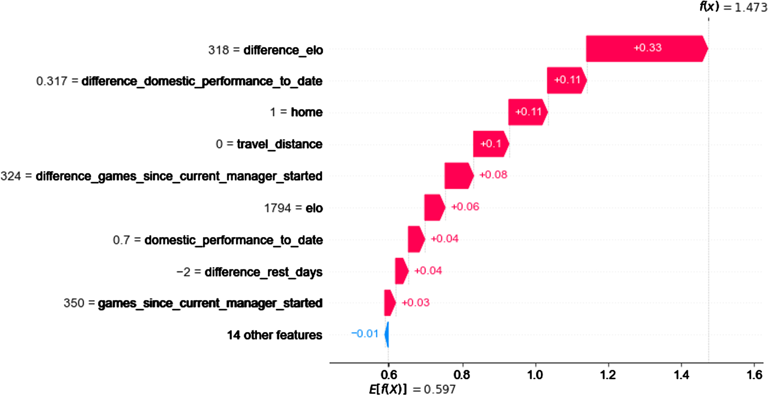
We use SHAP to interpret the model predictions. Its additive nature allows each prediction to be split out into the contributions from each feature in the model over and above the SHAP expected value, and ranked in order of importance / magnitude.
The SHAP expected value is essentially the frequency of a team winning the game across the training set. Considering our multi-class classification, the softmax function should be applied to this number in order to transform it into an understandable one. The softmax function turns a vector of K (K = 3 here) real values into a vector of K real values that sum to 1. The expected value of winning is 0.597 here, which translates to a frequency of winning the game for each team (without taking the home-field advantage into account) of 36.6%. Figure 2 shows how SHAP is used to interpret the model prediction of Liverpool winning their game at home against Brentford on January 16, 2022. The combined SHAP contributions plus the expected value gives the resulting prediction, 1.473 in this case which gives a 69.3% chance of winning the game. The main contributor here was the Elo difference between Liverpool and their opponents i.e. 318 before the match. It added a contribution of 0.33 in addition to the expected value. The contribution of the other features is shown in Fig. 5. Liverpool actually won that game 3-0.
Fig. 2
SHAP contribution of each feature on Liverpool performance for their game at home against Brentford on January 16, 2022.
3Results
Given the extensive amount of results, we first provided the detailed feature relationship plot for the main data set (i.e., main competitions, Figs. 3 and 4).
Fig. 3
Feature importance plot for main competitions (main model, all data pooled together). This shows the relative contribution of the top variables the model uses to estimate match outcomes.
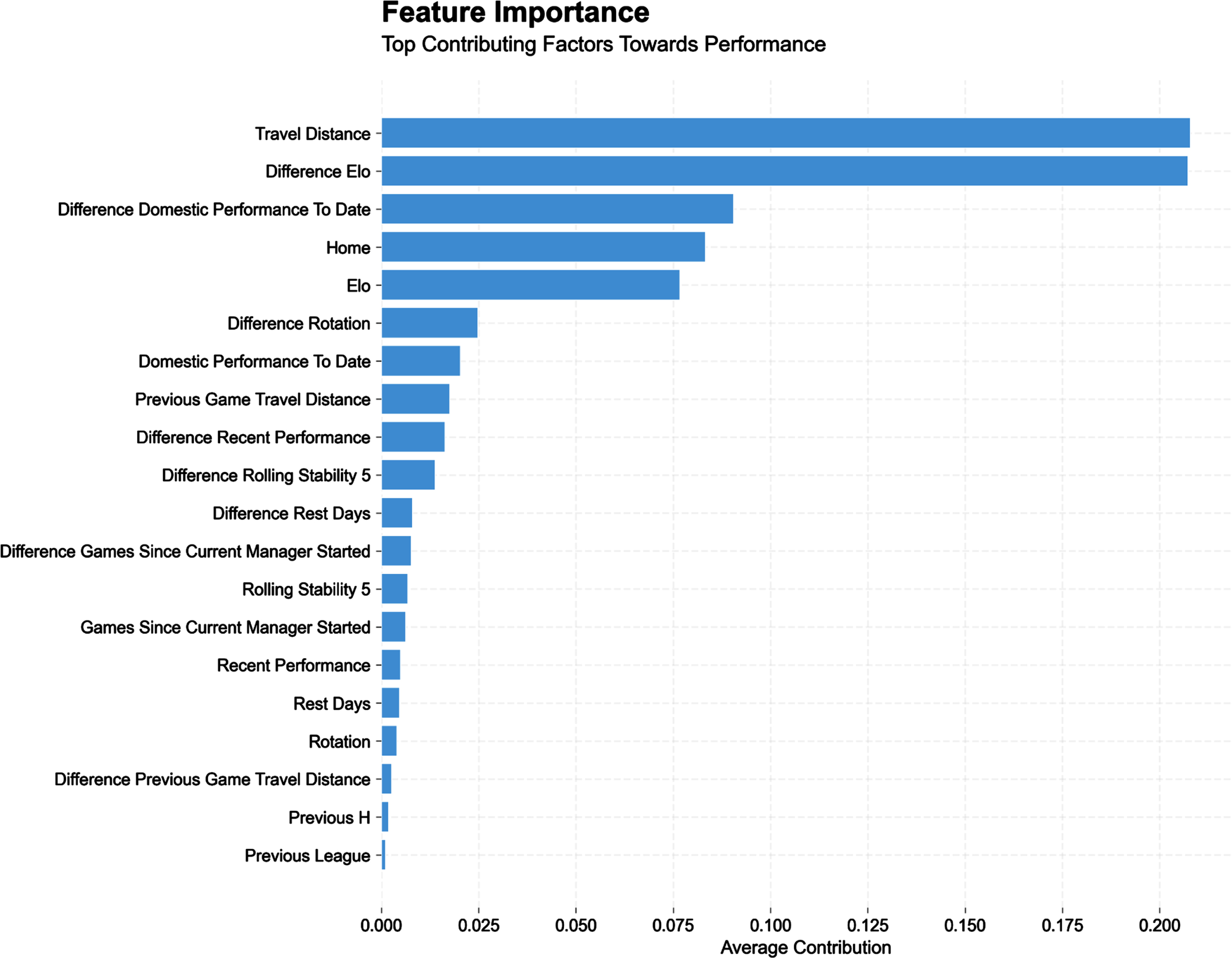
Fig. 4
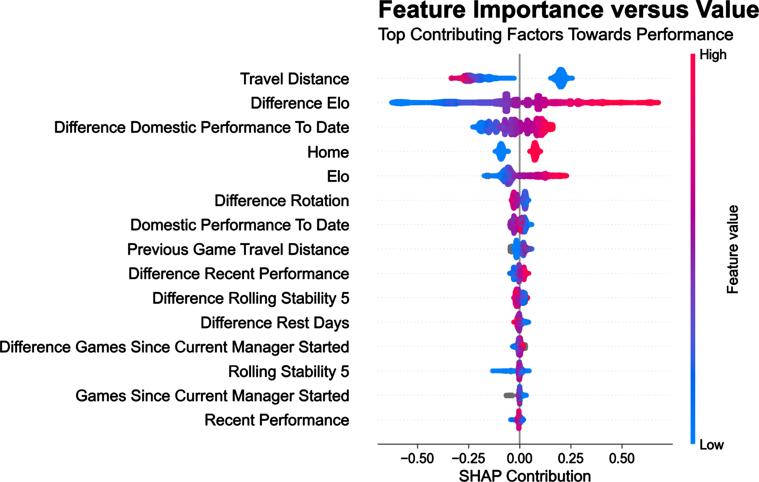
Feature Relationship plot for main competitions (all data pooled from all leagues and over the 21 seasons). This shows in detail the SHAP contribution from the model’s most important metrics, shown in Fig. 3, to each match outcomes estimate. Each data point (team-match) is shown, and for each metric data point, low values are shaded in blue, and high values in red. If a data point is to the right of the centre line, i.e., a positive SHAP contribution, then it is associated with increased performance and vice versa.
The complete set of results (i.e., Feature relationship plots, Figs. 5 and 6 and univariate SHAP dependency plots, Figs. 7–12) were then only provided when analyzing performance of the 10% best teams playing against each other.
Fig. 5
Feature Importance plot for the 10% best teams playing against each other (i.e., teams with an Elo superior to 1624, Elo’s 90th percentile). This shows the average SHAP contribution from the most important metrics to the model’s match outcomes estimates.
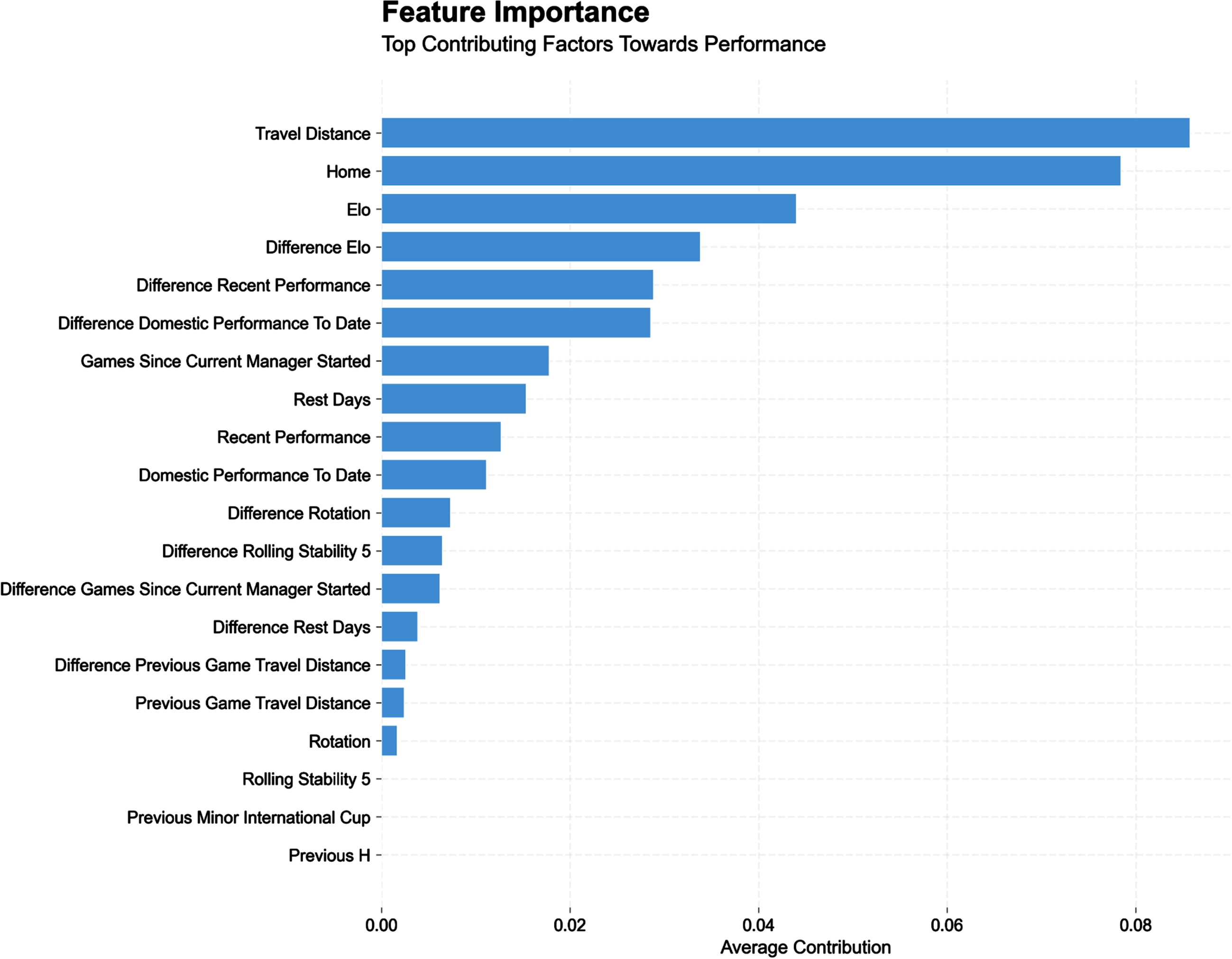
Fig. 6
Feature Relationship plot for the 10% best teams (i.e., teams with an Elo superior to 1624, Elo’s 90th percentile) playing against each other. This shows in detail the SHAP contribution from the model’s most important metrics, shown in Fig. 5, to each match outcomes estimate. Each data point (team-match) is shown, and for each metric data point, low values are shaded in blue, and high values in red. If a data point is to the right of the centre line, i.e., a positive SHAP contribution, then it is associated with increased performance and vice versa.
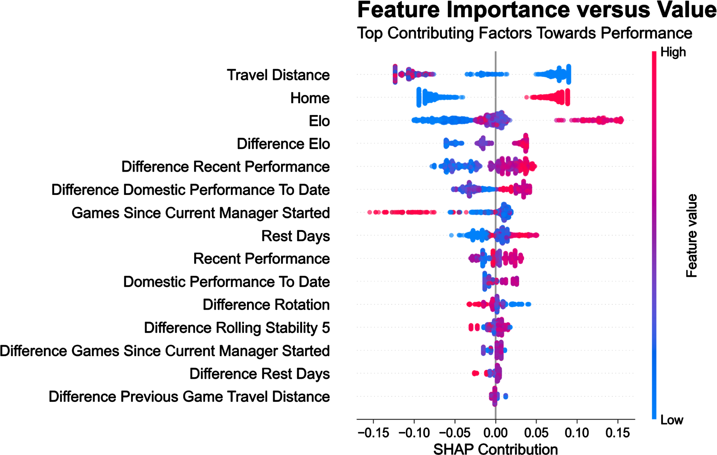
Fig. 7
SHAP dependency plots for travel distance (left) and match location (right). Travel distance plot has been truncated at 500 km in order to have a better view of its low values. The observations from 500 to 2500 km follow the same trend as that seen from 300 to 500 km i.e., red zone with a flat line. Performance (+/−) is quantified as the magnitude of the SHAP contribution.
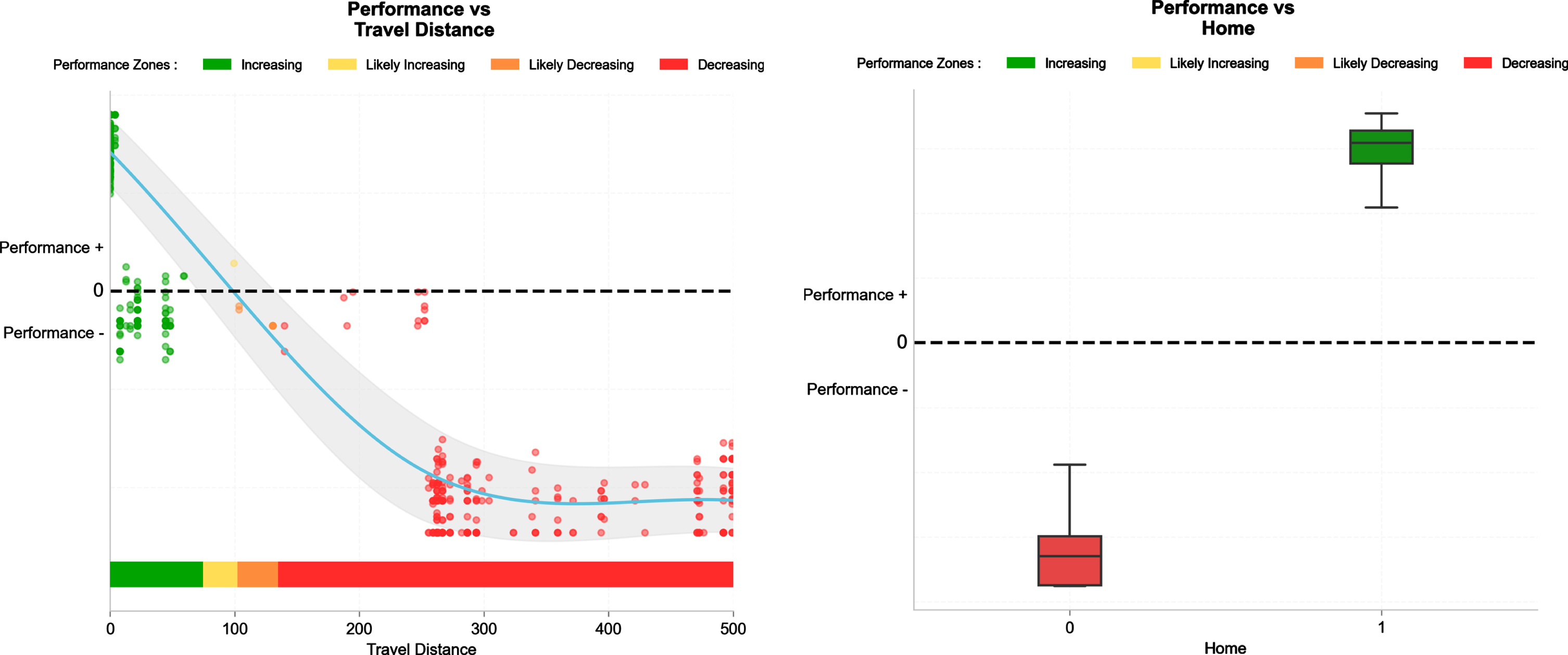
Fig. 8
SHAP dependency plots for the difference in Elo vs. the opponent (left) and the team’s Elo (right). Performance (+/−) is quantified as the magnitude of the SHAP contribution.
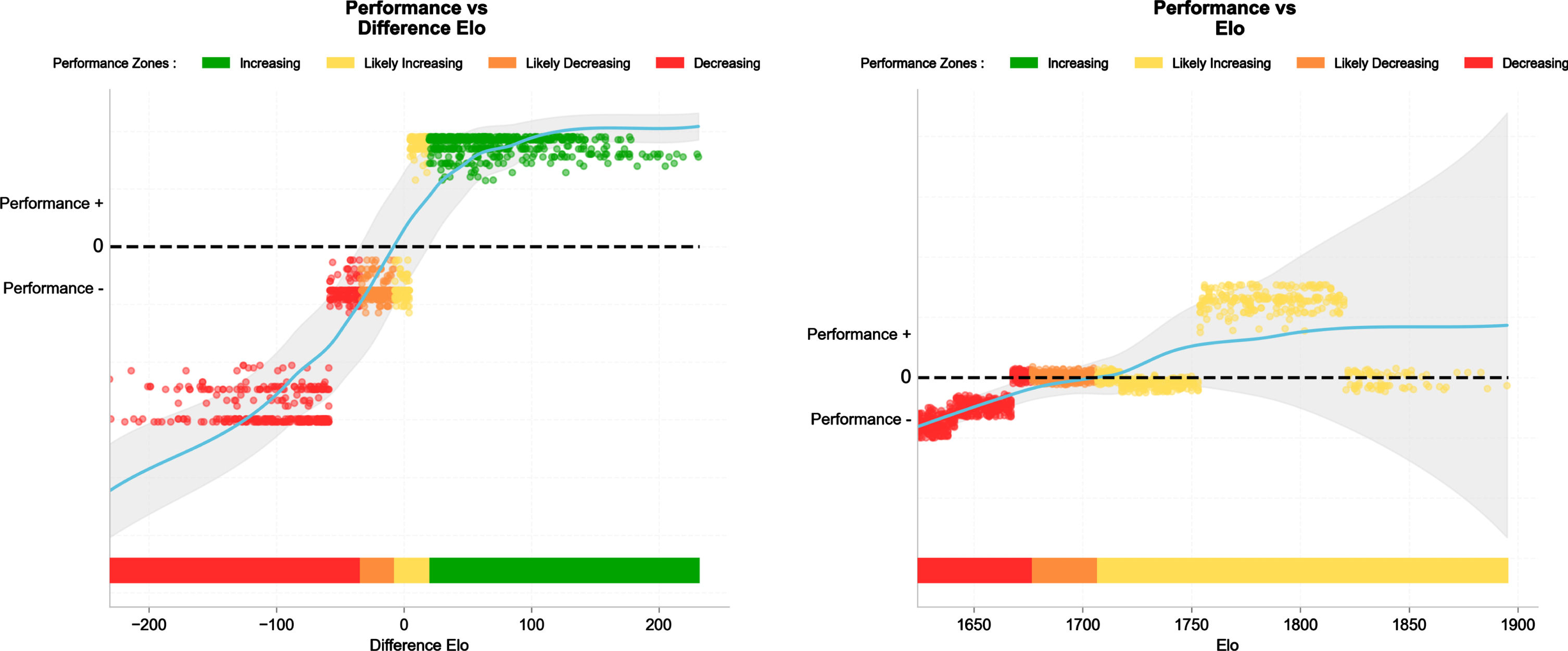
Fig. 9
SHAP dependency plots for domestic performance to date (percentage of points won since the start of the season within the domestic league, left panels) and recent performance (percentage of points won during the last five matches all competitions included, right panels).
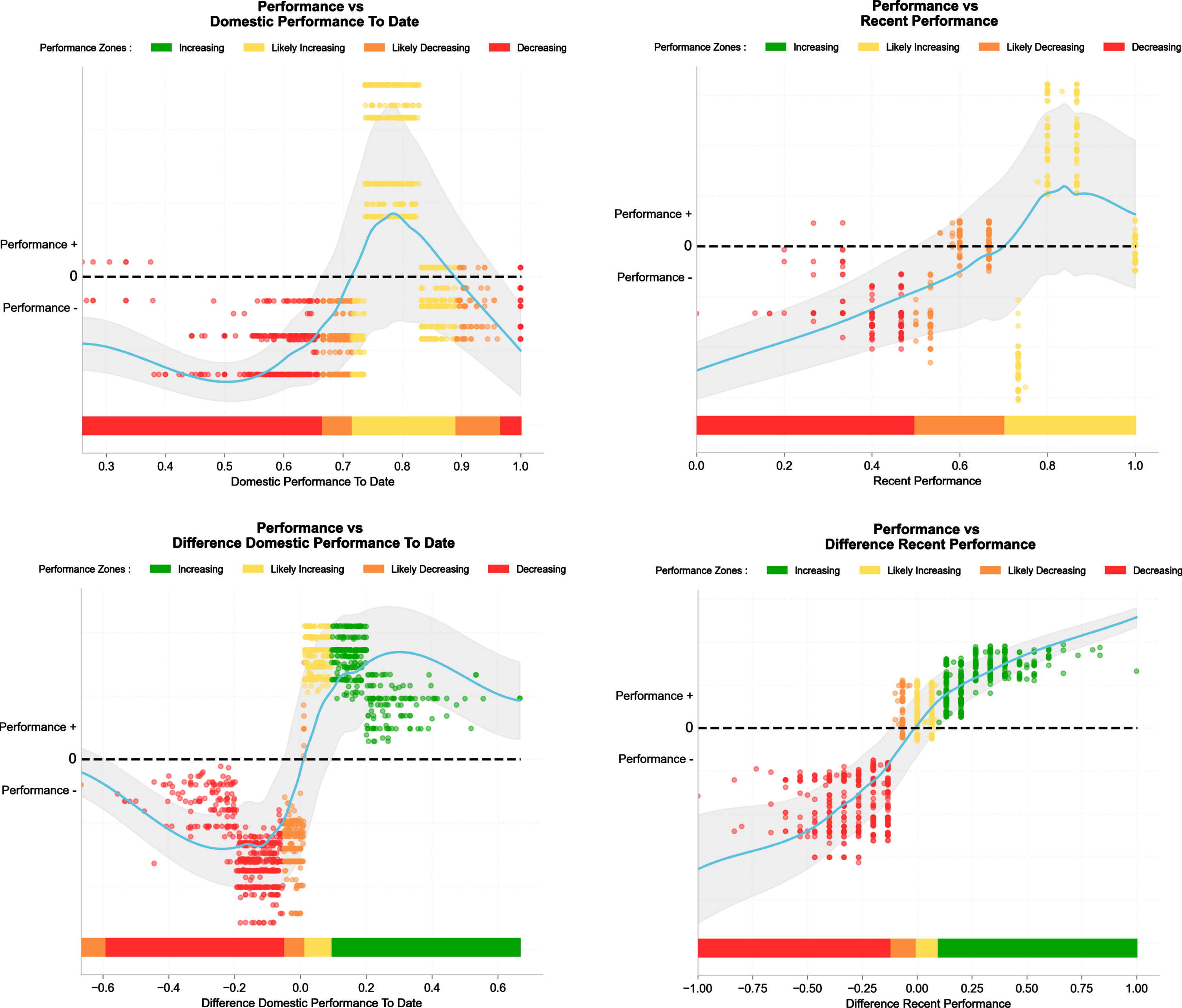
Fig. 10
SHAP dependency plots for the number of matches since the manager started.
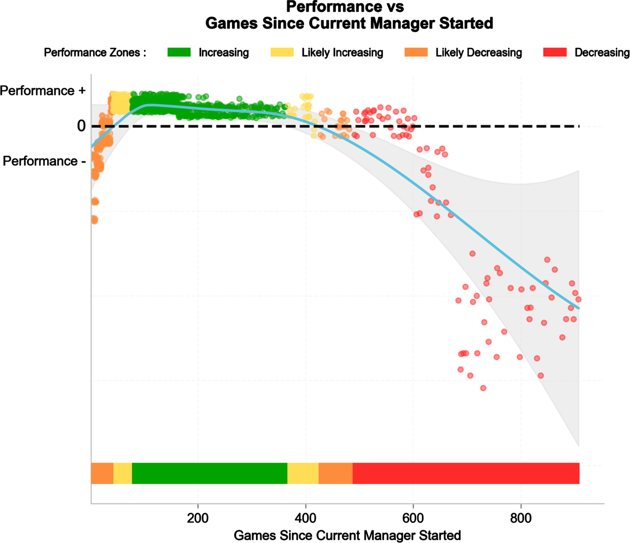
Fig. 11
SHAP dependency plots for the absolute number of rest days (i.e., the number of days separating two consecutive matches, left panel) and the difference in rest days between the two teams (right panel). Performance (+/−) is quantified as the magnitude of the SHAP contribution.
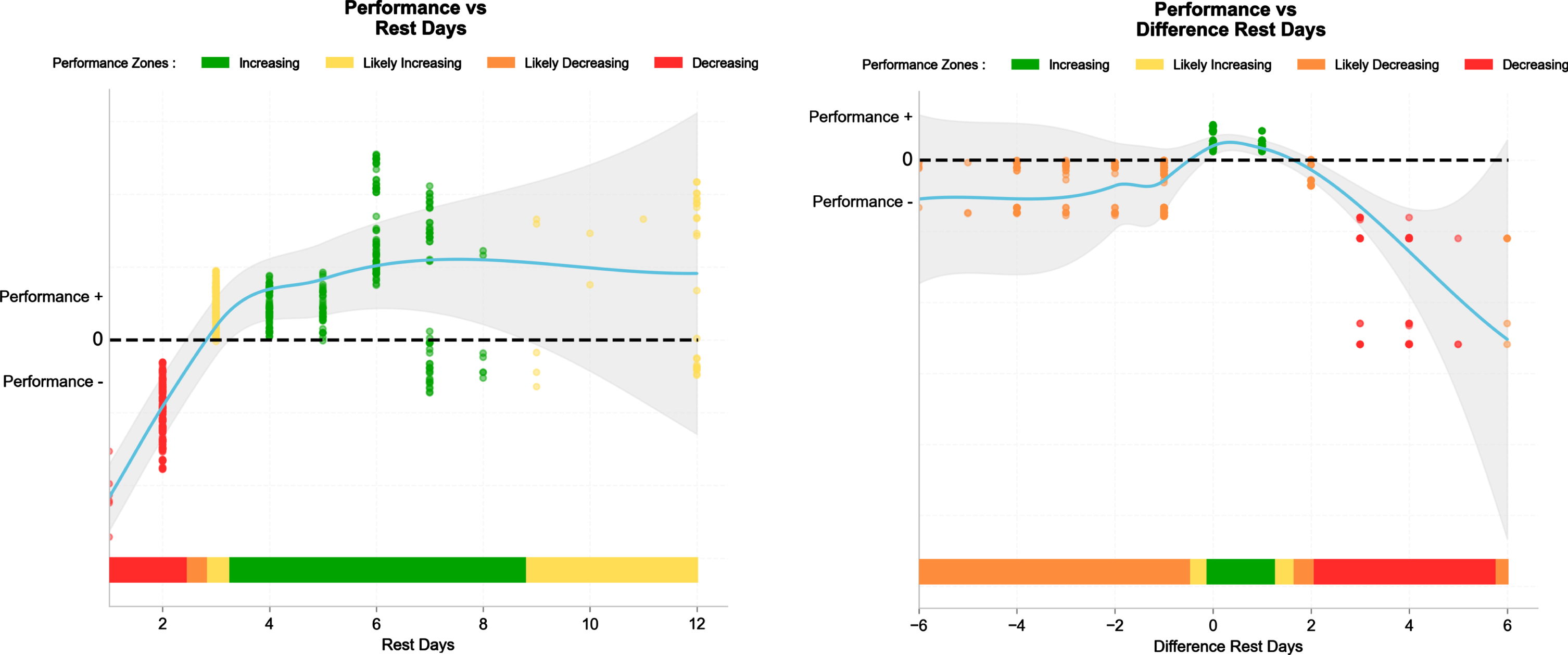
Fig. 12
SHAP dependency plots for differences in rotations between the teams (match-to-match rotation from the previous, left) and rolling stability (right). Performance (+/−) is quantified as the magnitude of the SHAP contribution.
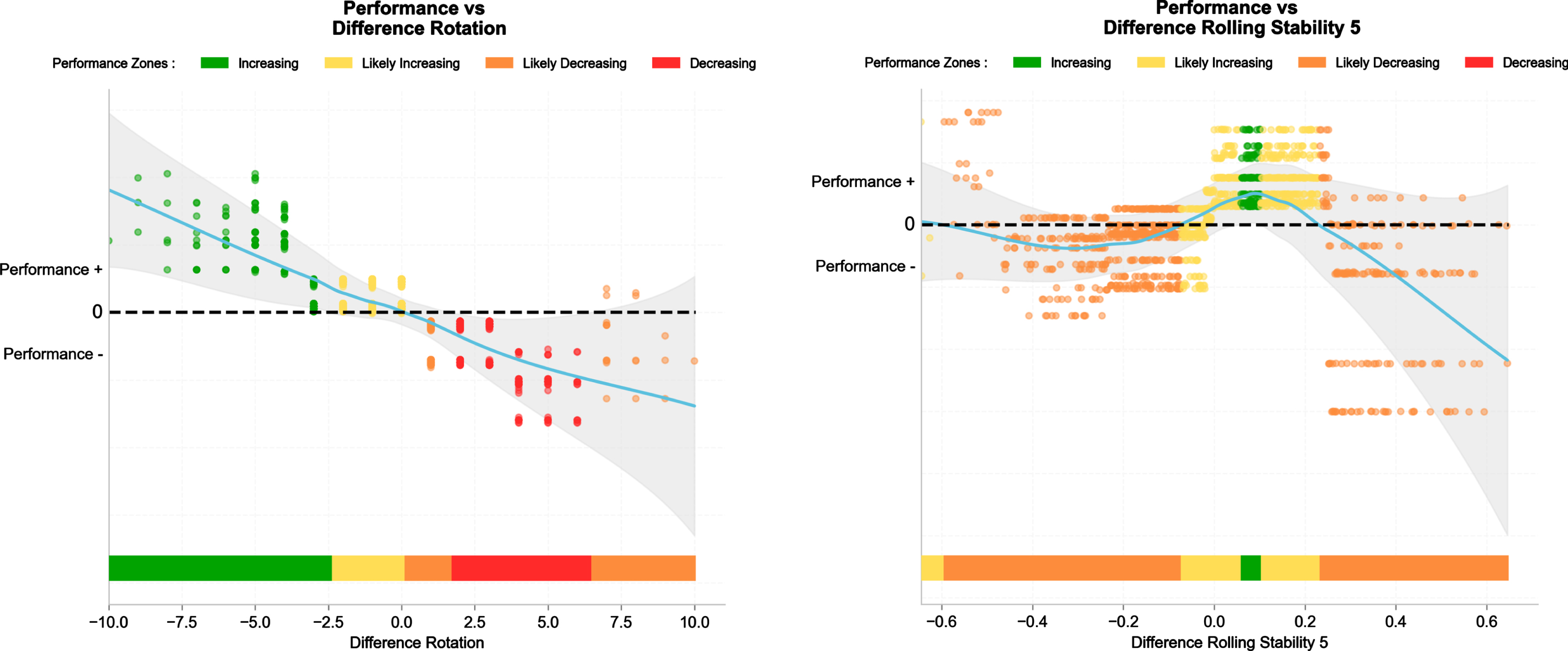
Table 1 summarises the five top variables contributing to all models. The key factors that affected match outcomes were ranked in relation to their respective contribution to the models –with difference in Elo (often more than Elo itself), travel distance (often more than location per se) and recent (domestic) performance being consistently the top contributors, irrespective of the dataset and context analyzed. Players management including match-to-match rotations and line-up stability, and contextual factors such as rest days between matches and the number of matches since the managers have been in charge were also shown to influence match outcomes; however, their magnitude of contribution was also consistently small in comparison to the three above.
Table 1
Ranking of the Top 5 contributing variables across 16 different models run. For example, Travel distance was ranked as the first contributing factor for 10 of the 16 models and second one for 6 of them
| 1 | 2 | 3 | 4 | 5 | |
| Travel Distance | 10 | 6 | |||
| Diff Elo | 6 | 9 | 1 | ||
| Elo | 6 | 4 | 5 | ||
| Location | 1 | 4 | 4 | 5 | |
| Diff Domestic Performance To Date | 3 | 7 | 2 | ||
| Matches Since Manager Started | 2 | 1 |
The SHAP dependency plots in Fig. 7 show that while performance is decreased away (right panel), travel distances > 100 km are likely to affect performance.
The contribution of Elo to team performance was straightforward, with match outcomes being increased as soon as the absolute difference in Elo vs. the opponent was positive (Fig. 8, left panel). There was also a tendency for top teams (Elo > 1700, right panel Fig. 8) to perform better than others.
Figure 9 shows various associations between actual match outcomes and differences in both domestic performances to date (bottom left) and differences in recent performance (bottom right). In practice, top teams that have been performing better (>0% of possible points) than their opponents both in their domestic league since the start of the season (bottom left) and over the last five matches (bottom right) showed improved performance. Performance (+/−) is quantified as the magnitude of the SHAP contribution.
The contribution of the number of matches the manager has been in charge is shown in Fig. 10. In this latter model, teams had poorer performance when playing with a recently-appointed (<30 matches) or long-established (>420 matches) manager. Performance (+/−) is quantified as the magnitude of the SHAP contribution.
The data confirm that performance is clearly impaired with only two days of rest even in the top 10% teams playing against each other. They also show that it’s only with > 3 days of recovery that top teams seem to regain their expected competitive advantage (Fig. 11, left panel).
Teams performed better when they presented fewer rotations (i.e.,<0) from the previous match than the opponent (Fig. 12 left panel). However, the association with line-up stability over the past 5 matches was unclear (Fig. 12, right panel).
4Discussion
Our current results add to the existing literature (Berrar, 2019; Maher, 1982; Wheatcrof, 2021), providing an updated view on how football match outcomes can be modelled, here using XGBoost for Multi-class Classification. The full model related to the overall context (main competitions) performed better than both the naive and Elo models, with an average evaluation of 0.1990, 95% CI being [0.1971, 0.2009]. Even if our training and test sets were different from the ones of the 2017 Soccer Prediction Challenge, this model performance was better than the one from the challenge winners Team OH whose average RPS was 0.2063. Bookmakers’ RPS have been shown in some studies to be around 0.16, however this is not surprising given bookmakers can update their odds right up until a match kick-off using information that is not included e.g. team news, last-minute injuries, weather conditions etc (Hubáček et al., 2018).
Looking across all model predictions, the SHAP contributions for all metrics in the model can be used to provide insight into the key factors affecting match outcomes in general. In Figs. 4 and 6, they are ranked in relation to their respective overall contribution to the model, either positive or negative when considering the entire period, and the main competitions.
The contribution of the different factors is discussed by their order of magnitude across the different models (Table 1), following a special reference to the most interesting model, i.e., what happens for the 10% best teams when playing against each other. The top contributors to match outcomes were travel distance (often more than location per se), between-team differences in Elo (often more than the Elo itself) (with a contribution magnitude to the model half of that of travel distance and match location), and recent (domestic) performance (with a contribution magnitude of a fourth to a third of that of travel distance and match location), irrespective of the dataset and context analyzed (Table 1). Contextual factors such as rest days between matches and the number of matches since the managers have been in charge, and players’ management strategies including match-to-match rotations and line-up stability, were also shown to influence match outcomes; however, their magnitude of contribution was also consistently 4 to 8 times smaller than that of the three above (Figs. 3 and 5).
4.1.Match location and travel distance
The average contribution to the 10% best teams model was slightly higher for travel distance (0.085) than location (0.078) (Fig. 5); their contribution magnitude was however twice that of the second sets of metrics (i.e; Elo, see below). The SHAP dependency plot in Fig. 7 shows that while match outcomes were clearly decreased away (right panel), it’s essentially the away matches that require to travel over distances >100 km that was really likely to affect performance (left panel) equivalent to a drive of 1 h–1 h30 maximum in bus. The substantial and important effect of match location is in agreement with the commonly reported home-field advantage (Pollard, 1986; Lago-Peñas, 2016). While there remains some inconsistency in the literature, we recently reported a clearly lower likelihood to win for away vs. home (expected 30% vs. 45% wins, Buchheit, 2022 & 2023b) within the same present data set. Among all the possible factors explaining the home-advantage, travel fatigue and crowd support were shown to contribute less to home advantage than do the less easily quantifiable benefits of familiarity with conditions when playing at home (Lago-Peñas, 2016).
4.2Elo
The contribution of Elo to team performance was straightforward (with an overall contribution to the 10% top teams model of 0.045, Fig. 5), with top teams (Elo > 1624, right panel Fig. 8) performing better than others. Performance was also increased as soon as when the absolute difference in Elo vs. the opponent was positive (Fig. 8, left panel) (contribution of 0.035, Fig. 5). These findings are logical are confirm the relevance of this index as a measure of overall team quality. The direct application of these findings is that coaches may expect ‘easier’ wins when playing teams of clearly lower Elo, and may use this as an opportunity to rotate/rest players when needed (i.e., congested periods).
4.3Difference in recent performance and domestic performance to date
The overall contribution of team performance (recent and to date) to the 10% best teams model ranged from 0.015 to 0.030 (Fig. 5). We observed various associations between actual match outcomes and differences in both domestic performance to date (bottom left, Fig. 5) and differences in recent performance (bottom right, Fig. 5). In practice, top teams that have been performing better (>0% of possible points) than their opponents both in their domestic league since the start of the season (bottom left) and over the last five matches (bottom right) showed improved performance. While overall team performance (since 1980 for our algorithm, Settembre, 2023) is used to produce the Elo rating (discussed above), the inclusion of these short- (five last matches) and long-term (performance to date since the start of the season) metrics was aimed at capturing the actual ‘form’ of each team which carries some sort of performance momentum. Anecdotally, this recent performance over the most 5 recent matches (Radzimiński, 2022) is also used in many sport websites for the general population of readers (i.e., google sport results). It is worth noting that we used a generic definition of ‘recent performance’, which can be interpreted as good or bad for a particular team depending on their context at the time. For example, a team in the relegation zone would be described as being in ‘good form’ if they picked up 10 points from 5 games, but for a title-chasing team the same outcome would probably be considered ‘bad form’. We chose this approach with practicality in mind since the quality of performance is team-dependent and may also change with time (and seasons). Defining ‘recent performance’ at the team level is a topic for future investigation.
4.4Managers
The contribution of managers lifespan to the 10% best team model was 0.017 (Fig. 5), i.e., half of that of Elo and a fourth of travel distance and match location. Interestingly, the number of matches since the manager was in charge was ranked as a substantial contributor to performance in many models. It was in the Top 3 in the teams in European cups (Table 1), and in 7th position in the top 10% teams model (Figs. 5 and 6). In this latter model, teams had a poorer performance when playing with a recently-appointed (<30 matches, which are likely played over a little bit less than one season approximately) or long-established (>420 matches, which can represent >7 years) manager. The 30 matches mark is consistent with the idea that coaches need around a season to build their team tactics and game model, and confirms the results of a recent study when the influence of coach replacement was examined (Radzimiński, 2022). They actually reported that the highest number of collected points per game are obtained by coaches who lead their teams for several seasons. In contrast, these results also showed that while changing the coach during the soccer season may result in short-term improvement in team results and physical match performance, after a period of approximately 5 games, this effect disappears (Radzimiński, 2022).
While it’s also intuitive that coaches’ influence may decline over prolonged time (e.g., lack of new insights, decreased player motivation and engagement in relation to management style), the 8-year mark on the right side of the graph (Fig. 10) may be at first perceived at odd with current practices, where the majority of coaches last only a few seasons (e.g., the average life-span of managers ranges between 772 days, which is a little over two years and one month in the EPL, 628 days in the Bundesliga, 617 days in La Liga, and just 385 and 384 days in Ligue 1 and Serie A, respectively) (Price, 2022). A closer look at the graph (fewer data points) suggest that this trend is essentially reflective of the rare exceptions of managers who reached that milestone; the lower precision of the model at this point (as shown by the large CI around the main regression line) may be considered when interpreting this trend.
4.5Rest days
While only ranked as the 10th and 8th contributing factor when looking at all competitions together (Fig. 3) or only at the top 10 teams (with contribution to the model of 0.05 to 0.015, Fig. 5), respectively, the contribution of rest days (Fig. 11) was straightforward and consistent with previous studies (Buchheit, 2022; Verheijen, 2012). The data confirm that performance is clearly impaired with only two days of rest (e.g., playing on Wednesday and then again on Saturday, Fig. 12, left panel) even in top teams that may have more options to rotate players (Buchheit, 2022). Further than the potential physical and mental fatigue that may not be completely recovered within 48 h (Nedelec, 2012), we also observed that when playing the next match within less than three rest days, match-to-match rotations were increased (Settembre, 2023). In this complex context, coaches may rotate more players than usual to avoid increasing their risk of injuries (Page, 2023), which as discussed above, decreases between-player communication, and in turn, match outcomes.
It’s only with ≥4 days of recovery that top teams seem to regain their expected competitive advantage (in relation to their status and Elo, see above) (Buchheit, 2022). Along the same lines, it’s when these top 10% of teams had ≥1 rest day less than their opponents that they tend to underperform (Fig. 11, right panel).
4.6Line-up stability and match-to-match rotations
The contribution of line-up stability and match-to-match rotations to the 10% best teams model was around 0.010 for each metric (Fig. 5), i.e., a third of that of Elo and a eighth of travel distance and match location. Teams performed better when they presented fewer rotations (i.e., <0) from the previous match than their opponent (Fig. 12 left panel). The detrimental effect of player’s rotations is straightforward, considering that line-up stability favours better between-player communication (Verheijen, 2022) and in turn, match outcomes. In a previous study examining the effect of rotation on the performance of Champions’ League teams playing three matches a week (2014–15 to 2017–18 competitive season), more points in the domestic league were lost when a large number of players participated in the initial list for the three games. Similarly, increasing rotations in the initial list between the 1st and the 3rd game and between the 2nd and the 3rd game had a negative effect on the domestic league performance (Bekris, 2020). A specific analysis of 98 different teams in the “Top 5” European domestic leagues over the 2016–17 season showed more contrasted results however (i.e., lack of clear correlations between rotation numbers and performance); this lead the author to suggest that the effect of rotations per se is more complex than and that and likely related to a myriad of other factors (e.g., opposition, travels –which gives more credit to the present multi-factorial analysis), and should be relied upon on a case-by-case basis (Schmidt, 2017). For instance, in another study (Settembre, 2023), we showed that rotations were slightly increased when playing away, which may be related to the change in tactics that often occur away, with teams shifting toward more defensive team formations (Buchheit, 2023a). In accordance with the typical home-field advantage (e.g., crowd support, familiar environment, no travel, etc.) (Pollard, 1986; Lago-Peñas, 2016), this increased number of rotations when playing away may also partially explain the lower likelihood to win (expected 30% vs. 45% wins, for away vs. home, Buchheit, 2022). The current understanding about rotations, is that there is in fact a tradeoff between line-up stability and load management (i.e., to preserve players’ health, especially when playing congested); deciding how many players to rotate from one match to the next, and who to rotate remains a key question for every manager (O’Hanlon, 2020).
4.7Limitations
The main limitation of the current analysis remains the data set obtained from an online database. This data set constrained the factors included in the modelling part, since there may be other factors that were not available from Transfermarkt, whose influence could therefore not be examined. We have not compared our results with other machine learning techniques that are applicable to the problem (ordinal logistic regression, k-nnand etc.). While performance improvements are possible with those approaches we are satisfied with the approach given its performance relative to other studies. Finally, our study involved an analysis of various contexts to assess the potential variation of factors across different scenarios. These contexts were deliberately designed for comparative purposes, spanning decades (comparing the first with the second), groups of competitions (domestic leagues versus European competitions), single competitions (contrasting one league with another, as well as the UEFA Champions League with the UEFA Europa League), and specific team levels versus the entirety of available data. Importantly, our methodology ensured no cherry-picking of data. In this paper, we present a comprehensive summary of all 16 contexts, a broader perspective drawn from the complete dataset, and a detailed exploration of the specific context surrounding the top 10% of teams. This approach aims to provide a thorough understanding of how factors may evolve or differ in diverse contexts.”
5Conclusions and key findings
This is to our knowledge the first time that match outcomes has been modelled, here using XGBoost for Multi-class Classification. Looking across all model predictions, the SHAP contributions for all metrics in the model were used to provide insight into the key factors affecting match outcomes in general.
The top contributors to match outcomes were travel distance (often more than location per se), between-team differences in Elo (often more than the Elo itself, and with a contribution magnitude to the model half of that of travel distance and match location), and recent (domestic) performance (with a contribution magnitude of a fourth to a third of that of travel distance and match location), irrespective of the dataset and context analyzed.
Contextual factors such as rest days between matches and the number of matches since the managers have been in charge, and players’ management strategies including match-to-match rotations and line-up stability, were also shown to influence match outcomes; however, their magnitude of contribution was also consistently 4 to 8 times smaller than that of the three main contributors mentioned above.
In the top 10% of best teams when playing against each other, team performance is increased at the highest end when the strongest teams (Elo > 1624) teams play:
1. Home or within less than 100 km of distance
2. Against an opponent with an Elo of at least 10 points lower
3. Against an opponent with a poorer overall recent performance (>0% of possible points won over the last five matches)
4. Against an opponent with poorer domestic performance (>0% of possible points won since the start of the season)
5. With a recently-appointed (<30 matches) or long-established (>420 matches) manager since the start of the season
6. After > 3 days of rest
7. With fewer (i.e., <0) rotations than their opponent
References
1 | Berrar,D. , Lopes,P. , Dubitzky,W. (2019) , Incorporating domain knowledge in machine learning for soccer outcome prediction, Mach Learn, 108: 97–126. |
2 | Brocherie,F. , Beard,A. (2020) , All Alone We Go Faster, Together We Go Further: The Necessary Evolution of Professional and Elite Sporting Environment to Bridge the Gap Between Research and Practice, , Front Sports Act Living, 2: 631147. |
3 | Bekris,E. , Mylonis,E. , Ispirlidis,I. , Katis,A. , Kompodieta,N. , Tegousis,A. (2020) , The rotation strategy in high-level European soccer teams, Journal of Human Sport and Exercise, 15: (4), 894–903. |
4 | Berrar,D. , Lopes,P. , Dubitzky,W. (2019) , Incorporating Domain Knowledge in Machine Learning for Soccer Outcome Prediction, Machine Learning, 108: , 97–126. |
5 | Bergstra,J. , Bengio,Y. (2012) , Random Search for Hyper-Parameter Optimization, Journal of Machine Learning Research, 13: , 281–305. |
6 | Buchheit,M. , Settembre,M. , Hader,K. , Tarascon,A. , McHugh,D. , Verheijen,R. 2022, Do mid-week European matches influence European teams’ performance in their domestic league? A 20-year study, Sport Perf & Science Reports, 175, v1. |
7 | Buchheit,M. , Settembre,M. , Hader,K. , Tarascon,A. , McHugh,D. , Verheijen,R. 2023a, Know-your-own-League context: Insights for player preparation and recruitment – Part 1: Team formations, Sport Perf & Science Reports, 181, v1. |
8 | Buchheit,M. , Settembre,M. , Hader,K. , Tarascon,A. , McHugh,D. , Verheijen,R. 2023b, Know-your-own-League context: Insights for player preparation and recruitment – Part 2: Results and goals scored, Sport Perf & Science Reports, 183, v1. |
9 | Buchheit,M. , Settembre,M. , Hader,K. , Tarascon,A. , McHugh,D. , Verheijen,R. 2023c, Know-your-own-League context: Insights for player preparation and recruitment – Part 3: Players substitutions, Sport Perf & Science Reports, 185, v1. |
10 | Defrance,J. (2009) Sociologie du Sport. Repères. Paris, France: La découverte. |
11 | Eliakim,E. , Morgulev,E. , Lidor,R. , Meckel,Y. (2020) , Estimation of injury costs: Financial damage of English Premier League teams’ underachievement due to injuries, BMJ Open Sport Exerc Med, 6: (1), e000675. |
12 | (2019) ‘Global Transfer Market Report: Men’s Football. A review of International Football Transfers Worldwide’, Available at: https://digitalhub.fifa.com/m/248987d86f2b9955/original/x2wrqjstwjoailnncnod-pdf.pdf. |
13 | FIFA (2023) ‘International transfer snapshot (January 2023) New all-time highs’. Available at:https://www.fifa.com/legal/media-releases/fifa-publishes-international-transfer-snapshot-january-2023-new-all-time-highs. |
14 | González-Rodenas,J. , Aranda-Malavés,R. , Tudela-Desantes,A. , Calabuig Moreno,F. , Casal,C.A. , Aranda,R. (2019) , Effect of Match Location, Team Ranking, Match Status and Tactical Dimensions on the Offensive Performance in Spanish ‘La Liga’ Soccer Matches, , Front Psychol, 12: (10), 2089. |
15 | Hägglund,M. , Waldén,M. , Magnusson,H. , Kristenson,K. , Bengtsson,H. , Ekstrand,J. (2013) , Injuries affect team performance negatively in professional football: An 11-year follow-up of the UEFA Champions League injury study, Br J Sports Med, 47: (12), 738–42. |
16 | Hubáček , et al (2019) , Learning to predict soccer results from relational data with gradient boosted trees, Machine Learning, 108: 29–47. |
17 | Lago-Peñas,C. , Gómez-Ruano,M. , Megías-Navarro,D. , Pollard,R. (2016) , Home advantage in football: Examining the effect of scoring first on match outcome in the five major European leagues, Int. J. Perform. Anal. Sport, 16: 411–421. |
18 | Lundberg,S. , Lee,S-I. (2017), ‘A Unified Approach to Interpreting Model Predictions’, arXiv.1705.07874. |
19 | Lundberg,S. (2018) ‘SHAP Documentation’. Available at: https://shap-lrjball.readthedocs.io/en/latest/generated/shadependence_plot.html. |
20 | Maher,MJ. (1982) , Modelling association football scores, Statist. Neerland, 36: 109–118. |
21 | McHugh,D. , Settembre,M. , Hamil,R. , Buchheit,M. 2023, A Novel Approach to Assessing Starting Line-up Stability in Sport, Sport Perf & Science Reports, 189, v1. |
22 | Modric,T. , Versic,S. , Stojanovic,M. , Chmura,P. , Andrzejewski,M. , Konefał,M. , Sekulic,D. (2023) , Factors affecting match running performance in elite soccer: Analysis of UEFA Champions League matches, Biol Sport, 40: (2), 409–416. |
23 | Nédélec,M. , McCall,A. , Carling,C. , Legall,F. , Berthoin,S. , Dupont,G. (2012) , Recovery in soccer: Part I –post-match fatigue and time course of recovery Sports Med, 42: (12) 997–1015. |
24 | O’Hanlon (2020). ‘Premier League and squad depth: Is rotation really an issue for Liverpool, Man City & Co?’ ESPN. Available at:https://www.espn.co.uk/football/story/_/id/37580860/premier-league-squad-depth-rotation-really-issue-liverpool-man-city-co. |
25 | Poli,R. , Ravenel,L. , Besson,R. (2018) Player turnover strategies in the five major European leagues, CIES Football Observatory Monthly Report n°38. |
26 | Pollard,R. (1986) , Home advantage in soccer: A retrospective analysis,J Sports Sci, 4: (3) 237–248. |
27 | Price,S. (2022) ‘Premier League Managers Are Lasting Longer In The Job Than European Counterparts’, Forbes. Available at:https://www.forbes.com/sites/steveprice/2022/03/22/premier-league-managers-are-lasting-longer-in-the-job-than-european-counterparts/. |
28 | Quansah,T. , Frick,B. , Lang,M. , Maguire,K. (2021) , The Importance of Club Revenues for Player Salaries and Transfer Expenses—How Does the Coronavirus Outbreak (COVID-19) Impact the English Premier League? Sustainability, 13: (9), 5154. |
29 | Radzimiński,Ł. , Padrón-Cabo,A. , Modric,T. , Andrzejewski,M. , Versic,S. , Chmura,P. , Sekulic,D. , Konefał,M. (2022) , The effect of mid-season coach turnover on running match performance and match outcome in professional soccer players,, Sci Rep, 12: (1), 10680. |
30 | Rusdah,DA. , Murfi,,H. XGBoost in handling missing values for life insurance risk prediction, SN Appl. Sci 2: ((2020) )1336. |
31 | Schmidt,I. 2017, ‘To start of sit: Squad rotations in soccer’, Sports analytics group at berkeley. Available at:https://sportsanalytics.berkeley.edu/articles/soccer-squad-rotation.html. |
32 | Settembre,M. , Buchheit,M. , Hader,K. , Hamill,R. , Tarascon,A. , Muro,A. , McHugh,D. , Verheijen,R. 2023, Knowyour-own-League context: Insights for player preparation and recruitment – Part 4: Match-to-match players rotations, Sport Perf & Science Reports,186, v1. |
33 | Verheijen,R. 2012, Study on recovery days, World Football Academy. |
34 | Verheijen,R. 2022, Tactical principles. Methodological steps within tactical principles during team building process, Football Coach Evolution. |
35 | Wheatcroft,E. (2021) , Forecasting football matches by predicting match statistics, Journal of Sports Analytics, 7: (2), 77–97. https://content.iospress.com/journals/journal-of-sports-analytics. |


