
Modeling and prediction of tennis matches at Grand Slam tournaments
Abstract
In this manuscript, different approaches for modeling and prediction of tennis matches in Grand Slam tournaments are proposed. The data used here contain information on 5,013 matches in men’s Grand Slam tournaments from the years 2011–2022. All regarded approaches are based on regression models, modeling the probability of the first-named player winning. Several potential covariates are considered including the players’ age, the ATP ranking and points, odds, elo rating as well as two additional age variables, which take into account that the optimal age of a tennis player is between 28 and 32 years. We compare the different regression model approaches with respect to three performance measures, namely classification rate, predictive Bernoulli likelihood, and Brier score in a 43-fold cross-validation-type approach for the matches of the years 2011 to 2021. The top five optimal models with highest average ranks are then selected. In order to predict and compare the results of the tournaments in 2022 with the actual results, a comparison over a continuously updating data set via a “rolling window” strategy is used. Also, again the previously mentioned performance measures are calculated. Additionally, we examine whether the assumption of non-linear effects or additional court- and player-specific abilities is reasonable.
1Introduction
In recent years, several approaches to the statistical modeling of tennis matches and tournaments have been proposed and the existing methods for predicting the probability of winning matches in tennis have been expanded. Then, when all matches can be predicted, also winning probabilities for a whole tournament could potentially be calculated. For instance, Clarke and Dyte (2000) used the official Association of Tennis Professionals (ATP) computer tennis rankings to predict a player’s chance of winning via logistic regression. Arcagni et al. (2022) extended the approach of rating calculations to determine the probability that a player will win a match. The usage of this centrality measure allows the ratings of the whole set of players to vary every time there is a new match, and the resulting ratings are then used as a covariate in a simple logit model. Klaassen and Magnus (2003) used a large (live) data set from the Wimbledon predictions during the event. Hence, their work is suitable for the betting market. Easton and Uylangco (2010) used Klaassen and Magnus’ model and compared it with bookmakers’ odds on a point-by-point basis. They verified that bookmakers’ odds are a good predictor of outcomes of both men’s and women’s tennis matches. Gu and Saaty (2019) predicted the outcome of tennis matches of Grand slam tournaments as well as of the ATP and the Women’s Tennis Association (WTA) using both data and (unqualified, subjective) judgments, and this way identified numerous factors and systematically prioritized them subjectively and objectively, so as to improve the accuracy of the prediction. In McHale and Morton (2011), a Bradley-Terry type model was proposed for forecasting the top tier of the WTA and ATP competition. They considered surface (hardcourt, carpet, clay or grass) influence on match outcomes. They found that a model incorporating information on match score, play data and surface can give a higher accuracy of forecasting than ranking-based models. However, they did not consider the dependence between factors. Ma et al. (2013) applied another logistic regression model on 16 variables representing player skills and performance, player characteristics and match characteristics. Yue et al. (2022) proposed a statistical approach for predicting the match outcomes of Grand Slam tournaments, using exploratory data analysis. The proposed approach introduces new variables via the Glicko rating model, a Bayesian method commonly used in professional chess.
Recently, machine learning models have been utilized to predict the winner of tennis matches. Somboonphokkaphan et al. (2009) proposed a method to predict the winner of tennis matches using both match statistics and environmental data based on a Multi-Layer Perceptron (MLP) equipped with a back-propagation learning algorithm. MLP is a basic sort of Artificial Neural Networks (ANN). ANNs are a powerful technique to solve real world classification problems and are particularly effective for predicting outcomes when the networks rely on a large database and are able to deal with incomplete information or noisy data. In addition, there are several studies for predictions based on machine learning approaches (see, for example, Whiteside et al., 2017). Also Wilkens (2021) focused on machine learning approaches and extended previous research by conducting and applying a wide range of machine learning techniques. He used a variety of models such as neural networks and random forests in combination with one of the most extensive data sets in the area of professional men’s and women’s tennis singles matches. Moreover, the author showed that the average prediction accuracy cannot be increased to more than about 70%. Bayram et al. (2021) defined a new method based on network analysis to extract a new feature that represents the player’s skill on each surface considering the variation of his performance over time, which is believed to have a big effect on the match outcome. In addition, advanced machine learning paradigms such as Multi-Output Regression and Learning using privileged information have been applied, and the results were compared with standard machine learning approaches, such as regression tree- and forest-based methods as well as single- and multi-target regression techniques. Evaluating the results showed that the proposed methods provide more accurate predictions of tennis match outcomes than classical approaches frequently used in the literature. Chitnis and Vaidya (2014) considered performance assessments of professional tennis players using Data Envelopment Analysis in historical matches played in ATP world tour rankings. Radicchi (2011) novel evidence of the utility of tools and methods of network theory in real application. Del Corral and Prieto-Rodrıguez (2010) estimated separate probit models for men and women using Grand Slam tennis match data from 2005 to 2008. The explanatory variables are divided into three groups: a player’s past performance, a player’s physical characteristics, and match characteristics. The accuracies of the different models were evaluated both in-sample and out-of-sample by computing Brier scores and comparing the predicted probabilities with the actual outcomes from 2005 to 2008 and from the 2009 Australian Open. In addition, they used bootstrapping techniques, and evaluated the out-of-sample Brier scores for the 2005–2008 data.
Statistical and machine learning techniques have also been applied in other racket sports. For example, Lennartz et al. (2021) focused on international table tennis and analyzed matches of recent holdings of the Men’s World Cup and the Grand Finals of the Men’s ITTF World Tour. Also, they applied statistical and machine learning methods on table tennis tournaments for prediction with a correct classification rate of around 75% by a random forest and 74% by a penalized generalized linear logit model. Even though both models based their predictive power mainly on the official table tennis rankings and points, variables like age, playing handedness or individual strength turned out to be important additional factors.
In the present work, we concentrate on several regression-based modeling approaches with a focus on tennis Grand Slam tournament data. While complex machine learning models often have the capacity to further increase the predictive performance, they also come with the substantial draw-back of loosing interpretability. Hence, in this work we want to fully exploit the flexibility of modern regression approaches, using their high level of interpretability to gain some knowledge to understand certain associations and relations in professional tennis. For this purpose, a data set was compiled using the R package deuce (Kovalchik, 2018). It contained information on 5,013 matches at men’s Grand Slam tournaments from 2011 to 2022. Several potential covariates are considered including the players’ age, the ATP ranking and points, odds, Elo rating as well as two additional age variables, which take into account that the “optimal” age of a tennis player is between 28 and 32 years (Weston, 2014). We present different regression approaches which are then compared with respect to various performance measures. Two specific aspects that we will investigate in more detail are whether it makes sense to (i) allow for non-linear covariate effects or to (ii) incorporate additional court-specific abilities.
The rest of the article is structured as follows. Section 2 introduces the present data set, explains the variables and defines the objectives. Then, in Section 3, different modeling approaches are introduced, including logistic regression, regularization using the Least Absolute Shrinkage and Selection Operator (LASSO) and non-parametric spline regression. In Section 4, these modeling approaches are compared via 43-fold cross-validation (CV) for the Grand Slam tournaments from 2011 to 2021. For this comparison, various performance measure are defined. Then, the performance measures are calculated on the Grand Slam tournament 2022 using a rolling window approach. We discuss the obtained results in Section 5. Section 6 summarizes the main results and gives a final overview.
2Data
In the following, both the used data set and the variables it contains are described in more detail. Subsequently, the objective of this work is specified.
The underlying data set was compiled using the R package deuce (Kovalchik, 2018). It contains information on 5,013 matches in men’s Grand Slam tournaments from 2011 to 2022. The variables included in the data set are listed and described below. Unless stated otherwise, the variables were directly included in the data sets of the package.
Player1: The name of the (randomly chosen) first-named player.
Player2: The name of the (randomly chosen) second-named player.
Year: The year when the match took place (ranging from 2011 to 2022).
Tournament: The Grand Slam tournament where the players met (Australian Open, French Open, Wimbledon, US Open).
Surface: A factor variable describing the surface on which the match was played (either “hard”, “clay” or “grass”).
Victory: A dummy variable capturing whether the first-named player did win the match (1: yes, 0: no).
Age: A metric predictor collecting the age difference of the players in years; age of the 2nd player was subtracted from the age of the 1st player. Note that players’ ages were not given directly and had to be calculated from the player’s date of birth as well as the date of the relevant match.
Prob: Difference in the probabilities that the respective player will win. These were calculated from the average odds for both players (see AvgProb1 and AvgProb2 below). The probability of the 2nd player winning was subtracted from the probability of the 1st player winning. This variable is later used for modeling.
Rank: Difference in the players’ ranking positions. These were calculated by subtracting the rank of the 2nd player from the rank of the 1st player. For this, the rank of the player at the start of the tournament was used. The position in the ranking is based on the ATP ranking points.
Points: Difference in the ATP ranking points. The points of the 2nd player were subtracted from the points of the 1st player. World ranking points are awarded for each match won per tournament. Wins in later rounds of a tournament are valued higher than wins in the first rounds of a tournament. Points earned in a tournament expire after 52 weeks.
Elo: Difference of the Elo-numbers. The Elo-number of the 2nd player was subtracted from the Elo-number of the 1st player. The Elo-number takes into account whether a player played against a higher or lower ranked player. The Elo-number increases more if a player wins against a player with a high Elo-number than if he wins against a player with a lower Elo-number. It is updated after each match of a player.
Age.30: To calculate this variable, first the distance between the age of the players and reference age 30 was calculated and then the corresponding difference was calculated as for the variable Age. It is assumed that the standard Age variable introduced above does not contain enough information. For example, a 25-year-old player typically has an advantage over a 20-year-old one, while a 40-year-old player typically has a disadvantage over a 35-year-old one. However, in both cases, the age difference is 5 years. As Weston (2014) argued, the optimal age of tennis players is between 28 and 32 years. Therefore, the middle of the interval, i.e. 30, was used as reference age here. [ Age.int:] For this feature, the distance to the closer limit of the interval was used, i.e. for players younger than 28 the distance to 28 was calculated and for players older than 32 the distance to 32 was calculated. For players between 28 and 32 the distance was set to 0. Then, the difference was calculated as for the variable Age.
AvgProb1: Average probability for a win by Player1, calculated from the average odds of several different betting providers, which were included in the deuce package as obtained from https://www.oddsportal.com/.
AvgProb2: Average probability for a win by Player2, calculated from the average odds of the betting providers. Together with AvgProb1, it sums up to 1 per match.
B365.1 Winning odds for Player1 obtained from the specific bookmaker Bet365. For example, with winning odds of 2.31 for Player1, one gets back 2.31 money units if he wins, if previously one money unit was placed on this event. The odds from this specific bookmaker are later used to calculate the betting returns.
B365.2 Same as B365.1, but from the perspective of Player2.
It should be noted that the data set does not include matches in which one of the two players retired or was unable to compete, e.g. due to injury, such that the other player won without actually playing the match. These matches do not contain any information and could distort the results and are therefore excluded. Furthermore, the data set does not contain any missing values.
In addition, it should also be noted that there are some players which only participated in a single Grand Slam tournament. For instance, Camilo Ugo Carabelli participated only at the French Open 2022 and did not participate in any of the Grand Slam tournaments from 2011 to 2021. Also, as another example, Jan Satral participated for the very first time at the US Open 2016 and never again after this. Altogether, there are 70 players which participated in only one single Grand Slam tournament. Therefore, in our leave-one-tournament-out strategy for comparing the predictive power of the different modeling approaches, for these players no estimates of their abilities are available, if their matches are part of the tournament which is currently used as test data. In order to obtain nonetheless reasonable estimates for the player ability effects of such players, which can then be used for the prediction of the currently left-out Grand Slam tournaments, we group all players that have only participated in a single tournament in a group called “newcomer”. Hence, these players share the same player-specific ability parameters.
Based on this data set, the best possible regression model for predicting tennis matches at Grand Slam tournaments is sought. We investigate which model approaches are particularly suitable for this purpose. Among other things, it will be examined whether the assumption of non-linear influences or additional surface- and player-specific abilities is reasonable. For the different modeling approaches, we then determine models which are optimal with respect to certain performance measures, and compare those with each other.
3Statistical methods
In the following, the statistical methods used in this work are briefly introduced. These include logistic regression and parameter estimation using maximum likelihood. Based on this, we shortly motivate regularization and define the so-called LASSO-estimator. Finally, spline regression with P-splines is described.
3.1The logistic regression model
For n individuals, let observations (yi, xi1, …, xip) , i = 1, …, n of a binary target variable y and covariates x1, …, xp be given. In the logistic regression model, the relationship between y and metric, categorical or binary covariates is examined. Here, y = 1 denotes the occurrence of a particular event (typically defined as “success”) and y = 0 that the event does not occur (also defined as “failure”). Then,
The estimators for β0, …, βp are obtained by numerical maximization of the log-likelihood, e.g. by using the Fisher scoring or the Newton-Raphson method, see, e.g., Nelder and Wedderburn (1972). Generally, for more details on GLMs, see also Fahrmeir and Tutz (2001).
3.2Regularization
If the number of covariates p becomes very large, estimation becomes numerically unstable (see, e.g., Fahrmeir et al., 2013). This can also be the case if there is some substantial mulitcollinearity between the columns of the design matrix Xb = (xb1, …, xbn) ⊤. To address this problem, a penalty term pen(β) is added to the negative log-likelihood in the logit model. According to Park and Hastie (2007), the estimator is then obtained by minimizing
The Least Absolute Shrinkage and Selection Operator (LASSO)
One possibility for penalization is provided by the Least Absolute Shrinkage and Selection Operator (LASSO; Tibshirani, 1996). Here the penalty term is given by
3.3Splines
In the methods introduced above, the influence of the covariates on the target variable is assumed to be strictly linear. However, often also non-linear influences are worthwhile. In order to model these appropriately and flexibly, so-called splines can be used. Here, the so-called B-splines (Eilers and Marx, 1996) are used.
B-splines
In principle, with B-splines a non-linear effect f (x) of a metric predictor can be represented as
P-splines
Beside the problem of potential overfitting, the goodness-of-fit of the B-spline approach depends on the number of selected nodes. To avoid this problem, various penalization methods exist in the form of P-splines. Here, a penalized estimation criterion, which is extended by a penalty term, is used instead of the usual estimation criterion. For P-splines based on B-splines (see, e.g., Eilers and Marx, 1996), the function f (x) is first approximated by a polynomial spline with many nodes (typically about 20 to 40). The penalty term then results in
The optimal smoothing parameter λ is determined using generalized CV. For more details on the methodology, see also Eilers and Marx (2021), and for more details on the corresponding software implementation in R, see Wood (2017).
4Evaluation
In the following, some model approaches which seem to be suitable to adequately model tennis matches well, are investigated. These are compared with each other in a CV-type strategy in order to be able to select the best model with respect to a selection of performance measures. In an external validation with previously unused data, the best models from the preceding CV-type approach are evaluated. All calculations and evaluations are performed with the statistical programming software R (R Core Team, 2022).
4.1Model selection
To model the outcome of a tennis match appropriately, different regression models with different assumptions can be used. Since the target variable y (win/loss) is a binary variable, the methods are all based on logistic regression. Therefore, the model can be generally formulated as
Linear effects
The simplest and most straight-forward model approach is to assume linear covariate effects in the linear predictor. Here, nevertheless, covariates must be selected appropriately. To ensure this, all possible combinations of the available variables are compared in the CV-type approach. Since there are seven covariates in the data set, there are
Non-linear effects (splines)
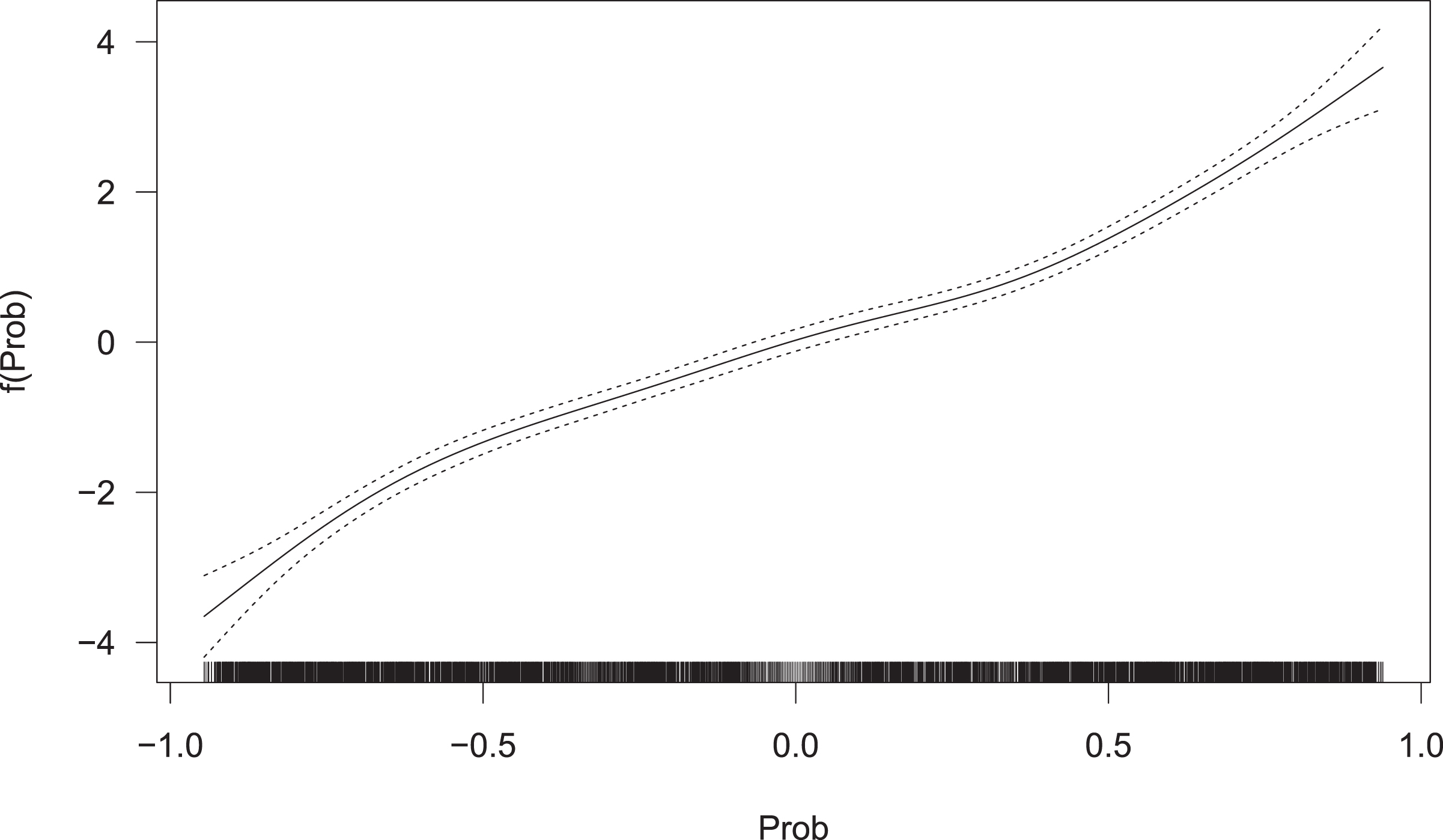
The assumption of linear effects can possibly be very limiting and lead to insufficient results. Therefore, spline models based on B-splines are also considered. Here, all 63 possible combinations are again compared with respect to various performance measures. To obtain smoothness, penalization of the splines is performed and, hence, P-splines are used. Furthermore, an additional regularization approach is used, i.e. an additional variable selection is performed on the spline effects. This is done by setting the spline coefficients to zero and is implemented in the gam-function from mgcv (Wood, 2017) via setting the select argument to TRUE. For the underlying methodology of this additional penalization and variable selection approach, see e.g. Marra and Wood (2011). We will later on see that exemplarily the effect of the variable probs is non-linear for very low and high values (see Fig. 1), which also seems to be reasonable (see our explanation in Section 5).
Fig. 1
Estimated non-linear effect of the variable Prob.
Surface-specific player skills (LASSO)
Since tennis is played on different surfaces (grass, hard court and clay court) and these surfaces have specific characteristics, so that each surface is played differently, it is plausible to assume that not every player copes equally well on every surface. For example, the Spaniard Rafael Nadal is considered as the “king of clay”, as he has won 14 French Open titles on this surface. At the same time, however, he was “only” able to win the Wimbledon title twice, which is played on grass. In contrast, the Swiss Roger Federer has already won Wimbledon eight times, but the French Open only once. In order to take into account these specific features of players and surfaces, a corresponding factor variable is created. Technically, this requires effect coding. Actually, to the data set artificially columns are added, whose entries are either 0, 1 or –1. Each column represents a combination between a player and one of the corresponding surfaces, i.e. for each player there are a maximum of three such columns. If a player has not played on one of the three surface types, the corresponding columns are omitted. Each row consists of exactly one entry of –1 and 1, respectively, while all other entries of the row are 0. The entry 1 is in the column of the combination of the first player and the corresponding surface on which the match took place. Analogously, the entry –1 is in the column of the combination of the second player and the surface. For example, the line
As a result, a large number of new covariates is constructed, namely 1,024, which generally leads to an extremely large number of parameters being estimated and the associated estimators becoming unstable. Therefore, for this approach the logistic regression model is combined with LASSO regularization. The influences of all covariates is assumed to be linear here. Via the surface-specific player skill parameters, the model can detect when a player has won or lost more often than average on a surface.
Global player skills (LASSO)
Analogously, it can be argued that there are also players who overall perform even better or worse than the information of their covariate values would suggest, i.e. who have a generally great or substandard talent and are therefore more likely to be assessed as winners or losers. For this purpose, similar to the previous paragraph, a corresponding factor variable is created, again using effect coding. In this case, we add only one column per player. The added columns again only have the entries 0, 1 or –1, where the values 1 and –1 occur exactly once per row. In each row, the value 1 appears at the position belonging to the first-named player and the value –1 at the position belonging to the second-named player, all remaining entries are 0. The following exemplary row
indicates that Rafael Nadal played as the second named player against the first named player Roger Federer. The column for the player Novak Djokovic (as well as for all other players), for example, is then 0, since he did not play. Again, those global player-specific abilities are then added to the design matrix and used along with the covariates defined in Section 2. The columns are then appended to the already existing record.
Again, a large number of new covariates is constructed, namely 426, so again a large number of player-specific skill parameters has to be estimated. And, hence, again we extend the logistic regression model with LASSO penalization and assume linear covariate effects only.
Benchmark model
As a benchmark model for prediction, we solely use the probabilities (probs) calculated from the average odds of the different bookmakers included in the deuce package. The winning probabilities in the i-th match
4.2Performance measures
To compare the selection of regression models in terms of their predictive performance on new, unseen data, the following criteria are considered. First, use
Classification rate
The (mean) classification rate indicates how many matches on average are correctly predicted by a certain model. It is defined by
Predictive Bernoulli likelihood
The predictive Bernoulli likelihood is based on the predicted probability for the true outcome and for n predictions is defined as
Brier score
The Brier score is based on the squared distances between the predicted probability and the actual (binary) output from the i-th match. It is defined according to Brier (1950) as
Betting profit
Another way to compare the predictive quality of different models is the betting profit. Let oddi1 and oddi2 be the odds from a specific betting provider for a win of the first and second player in the i-th match, respectively. If one bets one monetary unit on a win of the respective player, the expected betting returns for the i-th match are given by
Principally, the bet should of course be placed on the match outcome with maximum positive expected return. If the return is not positive for either outcome, no bet is placed on the corresponding match. In this work, to calculate actual, realistic betting returns, the odds of the specific betting provider Bet365 are used, i.e. it is assumed that the bets are placed with this provider. The total betting return is then the sum of all betting returns across all matches.
4.3Leave-one-tournament-out cross validation
To evaluate the models, all Grand Slam tournaments from 2011 to 2021 are used, i.e. the tournaments that took place in 2022 are initially not considered and are used as external validation data later on. So, from each of the 11 years four tournaments are used. A 43-fold CV-type strategy is performed with these tournaments. The data set then still contains 4,720 of the original 5,013 matches. The following scheme is used:
1 From the 43 Grand Slam tournaments present in the data set, a training data set of 42 tournaments and a test data set of the remaining tournament are constructed.
2 Then, all regression models introduced above are fitted:
(a) For the models with linear influences, the function glm from the R package stats (R Core Team, 2022) is used. As described in Section 4.1, there are 63 such models, each using at most one of the three variables for age.
(b) For the calculation of the spline models the function gam from the R package mgcv (Wood, 2004) is used. Again, there are also 63 different models here.
(c) In order to be able to compute the two LASSO-penalized models, first the design matrices have to be constructed as described in Section 4.1. For a proper usage of the LASSO, then all columns of the design matrix of the training data need to be standardized. The function cv.glmnet from the R package glmnet (Friedman et al., 2010) is used to compute both models. For this, a 10-fold (inner) CV is first performed on the current training data to find the optimal λ which provides the minimum deviance. The corresponding LASSO model is used afterwards for prediction. 10-fold CV is also recommended in Friedman et al. (2010).
(d) For prediction based on average betting odds, the probabilities calculated from odds are used as predicted probabilities.
3 After fitting the respective model, for each match of the test data the probabilities that the first player wins are predicted.
4 Steps 1–3 are repeated until each of the 43 tournaments has served once as a test data set.
5 Finally, the predicted results are compared with the actual results and the performance measures defined in Section 4.2 are calculated.
Table 1
Results of the cross validation for the (at most) best five models per model class (best performing model in bold font). In brackets are the betting profits per match and the ratio of all matches in which a bet was placed
| Explanatory | Class. | Likeli- | Brier | Betting | Amount of | |
| variables | rate | hood | score | profit | bets | |
| Linear | Prob | 0.7772 | 0.6919 | 0.1549 | -128.8 (-0.05) | 2696 (57.1 %) |
| Points, Prob | 0.7772 | 0.6917 | 0.1549 | -99.9 (-0.04) | 2395 (50.7 %) | |
| Rank, Prob | 0.7776 | 0.6918 | 0.1550 | -110.9 (-0.04) | 2707 (57.3 %) | |
| Age, Prob | 0.7766 | 0.6918 | 0.1550 | -150.3 (-0.05) | 2716 (57.5 %) | |
| Rank, Points, Prob | 0.7772 | 0.6917 | 0.1550 | -104.3 (-0.04) | 2418 (51.2 %) | |
| Splines | Prob | 0.7764 | 0.6912 | 0.1546 | 113.7 (0.09) | 1170 (24.8 %) |
| Rank, Prob | 0.7764 | 0.6912 | 0.1546 | 113.7 (0.09) | 1170 (24.8 %) | |
| Points, Prob | 0.7764 | 0.6912 | 0.1547 | 101.3 (0.08) | 1298 (27.5 %) | |
| Rank, Points, Prob | 0.7764 | 0.6912 | 0.1547 | 101.8 (0.08) | 1299 (27.5 %) | |
| Elo, Prob | 0.7764 | 0.6911 | 0.1547 | 106.9 (0.09) | 1175 (24.9 %) | |
| LASSO | Surface specific | 0.7774 | 0.6816 | 0.1551 | -225.3 (-0.12) | 1891 (40.1 %) |
| General skills | 0.7770 | 0.6838 | 0.1551 | -199.3 (-0.10) | 2002 (42.4 %) | |
| Benchmark | 0.7772 | 0.6709 | 0.1555 | -311.4 (-0.23) | 1359 (28.8 %) |
The classification rate is slightly above 77% for all models (see 1st column). Differences between the models can only be seen at the third decimal. The linear regression model with both rank and probs as covariates here performs best with a value of 0.7776, i.e. this model predicts the correct outcome for 77.76% of the matches.
The values of the predictive Bernoulli likelihood (2nd column) differ somewhat more. It is noticeable that within one group of model approaches the likelihood is almost the same (differences are only seen in the fourth decimal). The average likelihood of the models with both linear and non-linear effects is slightly more than 0.69, i.e. the models predict the correct outcome with an average probability of about 69%. The two LASSO models are just below 0.69. It is noticeable that the benchmark model has the lowest likelihood, which is 0.6709. The average betting provider correctly predicts the outcome of a match with an average probability of 67.09%.
The differences across model groups in the Brier scores are rather small, similar to the classification rate. The models with non-linear effects perform best in this regard with Brier scores between 0.1546 and 0.1547. The models with linear effects produce slightly larger values, followed by the LASSO models. In the case of the Brier score, the benchmark model again performs worst with a value of 0.1555.
The betting returns are negative for all models except for the spline-based approaches, and here there are substantial differences between the various modeling approaches. If linear effects are assumed, the losses range from about 100 to 150 monetary units. For the spline models, gains are achieved which lie between about 101 and 114 monetary units. In particular, the model in which either only prob or prob and rank were included perform best with a gain of about 114 monetary units. The two models with LASSO perform even worse than the linear models, with a betting loss of almost 200 and 225 money units. Once again, the benchmark model performs worst with a loss of about 311 monetary units. This comparatively high loss is due to the fact that this model almost always bets on the underdog, but the underdog rarely wins. The betting profit must be seen in relation to the number of bets placed. Here, the tendency can be seen that models with a high betting loss have the tendency to bet more often. It is particularly noticeable that bets are placed much less frequently when using the non-linear models compared to the other models. It can therefore be assumed that these models are a little more conservative. This can also be seen from the betting returns per match (bet). In some cases, the corresponding losses are significantly lower than those of the other model approaches.
4.4External validation
To validate the models from above with respect to their predictive performance on new, unseen test data, the three best models from the groups of modeling approaches with linear and non-linear effects are used, as well as the two LASSO models and the benchmark model. For this purpose, the performance measures are calculated on the four Grand Slam tournaments 2022. The data set then contains 293 matches. The validation is performed using a “rolling window”-type approach, i.e. one of the remaining tournaments is used as the test data set in chronological order. The training data set then continues to be constantly updated and enlarged, this scheme can be explained as follows:
1 First, all tournaments prior to 2022 are used as the training data set and then the models are fitted in a way as it is described in the second step of the CV approach described in Section 4.3. With those, then predictions can be obtained for the 2022 Australian Open, as this is the first Grand Slam tournament of the year 2022.
2 The new training data set will then contain all tournaments up to and including the Australian Open 2022, on which the models are fitted again and predictions are made for the French Open 2022, the 2nd Grand Slam tournament of the year 2022.
3 Now the French Open 2022 is added to the training data set and the models are fitted again. This will then be used to predict Wimbledon 2022.
4 Then, the Wimbledon 2022 matches will be added to the training data set, and again, the models are fitted and predictions are made for the final Grand Slam tournament, the US Open 2022.
5 Finally, the predicted results for all four tournaments are compared with the actual results and the performance measures are calculated.
Table 2
Results of the external validation for the (at most) best three models per model class from Section 4.3 (best performing model in bold font). In brackets are the betting profits per match and the ratio of all matches in which a bet was placed
| Explanatory | Class. | Likeli- | Brier | Betting | Amount of | |
| variables | rate | hood | score | profit | bets | |
| Linear | Prob | 0.7816 | 0.7036 | 0.1419 | -21.6 (-0.11) | 197 (67.2 %) |
| Points, Prob | 0.7747 | 0.7027 | 0.1421 | -17.4 (-0.09) | 191 (65.2 %) | |
| Rank, Prob | 0.7816 | 0.7037 | 0.1418 | -20.5 (-0.01) | 198 (67.6 %) | |
| Splines | Prob | 0.7782 | 0.7031 | 0.1413 | 4.2 (0.03) | 121 (41.3 %) |
| Rank, Prob | 0.7782 | 0.7031 | 0.1413 | 4.2 (0.03) | 121 (41.3 %) | |
| Points, Prob | 0.7782 | 0.7033 | 0.1411 | -0.28 (-0.00) | 126 (43.0 %) | |
| LASSO | Surface specific | 0.7782 | 0.6934 | 0.1423 | -24.4 (-0.15) | 161 (54.9 %) |
| General skills | 0.7782 | 0.6969 | 0.1416 | -16.1 (-0.09) | 171 (58.4 %) | |
| Benchmark | 0.7816 | 0.6810 | 0.1441 | -39 (-1.00) | 39 (13.3 %) |
The classification rate is again above 77% for all models, and for some models even above 78% and, hence, slightly better compared to the classification rates from the CV-type strategy from above. The best value is 78.16% and is achieved by three models. It is striking here that now the benchmark model is among the best.
Similar trends as in Table 1 (cf. page 9) can be seen for the likelihood, although the results here are somewhat better. The linear models achieve the highest likelihood, where the model including the covariates Rank and Prob delivers the best value with 0.7037, only slightly behind are the models with non-linear effects (all between 0.7031 and 0.7033). The LASSO models yield an even slightly smaller likelihood. The benchmark model again performs worst.
The Brier score for all models is around 0.141–0.142. In Section 4.3, the values were slightly larger. The benchmark model again yields the largest, and thus worst value with 0.1441. The best value is achieved by the non-linear model including covariates Points and Prob (0.1411).
Looking at the results of betting returns, the larger part of the results are similar to those of Table 1. The LASSO models and the linear models yields the largest betting loss: approximately between 16 and 24 monetary units each, respectively. The models with non-linear effects again mostly yield profits (about four monetary units). However, here the benchmark model yields the largest loss with 39 monetary units.
Also in terms of the number of bets placed, the results from Table 1 are mostly confirmed. The linear models again bet most frequently (in almost every third match), the LASSO models bet second most frequently (in about half of the matches). If non-linear effects are included, betting is even less frequent (in about 40% of the cases), these models seem to be again the most conservative ones, but at a higher level, since the proportion of bets placed has increased for each of these three model approaches compared to the results from Section 4.3. The same applies to the betting returns per match, which is now 0.00 monetary units of loss in the worst case. It is noticeable that bets were placed much less frequently with the benchmark model than with all other models. This was not the case in Section 4.3. There, a bet was placed in 28.8% of the possible matches, while here the percentage is only 13.3%.
5Discussion
In Section 4.3, a leave-one-tournament-out CV-type approach was performed with the 43 Grand Slam tournaments from the years 2011–2021. Since the tournaments actually were played one after the other in time, the CV-type strategy in a certain sense resulted in the setting that the past was predicted with information from the future. Initially, this argues against the normal intuition of prediction, since, for example, players with currently high rankings are also more likely to have had high rankings in the past tournament, i.e. the values are correlated. However, since the crucial assumption that the yi|xi1, …, xip are (conditionally on the covariate information) independent for i = 1, …, n is still realistic, CV was used here as a technical tool to compare performance across many different prediction models.
Instead of a CV-type approach, a performance comparison over a continuously updating data set (“rolling window”) could be considered, as in Section 4.4. This would have the advantage that the temporal structure of the data could be preserved. However, the CV-type strategy here had the advantage that the models could be compared on more data. Thus, each tournament served once as a test data set and since this was only used for an initial comparison to find principally suitable models, CV was preferred to the rolling window approach.
For the models from Table 1 (page 9) and Table 2 (page 11) it is noticeable that the variable Prob is always selected. So the bookmaker information seems to be very important and to have a big influence on the prediction. This could also be a reason why the models all perform quite similarly. The number of ranking points or the rank itself are also partly selected in the three best linear and spline-based models. Hence, these variables also appear to be important to a certain extend, although not quite as influential as the odds.
It is hardly possible to filter out a clear winner amongst the regarded models, since they differ little with regard to the performance measures. If one initially compares only the three regression modeling approaches, tendencies can be identified. When considering the classification rate and predictive Bernoulli likelihood, the linear models might be very slightly preferred. Regarding the Brier score, the spline-based models perform slightly better.
However, since the two LASSO models never perform best with respect to any of the measures, and since also their respective betting loss is the largest, these models are rather not to be preferred. Within the first modeling approach, according to the results from Table 2 (page 11), the linear model with the ranking position and the betting odds is best suited to model a tennis match. Within the spline models, the model including only the betting odds and the number of ranking points could be chosen as the winner with respect to the first three performance measures. But as all three models almost yield equal results, also the most sparse and simple model, here the first one just including the betting odds, could be chosen, as it also results in positive betting returns. Between the two models selected in this way (Rank and Prob as linear effects or only Prob as a non-linear effect), the betting profit should also be considered. If this is taken into account, the spline model should be preferred; if the betting returns are not considered to be important, the linear model should be selected.
Spline models
Figure 1 shows the fitted spline of the variable Prob and its pointwise 95% confidence intervals. For this purpose, the model was fitted with the covariate Prob on all tournaments.
The estimated effect looks almost linear between -0.5 and 0.5, and then steeper at both edges. This suggests that betting providers use somewhat “unfair” or special odds in these regions. If the absolute difference in the winning probabilities is more than 0.5, it can be assumed that a strong player is playing against an extreme underdog, which occurs particularly often in the first round of a tournament. For example, the favorite in a match may have a 99% chance of winning the match according to the betting companies, while the underdog has a 1% chance of winning. This would result in odds of 1.01 for the favorite and 100 for the underdog (ignoring the bookmaker’s margin for a moment). However, since an underdog’s win is very unlikely, the bookmaker probably don’t always withhold the same margin from an underdog’s odds. For higher odds, they probably withdraw larger margins than for lower odds. Therefore, it seems reasonable to assume that the effect of Prob is not linear, but instead (slightly) non-linear.
LASSO models
In determining the optimal penalty strength λopt for the LASSO models, 10-fold CV was performed for a sequence of different λ values and the mean deviance was calculated. Figure 2 shows this process as an example with the 2011–2021 data for the model with general player skills.
Fig. 2
CV-deviance of LASSO-model as a function of λ; vertical dashed line: λopt.
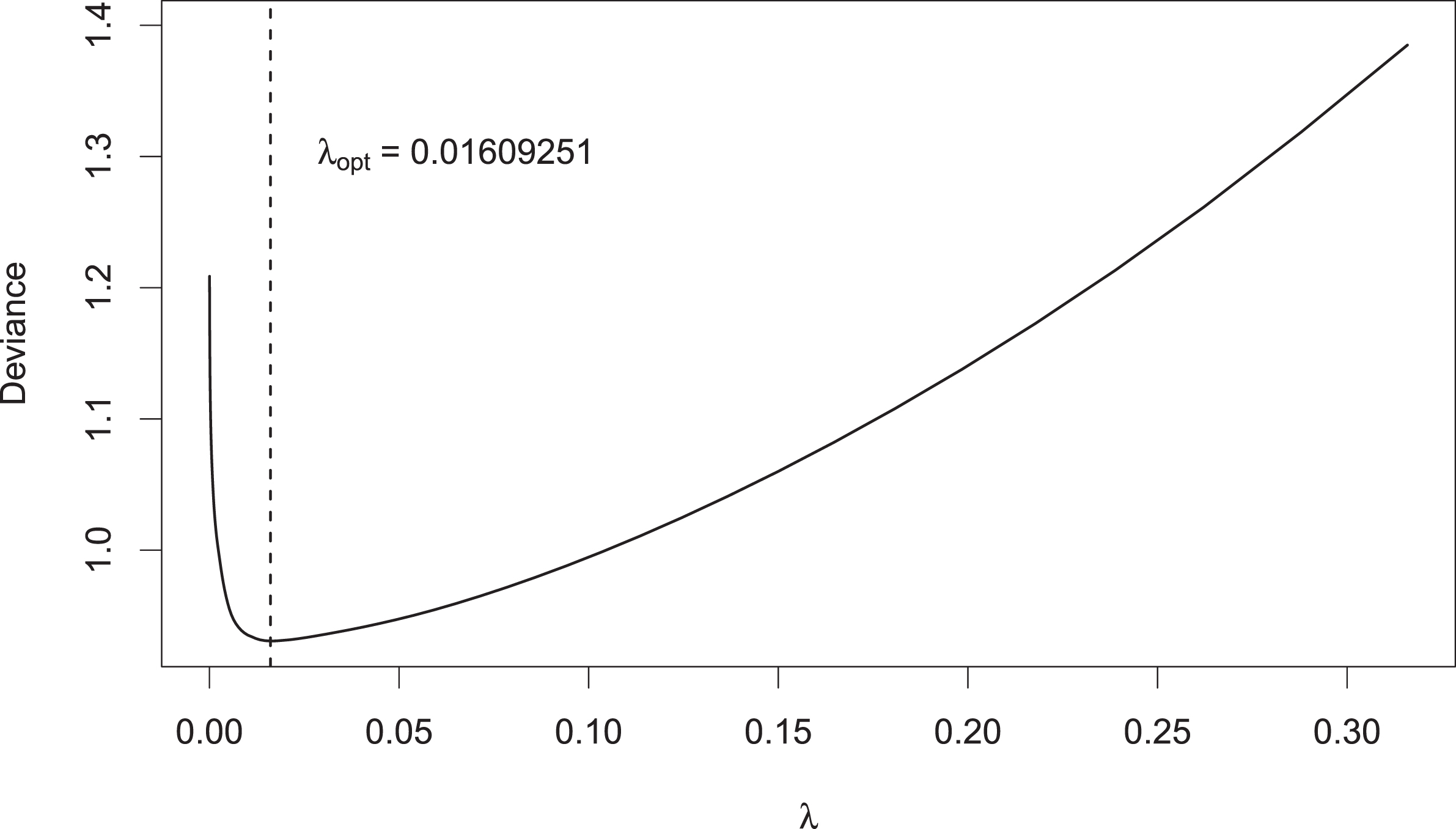
Here, λopt = 0.0161 provided a minimum deviance of 0.9504. The LASSO model with this choice for λopt was then used to predict the Australian Open 2022. For the same setting, Fig. 3 on page 13 shows the corresponding coefficient paths as a function of λ, together with λopt as the vertical dashed line.
Fig. 3
Coefficient paths vs. penalty strength λ; vertical dashed line: λopt.
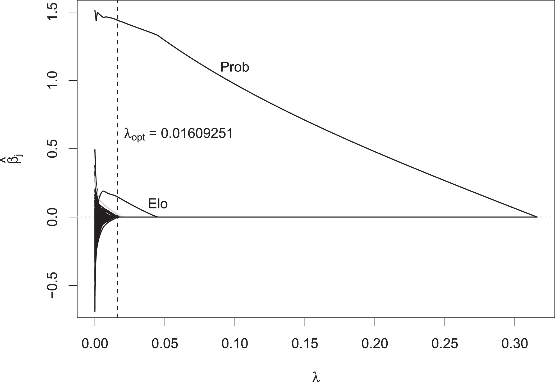
For any λ between about 0.02 and 0.3, every coefficient except that of the variable Prob is shrunk to zero. For decreasing λ, the coefficient of Prob becomes larger, again showing the importance of this variable. For λ smaller than 0.02, the coefficients of both variables Points and Elo are also positive. The coefficients estimated by the model can be read at the location of λopt. Prob has a coefficient estimate of 1.50, Points of 0.06 and Elo of 0.02. Among others, the coefficient estimate of the player Tennys Sandgren (plotted in gray), is also positive at this point with a value of 0.03.
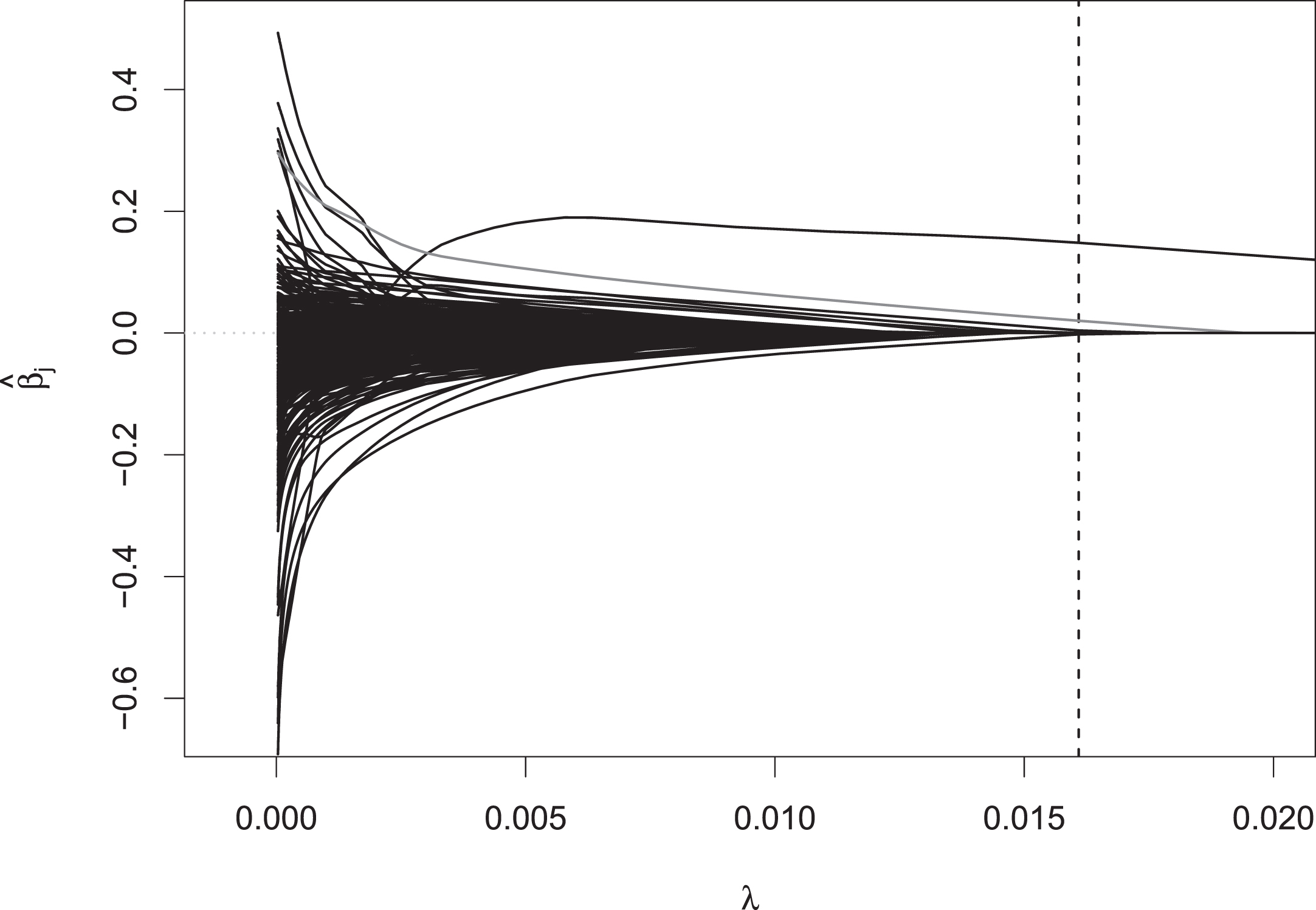
This can be seen in more detail in Fig. 4, where it is zoomed into the range of the smaller λ values. At the optimal amount of penalization, the coefficients of most other players are 0, except for ten different players. Among those, Tennys Sandgren has the largest estimated regression coefficient with a value of 0.03, so if he is one of the two players competing in a match, the value of 0.03 is added to his linear predictor for modeling the probability of him winning the match, so he seems to perform a bit better than his covariate values indicate. If one chooses λ to be even smaller, the coefficient estimates of many other players are also no longer shrunken to zero, and they are given positive or negative abilities. As the LASSO estimator for smaller λ gets closer and closer to the maximum likelihood estimator, these coefficient estimates are numerically very unstable. This can also be seen in the path of the variable Prob (see Fig. 3), which shows a very wiggly behavior for λ close to 0.
Fig. 4
Zoomed fragment of the coefficient paths for lower λ values.
6Summary and overview
In this work, tennis matches in Grand Slam tournaments were modeled within the framework of regression. For this purpose, a data set that was compiled using the R package deuce (Kovalchik, 2018). This contained information on 5,013 matches in men’s Grand Slam tournaments from the years 2011–2022. This included the age difference of both players (Age), the difference in their ranking positions (Rank) and ranking points (Points), in Elo numbers (Elo), in probabilities for the victory of the players, calculated from the average odds by the betting providers (Prob), as well as the two additional age variables Age.30 and Age.int, which should take into account that the optimal age of a tennis player is between 28 and 32 years.
Different regression approaches were considered for modeling and prediction of tennis matches. As there are only two possible outcomes in tennis (win or loss), all models were based on a binary outcome and, hence, on logistic regression, modeling the probability of the first named player to win. It was discussed that modeling with intercept would not be useful as this would incorporate a kind of home effect for the first named player –a property which was not desired here.
The different modeling approaches were compared in a 43-fold leave-one-tournament-out CV-type strategy. Each of the 43 Grand Slam tournaments from 2011 to 2021 served once as a test data set. The following models were included:
– Models with linear effects: to find suitable covariates, all possible combinations of the seven covariates were considered such that at most one of the three age variables was incorporated. This resulted in 63 models.
– Models with non-linear effects (splines): Again, 63 models were considered.
– A model which took into account surface- and player-specific effects. Due to the large amount of unknown parameters, here LASSO penalization was used.
– A model that considered general player-specific abilities. Again, LASSO penalization was used.
– A benchmark model, where the predicted probabilities were derived from average betting odds.
It was found that all models performed very similarly in terms of classification rate, likelihood and Brier score. The classification rate was slightly above 77% for all models, meaning that the models predicted the correct outcome in about 77% of the matches. The predictive Bernoulli likelihood was about 0.69 for both linear and non-linear models, while the LASSO models and the benchmark model were slightly below. The models thus predicted with an average probability of about 69% the correct outcome of a match. The Brier score was slightly above 0.15 for all models, differences were mostly found in the third decimal. When comparing the betting profits and the amount of bets placed, it was found that only the spline models achieved positive betting returns, but also placed fewer bets. Therefore, it can be assumed that these models are more conservative (and thus probably safer) in terms of betting.
The tournaments in 2022 were then used as an external validation data set. The three best models with each linear and non-linear effects, the two LASSO models and the benchmark model were then compared again. The results of the preceding CV-type competition could be mostly confirmed, with the values of the performance measures generally being slightly better than for the CV: the classification rate was around 0.775 - 0.782, the predictive likelihood yielded around 0.693 - 0.704 and the Brier score was between 0.141 - 0.142. With regard to the betting returns, again only the spline models achieved a betting profit, except for the model with the number of ranking points and the betting odds led to loss. The proportion of placed bets increased for all models, only the benchmark model placed considerably fewer bets than in the preceding CV-type competition. The most striking here was that, again the benchmark model was no better than the other models for most performance measures.
In a more detailed discussion, it was pointed out that the CV-type strategy here was preferable to a “rolling window approach” in finding models, since on the one hand the assumption of independence of the observations of the target variable, given the covariates, is fulfilled. Secondly, this allowed the models to be compared on more data, as the initial aim was to find suitable models. Furthermore, it was emphasized that the betting odds are very important for the prediction. In addition, it could be worked out that within the linear models the covariates Rank and Prob provided the best results. Within the spline approach, all three models provided almost equal results. Due to simplicity, the model that only considered betting odds would be preferred here. The LASSO models tended to perform worse than the other models and therefore could not really be recommended. The obtained betting returns can be used to decide between the first two types of approaches. They turned out to be positive for the best spline model, while the linear model yielded a loss. However, the classification rate and predictive likelihood were better for the latter model. It was also notable that all models performed at least as well as the benchmark model.
Lastly, the spline model with the Prob variable and the model with general player-specific skills were examined in more detail. Based on the corresponding fitted smooth effect, the behavior of the bookmakers in setting odds for an extreme underdog were discussed. Using the LASSO model for general player-specific skills, the CV for finding an optimal λ via deviance minimization was illustrated. In addition, the corresponding coefficient paths for the different covariates were shown and explained.
In future research, an upcoming complete tournament could also be repeatedly simulated, and then the probability of a certain player to win the tournament could be determined. This can take advantage of the fact that the tournament course is completely drawn before the start, i.e. it can already be said on the basis of the tournament tree that two players can meet at earliest in a certain round. This means that is not necessary to take into account whether someone has finished first or second in a certain group stage, as it is the case in soccer, for example. With such an approach, however, only the match-specific betting odds for the first round would be available. Models that do not use the odds as covariates could then be preferable, but this could lead to a poorer prediction performance due to the large influence of this variable. Alternatively, one could look at models that do not use the odds for individual matches, but instead use odds set before the tournament on each player to win the whole tournament.
Moreover, another extension of the approach proposed here would be to allow for more flexible, time-varying player-specific ability parameters, similar e.g. to the approach proposed by Ley et al. (2019) for modeling soccer. This approach has also been used successfully and the resulting estimates have been incorporated as a so-called “hybrid” feature in a random forest model for predicting the FIFA World Cup 2018 in Groll et al. (2019), and hence, seems to be also promising in tennis. And the authors have already planned to carry over this idea to tennis. To do so, a different (and much larger) data set has to be collected and also a separate, quite complex model specifically designed for historic match data has to be built up.
Finally, as already stated, in this work only (directly interpretable) approaches within the framework of regression were analyzed. In future research, we have planned to compare their performance with different complex machine learning models, which often have the capapbility to further increase the predictive performance, though coming with the substantial draw-back of loosing interpretability. For that reason, they typically should be equipped with certain methods of interpretable machine learning (IML), such as partial dependence plots Friedman, 2001, ICE plots Goldstein et al., 2015 and ALE plots Apley and Zhu, 2020. A first attempt to summarize the limited selection of available methods for interpretable ML appears in Molnar (2020).
References
1 | Apley D.W. , Zhu J. , Visualizing the effects of predictor variables in black box supervised learning models, Journal of the Royal Statistical Society Series B: Statistical Methodology 82: (4), 1059–1086. |
2 | Arcagni A. , Candila V. , Grassi R. 2022, A new model for predicting the winner in tennis based on the eigenvector centrality, Annals of Operations Research, pages 1-18. |
3 | Bayram F. , Garbarino D. , Barla A. 2021, Predicting tennis match outcomes with network analysis and machine learning, In International Conference on Current Trends in Theory and Practice of Informatics, pages 505-518. Springer. |
4 | Brier G.W. , Verification of forecasts expressed in terms of probability, Monthly Weather Review 78: , 1–3. |
5 | Chitnis A. , Vaidya O. , Performance assessment of tennis players: Application of dea, Procedia-Social and Behavioral Sciences 133: , 74–83. |
6 | Clarke S.R. , Dyte D. , Using official ratings to simulate major tennis tournaments, International Transactions in Operational Research 7: (6), 585–594. |
7 | Del Corral J. , Prieto-Rodrí guez J. , Are differences in ranks good predictors for grand slam tennis matches? International Journal of Forecasting 26: (3), 551–563. |
8 | Easton S. , Uylangco K. , Forecasting outcomes in tennis matches using within-match betting markets, International Journal of Forecasting 26: (3), 564–575. |
9 | Eilers P.H. , Marx B.D 2021, Practical smoothing: The joys of P-splines, Cambridge University Press. |
10 | Eilers P.H.C. , Marx B.D., , Flexible smoothing with B-splines and penalties, Statistical Science 11: , 89–121. |
11 | Fahrmeir L. , Kneib T. , Lang S. , Marx B. 2013, Regression, Modells, Methods and Applications, Springer, Berlin. |
12 | Fahrmeir L. , Tutz G 2001, Multivariate Statistical Modelling Based on Generalized Linear Models, Springer-Verlag, New York, 2nd edition. |
13 | Friedman J. , Hastie T. , Tibshirani R. Regularization paths for generalized linear models via coordinate descent, Journal of Statistical Software 33: (1), 1–22. |
14 | Friedman J.H. , Greedy function approximation: a gradient boosting machine, Annals of Statistics 29: , 337–407. |
15 | Goldstein A , Kapelner A. , Bleich J. , Pitkin E. , Peeking inside the black box: Visualizing statistical learning with plots of individual conditional expectation, Journal of Computational and Graphical Statistics 24: (1), 44–65. |
16 | Groll A. , Ley C. , Schauberger G. , Van Eetvelde H. A hybrid random forest to predict soccer matches in international tournaments, Journal of Quantitative Analysis in Sports 15: , 271–287. |
17 | Gu W. , Saaty T.L. , Predicting the outcome of a tennis tournament: Based on both data and judgments, Journal of Systems Science and Systems Engineering 28: (3), 317–343. |
18 | Klaassen F.J. , Magnus J.R. , Forecasting the winner of a tennis match, European Journal of Operational Research 148: (2), 257–267. |
19 | Kovalchik S. 2018, deuce: resources for analysis of professional tennis data, R package version, 1. |
20 | Lennartz J. , Groll A. , van der Wurp H. Predicting table tennis tournaments: A comparison of statistical modelling techniques, International Journal of Racket Sports Science 3: (2), 2021. |
21 | Ley C., , Wiele T.V.d. , Eetvelde H.V. Ranking soccer teams on the basis of their current strength: A comparison of maximum likelihood approaches, Statistical Modelling 19: (1), 55–73. |
22 | Ma S.C. , Ma S.M. , Wu J.H. , Rotherham I.D. , Host residents’ perception changes on major sport events, European Sport Management Quarterly 13: (5), 511–536. |
23 | Marra G. , Practical variable selection for generalized additive models, Computational Statistics & Data Analysis 55: (7), 2372–2387. |
24 | McHale I. , Morton A. , A bradley-terry type model for forecasting tennis match results, International Journal of Forecasting 27: (2), 619–630. |
25 | Molnar C. 2020, Interpretable machine learning, Lulu. com. |
26 | Nelder J.A. , Wedderburn R.W.M. , Generalized linear models, Journal of the Royal Statistical Society, A 135: , 370–384. |
27 | Park M.Y. , Hastie T. , L1-regularization path algorithm for generalized linear models, Journal of the Royal Statistical Society Series B 19: , 659–677. |
28 | R Core Team 2022, R: A Language and Environment for Statistical Computing, R Foundation for Statistical Computing, Vienna, Austria. |
29 | Radicchi F. , Who is the best player ever? a complex network analysis of the history of professional tennis, PloS One 6: (2), e17249. |
30 | Schauberger G. , Groll A. , Predicting matches in international football tournaments with random forests, Statistical Modelling 18: (5-6), 460–482. |
31 | Somboonphokkaphan A. , Phimoltares S. , Lursinsap C. 2009, Tennis winner prediction based on time-series history with neural modeling, In Proceedings of the International Multi Conference of Engineers and Computer Scientists, volume 1, pages 18-20. Citeseer, |
32 | Tibshirani R. , Regression shrinkage and selection via the Lasso, Journal of the Royal Statistical Society, B 58: , 267–288. |
33 | Weston D. 2014, Using age statistics to gain a tennis betting edge, http://www.pinnacle.com/en/betting-articles/Tennis/atpplayers-tipping-point/LMPJF7BY7BKR2EY |
34 | Whiteside D. , Cant O. , Connolly M. , Reid M. , Monitoring hitting load in tennis using inertial sensors and machine learning, International Journal of Sports Physiology and Performance 12: (9), 1212–1217. |
35 | Wilkens S. , Sports prediction and betting models in the machine learning age: The case of tennis, Journal of Sports Analytics 7: (2), 99–117. |
36 | Wood S.N. , Stable and efficient multiple smoothing parameter estimation for generalized additive models, Journal of the American Statistical Association 99: (467), 673–686. |
37 | Wood S.N. 2017, Generalized Additive Models: An Introduction with R. Chapman & Hall/CRC, London, 2nd edition, |
38 | Yue J.C. , Chou E.P. , Hsieh M.-H. , Hsiao L.-C. , A study of forecasting tennis matches via the glicko model, PloS One 17: (4), e0266838. |


