
Modelling the financial contribution of soccer players to their clubs
Abstract
This paper presents a framework for evaluating the financial consequences of player transfers as seen from a club’s perspective. To this end, an objective player rating model is designed based on players’ contribution towards creating a positive goals differential for their team. A regression model is then applied to predict match outcomes as a function of the players involved in a match. Finally, Monte Carlo simulation is used to predict the final league standings and the financial gains obtained as a function of sporting success. The framework is illustrated on player transfers from the 2014-2015 English Premier League season.
1Introduction
Soccer, or association football, is one of the largest sports in the world. The last two decades have seen the revenues of leading European association football clubs rising steadily, with broadcasting windfalls in particular soaring (Dobson and Goddard, 2001). While revenues soar, it appears that owners of European soccer clubs are in general not seeking to maximize profits; many clubs’ losses and debts are shown to be quite severe, while dividends are seldom paid out. Sloane (1971) presents alternative objectives such as maximising supporter attendances or sporting success, while the clubs’ financial security must be maintained.
Assuming maximisation of wins rather than profit, competitive balance in league competition is strengthened by increased sharing of central revenue (Sloane, 2015). In 2007, the top five clubs in England and Spain received about half and two thirds of all broadcast revenue, respectively (Vrooman, 2007). Szymanski and Zimbalist (2005) comment that while North American sports such as baseball or American football remain closed competitions with exclusive franchise rights, they remain more profitable than European sports leagues practising promotion and relegation. Salary caps, player drafts, and roster limits are restrictions that remain almost exclusive to North American sports (Sloane, 2015). Meanwhile, in European soccer, while limits on squad size are also coming into effect in several competitions, players are still routinely traded as part of big-money deals negotiated by clubs with typically very little interference. American sports and their clubs are therefore seen as more receptive of the idea of profit maximisation and economic rationality (Sloane, 2015). However, with an increased competitive balance, resulting from a more even income through broadcast revenue, English soccer clubs may get a competitive advantage from using better tools to assess the economic consequences of player trades.
This paper presents a framework for evaluating player transfers in European soccer leagues, using illustrative examples from the English Premier League. Gerrard (2014) discussed two types of player valuation in soccer. First, comparative valuation is based on using observable market values from recent transactions to form an anchor that is then adjusted based on the particular player evaluated. For soccer, this has been explored using multiple linear regression. Frick (2007) summarized early work, which uses ordinary least squares regression to find variables that describe observed transfer fees. Typical significant independent variables include age, international caps, career games played, goals scored, and attributes of the buying and selling clubs. More recently, Sæbø and Hvattum (2015) found that a simple, objective player rating can explain a large portion of the variance in observed transfer fees, with additional significant factors including age, nationality, international caps, and the remaining contract time. Ruijg and van Ophem(2015) presented an estimation method to correct for sample selectivity, finding that the most important determinants for making a good transfer are age, average number of minutes played, and not being a goal keeper.
Herm et al. (2014) examined the ability of an online community to assess players’ market values. A real option pricing framework for valuating players was derived by Tunaru et al. (2005) and later used in (Tunaru and Viney, 2010), highlighting that there is a difference in the value of a soccer player for their current club and for potential new clubs. The valuation framework is based on an analysis firm’s performance rating system for individual players, the Opta Index, with each player’s performance rating acting as the underlying asset in option price modelling. While the proposed valuation system does look at players’ value as a function of their performance, it does not consider club performances and direct player contributions to such. No definitions of relevant player contributions to results are offered, the Opta Index being assumed as a sufficient measure of player quality instead.
The second type of valuation discussed by Gerrard (2014) is fundamental valuation, which involves calculating the net benefits that the holder of an asset can expect to obtain. Regarding soccer players, this includes merit payments obtained through sporting performance and revenues based on a players image value. Pioneering work was done by Scully (1974) in the context of baseball: a team revenue equation based on player performance statistics fed into a team performance function to determine players marginal revenue contribution. Gerrard (2014) argues that it may be difficult to use a similar scheme for soccer, as baseball is a simple atomistic sport with a high degree of separability in player contributions, whereas soccer is a complex sport with a hierarchical dependence of player actions.
The first contribution of this paper is to present a coherent framework for valuing players in the context of specific clubs, so that clubs can evaluate player transfers based on their own performance and needs rather than relying on market mechanisms to price players. That is, we show that fundamental valuation of players is possible in the dynamic and fluid sport of soccer. As a second contribution, we present an improved top-down player rating system to assess the contribution of single players to the performance of a team as a whole. Third, we present an extensive computational study, including calculations for several cases of transfers to clubs in the English Premier League for the 2014-2015 season.
In the next section we describe the proposed framework for evaluating player transfers from a club perspective. The framework is based on the presence of objective player ratings, which can be used as input to model match outcome probabilities, which in turn are used in simulation of relevant competitions. Then, the framework is used to illustrate several transfers involving clubs in the English Premier League, estimating the economic consequences for the clubs involved. Concluding remarks are provided in the last section of the paper.
2Evaluation framework
The following presents a framework to estimate the influence a single player has on the sporting performance of a club. Assuming that the economic performance is related to the sporting performance, the framework can indicate how much a club should be willing to spend to secure the services of the given player. The framework has three components: 1) an evaluation of each player in terms of how they contribute to sporting success, 2) a prediction of outcomes of future matches based on the players involved, and 3) a prediction of competition results based on the ability to predict matches based on player evaluations. Limitations of the framework are discussed in the concluding remarks of the paper.
2.1Player ratings
The first building block of the framework consists of evaluating the active soccer players. While there has been some work on methods for rating and ranking soccer teams (Constantinou and Fenton., 2013; Hvattum and Arntzen, 2010; Lasek et al., 2013), the evaluation of players has received much less attention. Sæbø and Hvattum (2015) proposed a top-down rating model for soccer players, using a regression model capturing the performance of players relative to their team mates and the opposition. The model was based on similar models, referred to as adjusted plus-minus ratings, from basketball (Winston, 2009) and ice hockey (Macdonald, 2011, 2012). McHale et al. (2012) describe a rating for soccer players based on six subindices, the first of which uses a bottom-up approach to estimate the contribution of players to match outcomes, whereas the other five are based on the number of minutes played (in two different ways), the number of goals scored, the number of assists, and the number of clean sheets. The final rating is a weighted sum of the six subindices. The rating proposed by McHale et al. (2012) requires more detailed data than the plus-minus ratings that we describe and extend in the following.
A plus-minus rating measures the number of goals scored minus the number of goals conceded when a given player is in action. In its purest form, it ignores the quality of the opposition and the number of minutes played. The adjusted plus-minus rating was first proposed for basketball players (Winston, 2009). In the context of soccer, consider a set of past matches. Each match is divided into a set of segments, where each segment corresponds to a period of time where the set of players on the pitch is constant. Considering a maximum of three substitutions per team and some players being sent off, a match consists of just over six segments on average. For each segment i, define
and let yi = Hi - Ai, where Hi is the home goals scored and Ai is the away goals scored within the segment. Each player j is then assigned a rating βj that describes the player’s relative contribution towards the goals differential, given by
(1)
where ɛ is a column vector of error terms, as otherwise the resulting equation is unlikely to have any solutions whenever ratings are calculated based on a large set of historical match data. Ratings can thus be found by using ordinary least squares regression to minimize the model errors, given as the sum of squared differences between the actual goals differences, y, and the model predictions
The regularized adjusted plus-minus rating proposed by Sæbø and Hvattum (2015) includes the following modifications: First, the duration in minutes, Di, of different segments may vary significantly. Ratings are therefore interpreted as the marginal contribution of a player to the goal difference of the whole team per 90 minutes, and the goal differences, yi, are scaled accordingly. The possibility of having time-varying scoring rates in a match is not taken into account. Second, to represent the home field advantage, an extra home dummy player is instantiated – a contributor to results that will be included in every home team’s starting lineup. Third, a football match is affected by the showing of red cards and a similar solution as for home advantage is used: four dismissal dummy variables are instantiated. Whenever a team is shown their first red card, the player in question is replaced by the “first dismissal” dummy player. A second dismissal leads to the substitution of the offending player for a “second dismissal” dummy, and so forth. When a dismissal is cancelled out, that is, a team loses one of its surplus players, the relevant dismissal dummy is dismissed. Forth, all past observations of performances are not weighted identically. Similar to what was done by (Dixon and Coles, 1997), all past observations are down-weighted exponentially, depending on the age of the observations in number of years, t, and a discounting parameter, k. This discounting of older observations means greater emphasis is placed on recent performances. Furthermore, this allows dynamic ratings that change more quickly, staying in tune with recent trends. By setting k = 0, the model allows all observations to have equal weight, as in the original plus-minus ratings.
Closer inspection of the ratings produced according to Sæbø and Hvattum (2015) revealed that the model did not sufficiently differentiate between players from different divisions or different league systems. A new extension is therefore considered, where a factor depending on the players’ current league and division (hereafter referred to as a tournament) is added. Letting N be the number of players and B be the number of tournaments, there will be a total of N + B + 5 variables: one for each player, one for each tournament, one for the home field advantage, and four for red card dummy players. For a segment i, let nij be 1 if player j plays for the home team in the segment, -1 if player j plays for the away team, and 0 otherwise. Similarly, let mij be the number of home team players minus the number of away team players, considering only players whose most recent match was in tournament j. Let rij be 1 if the home team has received at least j red cards and the away team has not, -1 if the away team has received at least j red cards and the home team has not, and 0 otherwise. Let qi be equal to 1 if the match involves a home field advantage, and 0 if the match is played on neutral ground. Each segment i corresponds to one row of the x matrix and one value in y as follows:
For player j and tournament b, let fjb be 1 if player j has played in tournament b and has not played in any other tournament afterwards, and let fjb be 0 otherwise. The final rating of player j, pj, can then be expressed as
(2)
where
(3)
and I is the identity matrix and λ is a parameter that signifies the strictness of the regularization. Setting λ = 0 reduces Equation (3) to an ordinary least squares problem, while increasing the parameter λ means some information is sacrificed in an attempt to tackle noise in the data.
To illustrate the player rating model, consider the following, simplified example. A single match is played between two teams each fielding only three players at any time. The home team comprises players 1–4, and the away team comprises players 5–8. The match starts with players 1–3 and 5–7 on the field. The home team scores three goals, after 21, 41, and 87 minutes, respectively. The away team scores one goal, after 67 minutes. After 45 minutes, player 2 is substituted with player 4, and after 84 minutes, player 5 is substituted with player 8. A red card is given to player 7 after 72 minutes. All players have had their last appearance in the same tournament (b = 1), except player 4, who now plays in a different tournament (b = 2). Time is not discounted, using k = 0. This results in the following rating model:
Columns 1–8 correspond to the players’ individual rating component, columns 9 and 10 are related to the estimation of the tournament rating component, the next four columns are for red cards, and column 15 is for the home advantage. The first row corresponds to minutes 1–45, the second row minutes 46–72, the third row minutes 73–84, and the fourth row minutes 85–90. The model is solved using Equation (3), and player ratings derived according to Equation (2). Figure (1) illustrates the resulting player ratings for different values of λ. As the home team won the match 3 to 1, the home team players are rated higher than the away team players. As not all players contributed in all segments, the model suggests to differentiate between the ratings of players on the same team, according to the results obtained in the particular segments where each player was present.
Fig.1
Ratings from an illustrative example with eight players.
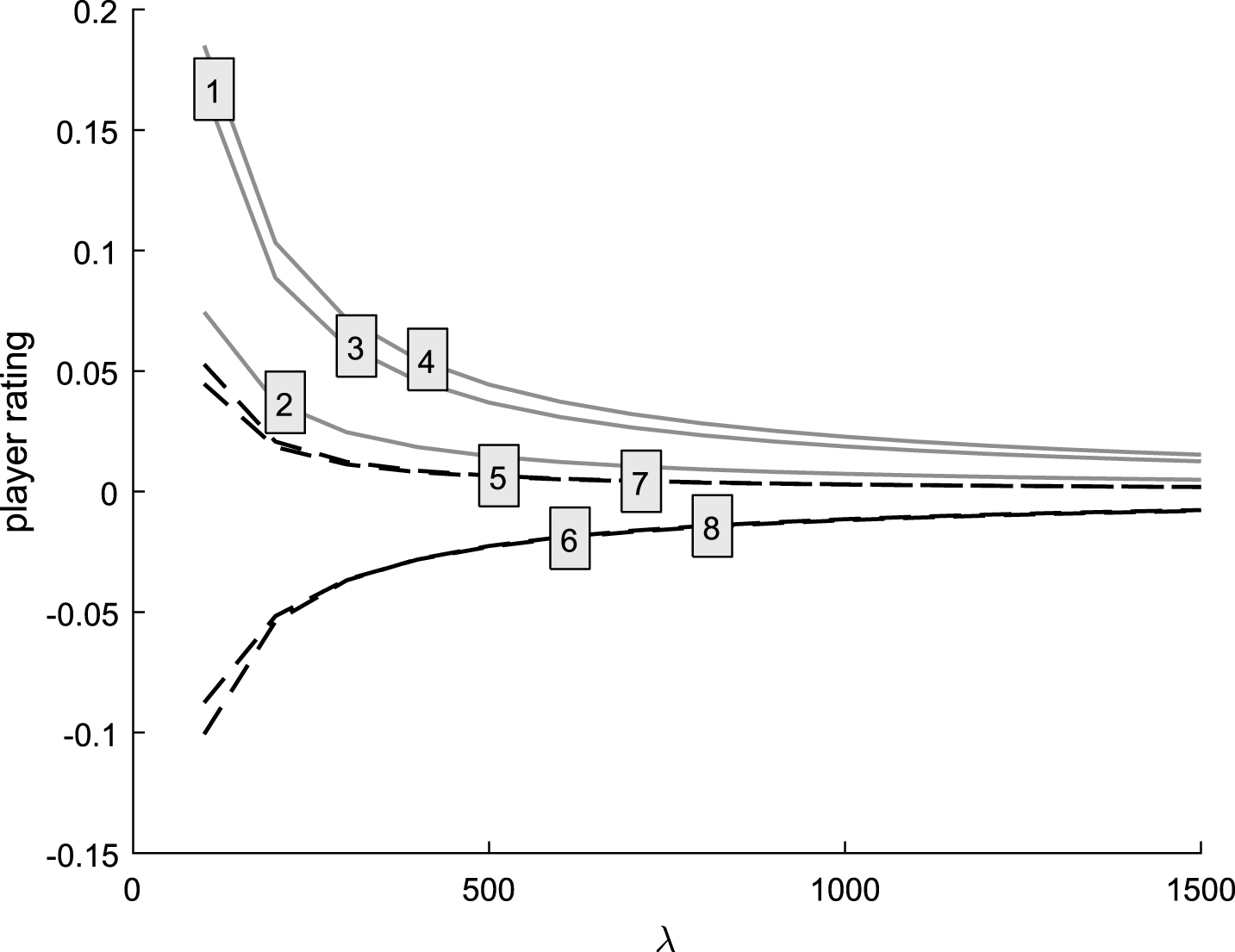
The resulting player ratings pj have several attractive features. The ratings take into account the score of every segment of soccer matches where a player has participated. A player’s rating depends on all other players involved in each segment: when the opposition has lower ratings, the players on a team must consistently obtain positive scores to maintain a difference in rating. If a team is consistently obtaining worse scores when a particular player is included, that player will be assigned a lower rating than the team mates. Players that appear in different leagues or divisions help to calibrate the rating levels in those competitions, to form an opinion on the difference in the average level of player quality. However, the player ratings are not a direct measure of player abilities, but rather of the relative performance in matches subject to whether or not a particular player is fielded.
It is often highlighted that two drawbacks of player rating models based on plus-minus ratings are 1) the collinearity resulting from some players almost always playing side by side, and 2) the fact that players with few minutes recorded have large standard errors. However, by using several seasons of data, the collinearity of players having overlapping playing time is merely theoretical: in modern soccer top teams rotate heavily on their starting lineups, and frequently rest top players in less important matches due to the tight playing schedule. Furthermore, by using the aforementioned regularization technique, players with few minutes are treated merely as average players in the particular tournament in which they have played. Using the framework to value players require them to have many minutes of recorded playing time, but the result is not influenced significantly by observing many other players with few minutes played.
2.2Prediction of match outcomes
The research literature has presented several methods for predicting outcomes of soccer matches, and detailed discussions regarding these methods can be found in (Constantinou et al., 2012; Goddard, 2005; Hvattum and Arntzen, 2010). In this paper, an ordered probit regression model is used for the prediction of match outcomes. A single independent variable is included, calculated as the difference of the average plus-minus rating for the home team players and the average plus-minus rating for the away team players. Only the players in the starting lineups are used when calculating the independent variable. The most recent plus-minus ratings, prior to a match, are used to calculate the independent variable, and players with no prior rating are excluded when taking the average rating. The model estimates three parameters: θ1, θ2, and γ, such that the probability of home wins, draws, and away wins can be stated as a function of the independent variable yOPR as follows:
where Φ is the cumulative distribution function of the standard normal distribution, and parameters are determined using maximum likelihood estimation.
2.3Simulation of competitions
With the ability to calculate player ratings, and a model that can be used to estimate probabilities for home wins, draws, and away wins based on those player ratings, entire league competitions can be simulated. Hvattum (2013) showed that Monte Carlo simulations of the top national leagues in Europe could produce league winner predictions matching those of the betting market. In that work, match outcome probabilities were calculated using ordered logit regression based on a single independent variable based on Elo ratings. Research on the use of ratings or ranks to predict cups for national teams has so far been outperformed by bookmaker odds (Min et al., 2008; Leitner et al., 2009).
Taking player ratings into consideration in the simulation of a competition requires additional input regarding team squads, and a model for team selection. We assume that all teams have a fixed squad from which to select players. For example, in the English Premier League, teams can register up to 25 senior players to be used between transfer windows. When simulating a whole season, player availability is uncertain, for example due to injuries and suspensions, and the team will typically use different players in the starting lineup in consecutive games. To capture the benefits of squad depth and take into consideration injuries, the simulation should not rely on a deterministic strategy, such as selecting the eleven most highly rated players as the starting lineup. Team selection must also respect the tactical challenges of professional football. Selecting players with no thought offered to their best positions on the pitch will leave a team open to exploitation by the opposition. For instance, no team would willingly select a goalkeeper to play in an outfield position.
Due consideration is given to the concerns above, and the following team selection algorithm is implemented: every player has a 0.10 chance of being unavailable for any given fixture. If possible, a team must be composed of exactly one goalkeeper and at least three defenders, three midfielders, and one forward. The best available players are selected for these eight positions. Finally, the next most highly rated players are selected so that the team counts eleven players. However, these players must not be goalkeepers and they must available (each with probability 0.90). All ratings (players, home advantage, and red cards) are taken as constant from the start of the season until the end. No consideration to the simulated results’ implied effect on the evolution of performance standards is given. That is, the simulation disregards the potential for streaks of bad form, the effect of the playing schedule, and the effect of matches being important for one team but not the opponent.
Each match is evaluated separately, and teams rewarded with three, one, or no points according to the result. Every point goes towards a regular league table, where all the teams and points totals are monitored. At the end of the season, all teams are rewarded with a conservative estimate of guaranteed financial revenue based on their position in the league table. Seeing as there is a lot of chance involved in the simulation of one season, the Monte Carlo simulation is repeated 100,000 times, and the average financial revenue is recorded for each club.
3Examples of using the framework
We now show how the framework can be used to evaluate player contributions in the English Premier League during the 2014-2015 season. We first describe the data used in the experiments. Then we describe the tuning of parameters for the plus-minus rating and the resulting ratings and the match outcome prediction model. Finally, we simulate the 2014-2015 season, illustrating the effect of some example player transfers.
3.1Data
Data for matches include the date of the match, the teams playing, the venue, and the competition. To calculate player ratings, detailed information must be present specifying the starting lineups, the time of substitutions and which players are involved, the time of red cards and which players are involved, and the time of goals scored. These data have been collected from the 2009-2010 season to the 2014-2015 season for the following national competitions: the English Premier League, the English Championship, the English FA Cup, the English League Cup, the German Bundesliga, the Italian Serie A, the French Ligue 1, the Spanish Primera División, the Portuguese Primeria Liga, the Dutch Eredivisie, the Belgian Pro League, and the Norwegian Tippeliga. In addition, European fixtures are included from the same time span for the UEFA Champions League and the UEFA Europa League.
The match data is used for different purposes. Matches played up to July 1 2010 are only used to calculate initial player ratings. Parameters for the player rating are tuned by maximizing the ability to predict match outcomes for matches played between July 1 2010 and July 1 2014. This is explained in the next subsection. Matches from July 1 2010 to July 1 2014 are then used to build the final match outcome prediction model. The matches played in the 2014-2015 season are only used, in addition to older games, to calculate the final player ratings, which are not used in any calculations. Although some matches are missing from the data set, in particular some early rounds of the national cups, there are in total 26,039 matches with sufficient data. The total number of players is 24,745, out of which 5,050 were active in at least one match during 2015.
The English Premier League’s revenue has risen quite significantly since its inception in 1992. Broadcasting revenue in particular has increased at a sharp rate. Central league revenue is distributed to each of the 20 clubs according to a set of rules (Harris, 2014). For the 2014-2015 season in question, each club received an equal share of GBP 52.2 million. Another sum, dependent on the final league position, came on top of that, adjusted linearly from GBP1.24 million for finishing last to 20 times that, GBP24.8 million, for winning the league. Finally, a fee is distributed according to how many club fixtures had been selected for live, domestic TV coverage. Every club is guaranteed a payment corresponding to ten live fixtures plus weekly highlights, GBP8.6 million. However, some teams who were broadcast well over 20 times received approximately GBP20 million.
Clubs that are relegated from the Premier League are also promised a guaranteed parachute payment, paid in yearly instalments, to help the clubs adjust to a competition with vastly inferior central revenue. The clubs which ended up relegated at the end of 2014-2015 were promised a total payment of GBP62.8 million. Meanwhile, at the top of the table, clubs compete for entry to European tournaments. These competitions, governed by UEFA, also promise significant revenue for the clubs involved. In the UEFA Champions League, every club that qualifies for the group stage is promised EUR8.6 million. However, the most significant revenues from the competition comes from broadcasting rights sales. The official numbers released following the 2012-2013 UEFA Champions League competition show that every English club participating received more than EUR15 million in broadcasting revenues. In addition, prize money is paid for group stage wins, as well as knockout stage wins. The top three English teams qualify directly to the Champions League group stage, while a fourth team plays two qualifying fixtures home and away against a foreign opposition team. Since 2004, only Everton, in 2005, have failed to proceed to the group stage from qualification. Meanwhile, the UEFA Europa League offers more modest fiscal rewards. Group stage participation only guarantees EUR1.3 million, however no English teams qualify directly to this stage.
In this simulation exercise, we do not speculate in popularity or broadcasters’ preferences, and so the most conservative revenue estimates are used as clubs’ financial returns on the competition. Also, the European competitions are not modelled, and so performance dependent revenues are ignored. An exception is made for UEFA Champions League group stage broadcasting revenue, which is assumed to reach a level of at least EUR15 million for each English team involved. The fourth placed Premier League team is conservatively assigned a 0.75 chance of qualifying to the group stage, and an exchange rate of 0.872 from 1 August 2013 is used to convert Euro revenues into Pound Sterling. UEFA Europa League revenue is ignored, as the expected revenue is low compared to both Champions League and Premier League revenue components. Clubs that are relegated (in 18th through 20th position) are allocated an additional return of one undiscounted total of parachute payments. The remaining 17 clubs, however, are assigned an additional guaranteed return equal to the value of finishing last in the next season. While relegated clubs are rewarded with a parachute payment, the much higher value of actually remaining in the competition and securing a place between 1st and 20th next season must be attributed to the remaining 17 clubs. The above conditions lead to the conservative estimate of the value of finishing in each of the Premier League’s 20 positions detailed in Table 1.
Table 1
Conservative estimate of guaranteed financial returns in the 2014-2015 Premier League
| Final position | Revenue [GBP million] |
| 1 | 234.02 |
| 2 | 232.78 |
| 3 | 231.54 |
| 4 | 225.15 |
| 5 | 205.48 |
| 6 | 204.24 |
| 7 | 203.00 |
| 8 | 201.76 |
| 9 | 200.52 |
| 10 | 199.28 |
| 11 | 198.04 |
| 12 | 196.80 |
| 13 | 195.56 |
| 14 | 194.32 |
| 15 | 193.08 |
| 16 | 191.84 |
| 17 | 190.60 |
| 18 | 127.32 |
| 19 | 126.08 |
| 20 | 124.84 |
3.2Calibration of models
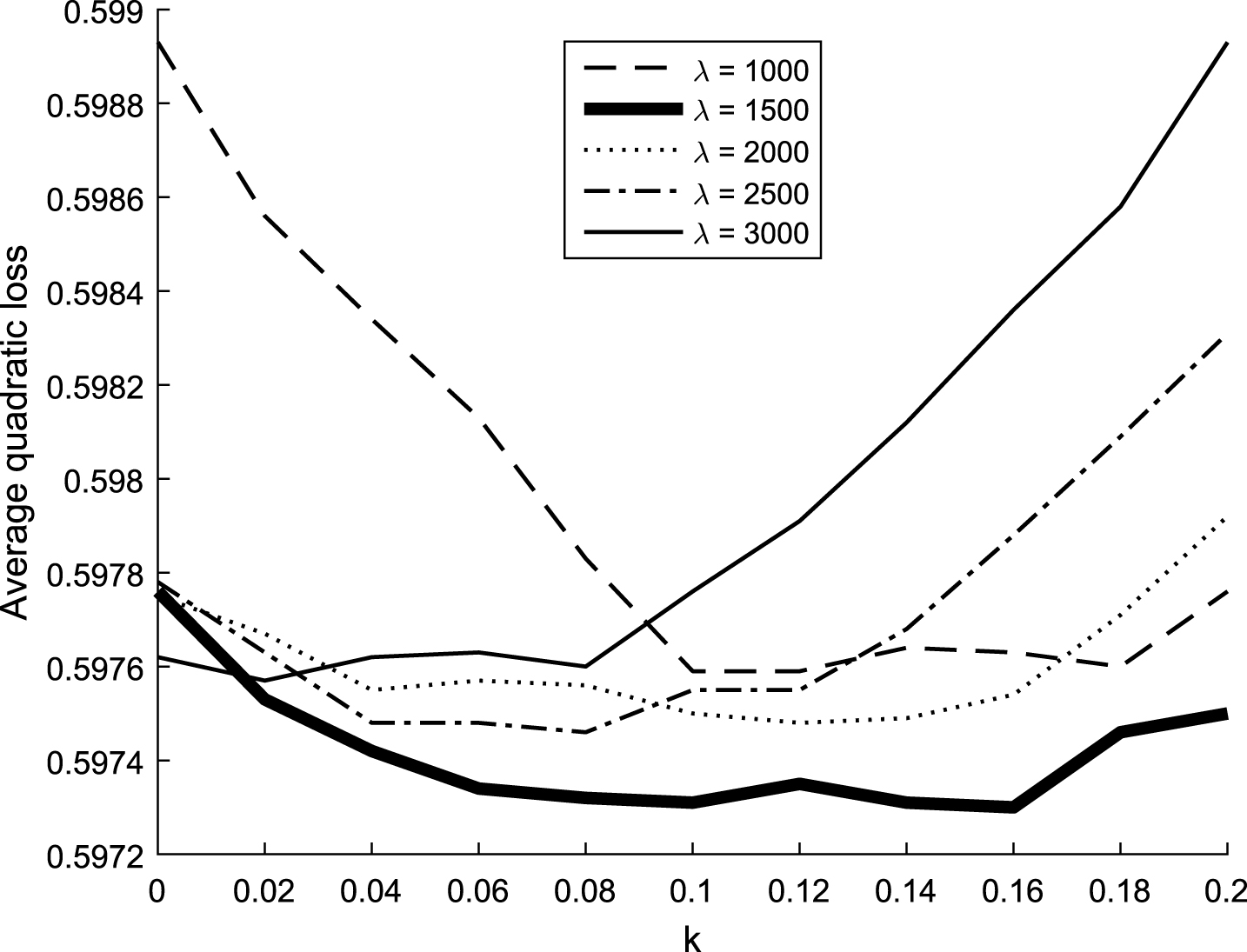
To determine suitable parameters, k and λ, for the player rating model, their ability to predict future match outcomes was used as a criterion. After calculating ratings, a prediction model was built on observations from June 1 of 2010 until the day before each predicted match. The prediction model was then used to predict the outcomes of 4,471 matches from the 2013-2014 season, providing a probability for each outcome. The quadratic loss (Witten and Frank, 2005) of the predictions was then calculated, and the average quadratic loss used to discriminate between the predictive ability of the ratings for each combination of parameter settings. The best parameters for the previous adjusted plus-minus rating model of (Sæbø and Hvattum, 2015), on the same set of matches, were k = 0.02 and λ = 3500, giving a quadratic loss of 0.5979. The best settings for the new rating model are k = 0.10 and λ = 1500, giving a quadratic loss of 0.5973. Figure 2 illustrates the tuning results for the new model.
Fig.2
Results from tuning parameters of the adjusted plus-minus rating model.
The complete data set, comprising 24,745 players and 26,039 matches, gives rise to a player rating model with 24,760 columns and 162,311 rows (segments). Using the final model parameters and the whole data set, the following rating values are obtained. The home field advantage is estimated to 0.388 per 90 minutes, as given by βj for j = N + B + 5. Regarding dismissals, the effect of the first red card is estimated to 1.53 goals per 90 minutes, whereas additional dismissals are attributed a much smaller effect, with 0.41 and 0.02 goals per 90 minutes, for the second and third dismissal, respectively. This may make sense, as being shown a first red card is often the time when tactics and preparations become distorted. Further reductions should have an added negative effect, but second and third dismissals are very likely to occur late on in games, with an increased likelihood that the result is more or less settled already. Furthermore, second and third dismissals are relatively rare, and the estimation is therefore distorted by the regularization coefficient of the regression.
Table 2 shows the estimated rating differences for different tournaments. Players only appearing in European competitions or English cups are implicitly given a tournament-rating component equal to 0. In Table 3, the 20 most highest rated active players on July 1 2015 are listed. The top list has players from all positions (goal keepers, defenders, midfielders, and forwards), from ages 23 to 36, from eight different clubs, and with 12 different nationalities. While subjective opinions may exist that a given player ought to be higher (or lower) in this list, it can be argued that the list seems to include predominantly good players, given that it is based solely on starting line-ups, goals, substitutions, and red cards recorded in 26,039 soccer matches between 2009 and 2015.
Table 2
Values for the tournaments, as given by βj for j = N + 1, …, N + B, following the end of the 2014-2015 season. The European competitions and the English cups were not included among the B tournaments
| League and division | Rating |
| English Premier League | 0.236 |
| German Bundesliga | 0.189 |
| Spanish Primera División | 0.179 |
| Italian Serie A | 0.178 |
| French Ligue 1 | 0.112 |
| English Championship | 0.090 |
| Portuguese Primeira Liga | 0.064 |
| Dutch Eredivisie | 0.030 |
| Belgian Pro League | 0.020 |
| Norwegian Tippeliga | 0.014 |
Table 3
The top 20 highest rated players on July 1 2015, out of 5,050 players with matches recorded in the last 12 months
| Rank | Name | Nationality | Team | Position | Year of birth | Minutes played | Rating |
| 1 | Lionel Messi | ARG | Barcelona | F | 1987 | 22973 | 0.519 |
| 2 | R. Lewandowski | POL | Bayern Munich | F | 1988 | 16316 | 0.514 |
| 3 | Marin Demichelis | ARG | Man. City | DM | 1980 | 17455 | 0.474 |
| 4 | Xabier Alonso | ESP | Bayern Munich | M | 1981 | 19493 | 0.463 |
| 5 | Marcelo | BRA | Real Madrid | DM | 1988 | 17821 | 0.448 |
| 6 | Olivier Giroud | FRA | Arsenal | F | 1986 | 16111 | 0.446 |
| 7 | Sergio Ramos | ESP | Real Madrid | D | 1986 | 20371 | 0.441 |
| 8 | Jesùs Navas | ESP | Man. City | MF | 1985 | 17626 | 0.433 |
| 9 | Manuel Neuer | GER | Bayern Munich | G | 1986 | 23494 | 0.431 |
| 10 | Arjen Robben | NED | Bayern Munich | F | 1984 | 12727 | 0.430 |
| 11 | Franck Ribèry | FRA | Bayern Munich | F | 1983 | 14449 | 0.430 |
| 12 | Cesc Fàbregas | ESP | Chelsea | MF | 1987 | 18107 | 0.429 |
| 13 | Cristiano Ronaldo | POR | Real Madrid | F | 1985 | 22375 | 0.429 |
| 14 | Mesut Özil | GER | Arsenal | MF | 1988 | 18403 | 0.419 |
| 15 | Thomas Müller | GER | Bayern Munich | F | 1989 | 19867 | 0.418 |
| 16 | Antonio Valencia | ECU | Man. United | DM | 1985 | 16617 | 0.416 |
| 17 | Wesley Brown | ENG | Sunderland | D | 1979 | 10220 | 0.414 |
| 18 | Xavi | ESP | Barcelona | M | 1980 | 18291 | 0.413 |
| 19 | Thibaut Courtois | BEL | Chelsea | G | 1992 | 19826 | 0.409 |
| 20 | Yaya Tourè | CIV | Man. City | M | 1983 | 20414 | 0.409 |
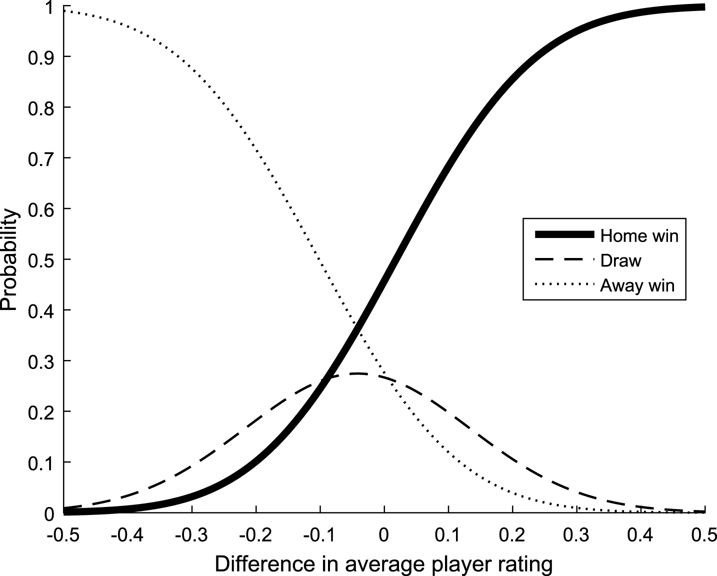
To predict match outcomes, an ordered probit regression model is used, with a single independent variable which is calculated as the difference of the average rating for the home team players and the average rating for the away team players. When simulating matches from the 2014-2015 season, the regression model is first fitted on matches from July 1 2010 to July 1 2014 using maximum likelihood estimation. The fitting of the match outcome model resulted in θ1 = -0.595, θ2 = 0.107, and γ = 5.836. All the three estimated regression coefficients are statistically different from 0, with P-values less than 10-19. For two equally good teams, the probability of a home win is 0.457, the probability for a draw is 0.267, and the probability for an away win is 0.276, reflecting the home field advantage. Figure 3 the model graphically, showing the probabilities for different match outcomes as a function of the difference in average ratings for the players in the starting lineups of two teams.
Fig.3
Match outcome probabilities from the ordered probit regression, trained using 12,267 matches between July 2011 and July 2014.
3.3Simulation of the 2014-2015 season
The 2014-2015 Premier League competition was simulated according to the specifications outlined above. Squads of players belonging to the twenty Premier League clubs were set to equal the official maximum 25 man squad of senior players, with the addition of prominent youth players. The Monte Carlo simulation returns Chelsea as the most likely champions, as shown in Table 4. The expected revenue based on their simulated final league positions is GBP229 million. Manchester City follows in second place, at GBP226.9 million. Burnley and QPR are expected to gain more modest returns from the campaign, while Aston Villa were also expected to be in the bottom three.
Table 4
Simulated league table for the 2014-2015 Premier League season, using the final team rosters, sorted by expected revenue in GBP million
| Club | Exp. rank | Actual rank | Difference in rank | Exp. points | Actual points | Difference in points | Exp. revenue |
| Chelsea | 1 | 1 | 0 | 75.4 | 87 | 11.6 | 229.0 |
| Man. City | 2 | 2 | 0 | 71.8 | 79 | 7.2 | 226.9 |
| Arsenal | 3 | 3 | 0 | 70.6 | 75 | 4.4 | 225.6 |
| Man. United | 4 | 4 | 0 | 62.4 | 70 | 7.6 | 214.2 |
| Leicester | 5 | 14 | 9 | 55.4 | 41 | –14.4 | 203.3 |
| Tottenham | 6 | 5 | –1 | 55.4 | 64 | 8.6 | 203.0 |
| Liverpool | 7 | 6 | –1 | 54.0 | 62 | 8.0 | 200.7 |
| Everton | 8 | 11 | 3 | 50.2 | 47 | –3.2 | 194.0 |
| Newcastle | 9 | 15 | 6 | 49.1 | 39 | –10.1 | 190.8 |
| West Bromwich | 10 | 13 | 3 | 49.0 | 44 | –5.0 | 191.0 |
| Stoke | 11 | 9 | –2 | 47.9 | 54 | 6.1 | 188.3 |
| Sunderland | 12 | 16 | 4 | 47.5 | 38 | –9.5 | 187.1 |
| West Ham | 13 | 12 | –1 | 47.4 | 47 | –0.4 | 186.7 |
| Southampton | 14 | 7 | –7 | 47.2 | 60 | 12.8 | 185.7 |
| Swansea | 15 | 8 | –7 | 46.5 | 56 | 9.5 | 183.4 |
| Hull | 16 | 18 | 2 | 46.0 | 35 | –11.0 | 181.3 |
| Crystal Palace | 17 | 10 | –7 | 44.5 | 48 | 3.5 | 177.8 |
| Aston Villa | 18 | 17 | –1 | 43.3 | 38 | –5.3 | 174.0 |
| QPR | 19 | 20 | 1 | 40.3 | 30 | –10.3 | 163.0 |
| Burnley | 20 | 19 | –1 | 39.7 | 33 | –6.7 | 160.5 |
There is a quite good match between the ranks predicted by the simulations and the actual ranks, with the top four teams being correctly placed by the models. The team with the biggest difference in predicted and actual rank was Leicester, predicted at fifth and ending up at fourteenth position. In the following season, Leicester performed better than most experts had foreseen, so it is tempting to suggest that their players had indeed underperformed in the 2014-2015 season.
3.4Case 1: Cesc Fàbregas
Chelsea were the actual champions of the 2014-2015 season, and Spanish midfielder Cesc Fàbregas was one of the most established players signing for the club ahead of the season. He had previously played for Chelsea’s Premier League rivals Arsenal, before spending three years in Barcelona. As Fàbregas was expected to be an important player for Chelsea, his presence in the squad should be reflected in an added value to their estimates of points and revenues. An analysis of the marginal value added by his transfer was performed by removing him from the squad of Chelsea and again simulating the competition. This scenario is equivalent to Chelsea having to compete with the same clubs, fielding the same players except Cesc Fàbregas.
The difference in simulation results is shown in Table 5. Chelsea would lose GBP2.1 million in expected revenues from their participation in the 2014-2015 Premier League by not signing Fàbregas, according to the simulation model. His presence appears to be very important in gaining an advantage over Manchester City in the competition for the title. Indeed, without Fàbregas joining Chelsea, all other clubs could expect to gain more points towards the final league table, while Chelsea would be expected to gain 3.4 points less than with the Spaniard included.
Table 5
Simulation results calculating expected points (P) and revenue (R), highlighting the hypothetical contributions of alternative choices for three key players: Lampard at Chelsea instead of Man. City, Moses at either Chelsea or QPR instead of Stoke, and Fàbregas at Barcelona instead of Chelsea
| Club | Lampard at Chelsea | Moses at Chelsea | Moses at QPR | Fabregas at Barcelona | ||||
| P | R | P | R | P | R | P | R | |
| Chelsea | 0.2 | 0.2 | 0.0 | 0.1 | –0.1 | 0.0 | -3.4 | -2.1 |
| Man. City | -1.1 | -1.0 | 0.0 | 0.0 | 0.0 | 0.0 | 0.2 | 0.3 |
| Arsenal | 0.1 | 0.1 | 0.0 | –0.1 | –0.1 | –0.1 | 0.2 | 0.3 |
| Man. United | 0.1 | 0.2 | 0.0 | 0.0 | 0.0 | 0.0 | 0.1 | 0.4 |
| Leicester | 0.0 | 0.0 | 0.0 | 0.0 | –0.1 | –0.1 | 0.2 | 0.2 |
| Tottenham | 0.1 | 0.2 | 0.0 | 0.1 | –0.1 | –0.1 | 0.2 | 0.3 |
| Liverpool | 0.0 | –0.1 | 0.0 | –0.1 | –0.2 | –0.2 | 0.1 | 0.1 |
| Everton | 0.1 | 0.2 | 0.1 | 0.1 | 0.0 | –0.1 | 0.2 | 0.1 |
| Newcastle | 0.0 | –0.1 | –0.1 | –0.1 | –0.1 | –0.4 | 0.1 | 0.0 |
| West Bromwich | 0.0 | –0.1 | 0.0 | 0.0 | –0.1 | –0.4 | 0.1 | –0.1 |
| Stoke | 0.0 | –0.1 | -0.3 | -0.8 | -0.3 | -1.0 | 0.1 | 0.0 |
| Sunderland | 0.1 | 0.2 | 0.0 | 0.1 | 0.0 | –0.4 | 0.2 | 0.1 |
| West Ham | 0.1 | 0.0 | 0.0 | –0.1 | –0.1 | –0.4 | 0.1 | 0.0 |
| Southampton | 0.0 | 0.0 | 0.0 | 0.1 | 0.0 | –0.1 | 0.2 | 0.0 |
| Swansea | 0.0 | 0.1 | 0.0 | 0.0 | –0.1 | –0.3 | 0.1 | –0.1 |
| Hull | 0.0 | –0.1 | 0.1 | 0.2 | –0.1 | –0.4 | 0.2 | 0.0 |
| Crystal Palace | 0.1 | 0.3 | 0.1 | 0.3 | 0.0 | –0.3 | 0.2 | 0.2 |
| Aston Villa | 0.1 | 0.0 | 0.0 | 0.2 | –0.1 | –0.4 | 0.1 | –0.1 |
| QPR | 0.0 | 0.0 | 0.0 | 0.0 | 1.4 | 5.2 | 0.2 | 0.1 |
| Burnley | 0.0 | 0.0 | 0.0 | 0.2 | –0.1 | –0.4 | 0.2 | 0.2 |
This analysis assumes a situation where Chelsea would refrain from obtaining a replacement instead of Fàbregas. Quite likely, if Fàbregas had not joined Chelsea, the club would have instead found a different player to take his place. By adding this alternative player to the squad instead of Fàbregas, the same methodology could be used to assess how this would influence the economic result of Chelsea, and hence also to evaluate which option to prefer, taking into account the costs to obtain Fàbregas and the alternative player.
3.5Case 2: Frank Lampard
Chelsea parted company with a highly rated midfielder before the season. Frank Lampard left to join New York City on a free transfer. The American team is an affiliate club of Manchester City, and Lampard proceeded to join the latter on a loan deal for the entire 2014-2015 Premier League season. This provoked some debate as to whether Chelsea should have sought to keep the midfielder, rather than lose him to a rival. The league simulation in Table 4 was performed with Lampard as part of Manchester City’s squad. By removing him from their disposal and moving him back to Chelsea instead, we can estimate the value he would add to City’s campaign.
The loss of Lampard is estimated to imply a loss of GBP1.0 million for Manchester City, while Chelsea would gain only GBP0.2 million by keeping him. Lampard’s presence at City helps build an advantage over rivals Arsenal, who would otherwise be expected to finish on the same number of points.
3.6Case 3: Victor Moses
The simulation model as set up in this work is perhaps most suitable for evaluating loan agreements, analysing the potential value added by a player moving temporarily to a rival club. Victor Moses was recruited by Chelsea in 2012. He featured frequently for their first team in the 2012-2013 season, before spending all of the following season on loan at Liverpool. In the summer of 2014, Chelsea appeared to be faced with three options: keeping Moses at the club, selling him, or loaning him to another club. They chose to loan him to Stoke City for the whole season.
As our original simulation included Moses as part of Stoke City’s squad, we can assess his value to both them and Chelsea by moving him back to his parent club. Doing so indicates a marginal value estimate of GBP0.8 million to Stoke City and only GBP0.1 million to Chelsea. The value Moses adds to Stoke City appears to be significant, but not dramatic. For the sake of inquiry, we also examine the potential of Moses being more valuable to a different club. Queens Park Rangers could possibly offer Moses the opportunity of regular playing time in the Premier League without moving away from London. They were also expected to struggle against relegation towards the bottom of the table. By moving Victor Moses from Stoke City to QPR, we estimate his marginal value to QPR for the season to be GBP5.2 million. QPR are still expected to finish second last, even with Moses, but they finish 17th or higher in a much larger proportion of the simulations than before.
4Concluding remarks
This paper presented a framework for evaluating the contribution of soccer players to the financial success of their club. The framework consists of three parts: a method to evaluate the quality of each player, a method to translate the quality of players in the starting lineups to probabilities for match outcomes, and a method to simulate the relevant soccer competitions with the help of calculated match outcome probabilities. To illustrate the framework, a simple top-down player rating based on the plus-minus rating principle was developed. An ordered probit regression model was used to determine probabilities for match outcomes, and Monte Carlo simulation was used to simulate a league competition.
Case studies illustrated the use of the framework to value player transfers in the English Premier League during the 2014-2015 season. Running simulations based on alternative squads for the clubs involved, the value of specific player transfers can be estimated. For example, it was found that if Chelsea player Victor Moses had been loaned to QPR instead of Stoke, QPR would increase their expected number of points by 1.4 and their expected revenue by GBP5.2 million, as their risk of being relegated would be reduced.
The framework can be used in practice after only a few modifications. First, it will be beneficial to simulate more competitions, such as the European cups, the national cups, and lower divisions. In this way, better estimates of the true revenue potential can be gained, as well as a better understanding of the variability of the revenues. Second, it will be beneficial to simulate more than one season, so that the value of relegation and promotion can be accurately calculated, and such that the effect of players with ending contracts can be gauged. Third, when assessing player transfers, the framework currently identifies the marginal revenue of players, while the fixed revenues are allocated to the existing players. However, all players involved in matches should receive some credit for their share of the revenues that are secured simply by having a team available.
This in turn implies that the valuations of players using the framework is currently too low, as only the marginal value of a player relative to an existing squad is assessed. The fixed income from having enough players to participate with a team, should be distributed among all the players. In addition, each player may have a marquee value effect (Gennaro, 2007) whereby star players draw greater attention from supporters, sponsors and media. This added value also manifests itself in increased sales of merchandise, sponsorships and endorsement packages, as well as ordinary and corporate ticket packages.
Using the framework implies that important directions for future research can be described. First, the development of better player ratings becomes more important, as more accurate ratings will allow more accurately to calculate the true value of a given player. Second, improved match predictions become important for the clubs. While this work only included the player ratings to predict match outcomes, other factors such as travel distance and match importance (Goddard, 2005), as well as playing surfaces (Hvattum, 2015), can be included. Third, to take into account player fatigue, long term injuries, or the relative importance of matches as a consequence of the league standings, discrete event simulation may be more appropriate than a simple Monte Carlo simulation of the competitions involved. Nevertheless, the framework in its current form provides a useful basis for evaluating alternative player transfers, for example when considering whether to sign a new defender or a new forward.
Acknowledgments
The authors thank an anonymous reviewer and the Editor-in-chief for insightful comments that helped to improve the manuscript.
References
1 | Constantinou A.C. and Fenton N.E., (2013) , Determining the level of ability of football teams by dynamic ratings based on the relative discrepancies in scores between adversaries, Journal of Quantitative Analysis in Sports 9: , 37–50. |
2 | Constantinou A.C , Fenton N.E. and Neil M., (2012) , pi-football: A Bayesian network model for forecasting association football match outcomes, Knowledge-Based Systems 36: , 322–339. |
3 | Dixon M.J. and Coles S.G., (1997) , Modelling association football scores and inefficiencies in the football betting market, Journal of the Royal Statistical Society: Series C (Applied Statistics) 46: , 265–280. |
4 | Dobson S. and Goddard J., (2001) , The Economics of Football. Cambridge. |
5 | Frick B. , (2007) , The football players’ labor market, Scottish Journal of Political Economy 54: , 422–446. |
6 | Gennaro V. , (2007) , Diamond Dollars: The Economics of Winning in Baseball, Diamond Analytics, Purchase, New York. |
7 | Gerrard B. , (2014) , Achieving transactional efficiency in professional team sports: The theory and practice of player valuation. In Goddard J. and Sloane P., editors, Handbook on the Economics of Professional Football, pages 189–202. Edward Elgar Publishing, Cheltenham, U.K. |
8 | Goddard J. , (2005) , Regression models for forecasting goals and match results in association football, International Journal of Forecasting 21: , 331–340. |
9 | Harris N., Where the money went: Liverpool top Premier League prize cash in 2013-14. http://www.sportingintelligence.com/2014/05/14/where-the-money-went-liverpool-top-premier-leagueprize-cash-in-2013-14-140501/, May 2014. Last accessed 9 June 2015. |
10 | Herm S , Callsen-Bracker H.-M. and Kreis H., (2014) , When the crowd evaluates soccer players’ market values: Accuracy and evaluation attributes of an online community, Sport Management Review 17: , 484–492. |
11 | Hvattum L.M. , (2013) , Analyzing information efficiency in the betting market for association football league winners, The Journal of Prediction Markets 7: , 55–70. |
12 | Hvattum L.M. , (2015) , Playing on artificial turf may be an advantage for Norwegian soccer teams, Journal of Quantitative Analysis in Sports 11: , 183–192. |
13 | Hvattum L.M. and Arntzen H., (2010) , Using ELO ratings for match result prediction in association football, International Journal of Forecasting 26: , 460–470. |
14 | Lasek J , Szlávik Z. and Bhulai S., (2013) , The predictive power of ranking systems in association football, Inter-national Journal of Applied Pattern Recognition 1: , 27–46. |
15 | Leitner C , Zeileis A. and Hornik K., (2009) , Forecasting sports tournaments by ratings of (prob)abilities: A comparison for the EURO 2008, International Journal of Forecasting 26: , 471–481. |
16 | Macdonald B. , (2011) , An improved adjusted plus-minus statistic for NHL players, Proceedings of the MIT Sloan Sports Analytics Conference. |
17 | Macdonald B. , (2012) , Adjusted plus-minus for NHL players using ridge regression with goals, shots, Fenwick, and Corsi, Journal of Quantitative Analysis in Sports 8: . |
18 | McHale I.G , Scarf P.A. and Folker D.E., (2012) , On the development of a soccer player performance rating system for the English Premier League, Interfaces 42: , 339–351. |
19 | Min B , Kim J , Choe C , Eom H. and McKay R.I., (2008) , A compound framework for sports results prediction: A football case study, Knowledge-Based Systems 21: , 551–562. |
20 | Ruijg J. and van Ophem H., (2015) , Determinants of football transfers, Applied Economics Letters 22: , 12–19. |
21 | Sæbø O.D. and Hvattum L.M. , (2015) , Evaluating the efficiency of the association football transfer market using regression based player ratings. In NIK: Norsk Informatikkonferanse, Bibsys Open Journal Systems 12 pages. |
22 | Scully G.W. , (1974) , Pay and performance in Major League Baseball, American Economic Review 64: , 915–930. |
23 | Sloane P.J. , (1971) , The economics of professional football, Scottish Journal of Political Economy 18: , 121–146. |
24 | Sloane P.J. , (2015) , The economics of professional football revisited, Scottish Journal of Political Economy 62: , 1–7. |
25 | Szymanski S. and Zimbalist A., (2005) , National pastime; how americans play baseball and the rest of the world plays soccer, Washington DC: Brookings Institution Press. |
26 | Tunaru R. and Viney H., (2010) , Valuations of soccer players from statistical performance data, Journal of Quan-titative Analysis in Sports 6: ((2)), 10. |
27 | Tunaru R , Clark E. and Viney H., (2005) , An option pricing framework for valuation of football players, Review of Financial Economics 14: , 281–295. |
28 | Vrooman J. , (2007) , Theory of the beautiful game: The unification of european football, Scottish Journal of Political Economy 54: , 314–354. |
29 | Winston W.L. , (2009) , Mathletics. Princeton University Press. |
30 | Witten I.H. and Frank E., (2005) , Data mining: Practical machine learning tools and techniques, Elsevier, San Francisco, CA. |


