
Winner prediction in an ongoing one day international cricket match
Abstract
Cricket is a team sport with an intricate set of rules, where players specialize in multiple skills such as batting, bowling, and fielding. Playing conditions and home advantage also impact the game. Thus, it is quite challenging to build an accurate quantitative model for the game. In this paper, we provide a data driven approach to predict the winner of a cricket match. We divide the ongoing match into various states and provide a prediction for each state using supervised machine learning models. We employ dynamic features that account for the current match situation, together with the static features like team strength, winner of the toss, and the home advantage. We also use SHAP scores—an explainable AI technique—to interpret the proposed prediction model. We use ball-by-ball data from 1359 men’s one day international cricket matches played between January 2004 to January 2022 to present our results. We achieved the best in-play prediction accuracy of about 85% . SHAP scores reveal that during initial phases of the match, the model treats static features like team strength more important than others, in making the predictions. But as the match progresses, dynamic features capturing the current match situation become exceedingly important. Our work may be useful in preparing tools for in-play winner prediction for live cricket matches that can be used in websites and mobile applications covering the sport, in providing analytics during live television commentary, and in legal betting platforms.
1Introduction
One hundred and four member countries constitute the International Cricket Council (2023), the governing body for cricket. This includes 12 full members and 92 associate members. Smith (2023) estimates that 2.5 billion people follow cricket around the world. Together they amassed 13.7 billion viewing hours during the most recent quadrennial one day international (ODI) world cup that took place in 2019. These statistics show the popularity of cricket among the world population, and the amount of economic impact it can generate if harnessed optimally.
Cricket has a large and complex set of rules. It is a team sport in which players specialize in multiple skills—batting, bowling, and fielding. Thus, creating an accurate quantitative model of the game is a difficult task. In this paper we provide a supervised machine learning framework to predict the winner of an ODI match. We make in-play predictions for every over of the match, keeping the current match status in mind. We have also accounted for factors such as team strength, home conditions, etc. in our framework. We train and test our machine learning model on a dataset of 1359 men’s ODI matches played between January 2004 to January 2022. We were able to achieve the best in-play prediction accuracy of about 85% . We have used explainable AI techniques to provide insights about how the prediction model works. Our work may be useful in providing analytics in sports websites that provide ball-by-ball updates of a cricket match, or during live television commentary. Other possible applications include legal betting platforms which have a huge market. For example, the report of IFSG-AC Neilson estimates that 67 percent of Indian cricket match viewers are aware of fantasy sports mobile applications—a form of legal betting—and these applications have a loyal user base (Media Infoline, 2018).
1.1Related work and our contributions
In this section, we discuss past literature that uses statistical and machine learning tools in cricket and other sports. Researchers have used different techniques (e.g., supervised learning, reinforcement learning, etc.) to achieve different objectives (e.g., match outcome prediction, player evaluation, etc.). Muazu Musa et al. (2019) have used a supervised learning approach to identify high caliber archers from a pool of 50 youth archers. In a separate work, Liu and Schulte (2018) have used a reinforcement learning based method to evaluate players’ performances in ice hockey.
The winner prediction problem addressed in this paper has been undertaken earlier for other sports. Owramipur et al. (2013) and Berrar et al. (2019) have predicted the winner of a football match using Bayesian networks, and classifications techniques (like k-NN and XGBoost). The key observation made was that the domain knowledge of the sport improves the accuracy of prediction. Similar studies were done for National Basketball Association (NBA) league matches (Chen et al., 2020) and horse racing (Davoodi and Khanteymoori, 2010) using neural networks.
We now discuss the literature on cricket that uses various statistical techniques on the past data to analyze players’/teams’ performances. Mukherjee (2014) used a network science-based page-rank algorithm to rank cricket players in test and ODI matches. Similar techniques were used by Daud et al. (2015) to rank teams instead of individual players, and Roy et al. (2017) to rank both players and teams. A related problem is to determine optimal team line-ups which was addressed by Kamble et al. (2011); Perera et al. (2016); and Passi and Pandey (2018) using standard decision-making techniques, match simulation, and machine learning tools. We also consider players’ performance in our work to quantify relative strengths of the competing teams. However, this is just one of the factors that play a role in the overall prediction problem that we address.
Machine learning techniques have been extensively used in cricket as well. Kaluarachchi and Aparna (2010) predicted the winner of an ODI match based on features such as home advantage, day/night effect, outcome of the toss, and the team’s decision to bat/bowl first. The authors made a static decision that did not change as the match progressed. Similarly, Jhanwar and Pudi (2016) used home advantage, toss, and the team strengths to make a static prediction for the winner at the beginning of an ODI match. Rahman et al. (2018) improved the framework by providing a prediction not just at the beginning of the match, but also after completion of the first innings, and at fall of wickets. However, the study was conducted for a single country only.
In contrast to the above literature, our work addresses the in-play prediction problem—which is dynamic in nature—such as the ones discussed by Sankaranarayanan et al. (2014), Bailey and Clarke (2006), and Viswanadha et al. (2017). The problem addressed by Sankaranarayanan et al. (2014) and Bailey and Clarke (2006) are slightly different from our work, in that they predict the runs scored by the competing teams (and hence, the winners, indirectly). Unlike our work, these papers did not employ classification techniques; rather, they used regression models. Given the current state of the match and the historical data, our work directly trains classifiers to predict the winner. Viswanadha et al. (2017) also used a framework similar to the one used in our work; however, that study was conducted for a local T20 league and the features set was also limited. Also, the prediction was done for only the second innings of the match. In contrast, we predict the winner in both the innings.
In addition, we also explain model predictions using SHAP scores (Lundberg & Lee, 2017) and identify the features that contribute the most in making the predictions at various stages of the match. Although explainable AI techniques have been used to interpret model outputs in sports before—for example, Wang et al. (2022) have used the LIME framework for basketball—to the best of our knowledge, such techniques have not been used in the context of cricket in the past literature. Hence, the previous literature on limited overs cricket, even the ones closest to our work (Viswanadha et al., 2017), cannot provide such insights.
Rest of this paper is organized as follows. In Section 2 we pose the winner prediction problem as a machine learning classification problem. To this end, the methodology to quantify the players’ and teams’ performances is present in Section 3. The dataset used in this work is discussed in Section 4, and further analyzed in Section 5. Section 6 discusses the experimental results. The prediction models are explained using SHAP scores in Section 7, and finally the paper concludes in Section 8.
2Preliminaries and problem statement
In this section, we first provide a brief overview of an ODI match and then discuss the mathematical notations used to describe the game. Then, we formulate the winner prediction classification problem and explain the features used for classification. A cricket match is played in three formats –a test match, an ODI match, and a twenty-twenty (T20) match. Similar to the other formats, an ODI match is contested between two teams of 11 players each. A specific match can be broken down into a number of different parts for analysis. The match is divided into 2 innings of (a maximum of) 50 overs each, with each over consisting of 6 (valid) deliveries. Thus, an innings consists of a maximum of 50×6 = 300 deliveries. An innings is the length of time a team bats or bowls. In a specific game, each team gets a chance to bat and bowl in one of the two innings.
The game begins with a coin toss. The team winning the toss exercises the option of either batting or bowling/fielding in the first innings. This choice provides a slightly advantageous position to this team as it can exploit the match conditions in a better manner1. The team batting first sets a specific target for the other team by scoring a specified number of runs, and the team batting second chases that target. If all the deliveries have been bowled, or the chasing team loses all 10 wickets, the target would not be attained; leading to a loss for the chasing team.
Now we discuss the mathematical notations used in the classification problem and the features used in this paper. The first and the second innings of a given ODI match M is represented as I1 and I2 respectively. Each innings of M is divided into 50 distinct states Sk, where 0≤k≤49. We define the term state as the progress of the innings at the end of each over. Thus, Sk represents the state of the innings before the (k + 1)th over, or after the kth over has been bowled. We predict the winner at each of these states leading to 50 predictions for each innings.
The prediction at S0 in I1 is the prediction even before the first ball has been bowled in the match. The state S0 in I2 (which is equivalent to the state S50 of I1, had S50 been defined) represents the match progress at the end of I1 or before the start of the 1st over in I2. Similarly, S49 in I2 represents the end of the 49th over. Note that, S50, the end of the 50th over in I2 is not taken into consideration because the match outcome is already known by that point. We call the team batting first as Team A, and the team batting second as Team B. The goal is to dynamically forecast whether Team B wins or loses in the state Sk, where 0≤k≤49, for I1 and I2 in a given match M. Note that the forecast adapts to the current progress of the match. This transforms into a machine learning classification problem which requires a certain set of features. In this paper, we consider six features to train the machine learning classifiers which are defined as follows:
1. Balls Remaining: This feature represents the number of deliveries that remain at each state of the innings. There are a total of 50 overs of 6 deliveries each in an innings. So, balls remaining at each state Sk is Bk = (300 –k×6) where 0≤k≤49.
2. Lead of Team A: In the first innings I1, the lead of Team A at any state Sk is the runs scored by Team A by that state. The same is defined in I2 as follows. Let the total runs scored by Team A at the end of I1 be RA, and the runs scored by Team B at the state Sk be rBk. Then, the lead of Team A for that state is RA –rBk.
3. Wickets Remaining: The wickets remaining is computed for the batting team in each state of the innings. The total wickets remaining at the state Sk is defined as 10 –Wk, where Wk = the number of wickets lost by the batting team till state Sk.
4. Relative Team Strength: This feature quantifies the strengths of the competing teams based on the historical data of the players of the teams. Each player is assigned a value according to his batting and bowling performances, then the team strength is computed based on the values of the team members. We discuss this feature in detail in Section 3.
5. Home Country: This feature is assigned a value of 1 if the match is being played in the home country of Team B, 0 if the match is being played in the home country of Team A, and 0.5 if the match is being played at a neutral venue.
6. Toss: This feature is assigned a value of 1 if Team B wins the toss, otherwise it is 0.
Apart from these features, each data point has a class label. The class label is set to 1 when Team B wins the match, otherwise it is set to 0. The selection of features in this study is partially inspired by the work by Morley and Thomas (2005) which concluded that the toss, team quality (relative team strength), and the home advantage are important features in determining the outcome of a match. These features are static throughout the match and bias the outcome towards a certain team, hence, useful in prediction. Also, for the in-play prediction during the progress of the match it is natural to consider features that are dynamic in nature. These features—resources remaining (balls and wickets) and current run difference between the teams—capture the current status of the match, and were also used by Viswanadha et al. (2017). However, as stated earlier, unlike our work which is conducted on international matches, both of these past studies were conducted on local leagues.
3Methodology
In this section, we present a method to assign a value or score to a batsman and a bowler based on their past performances. These values are used to compute the feature “relative team strength” which is explained later in the section.
3.1Player’s valuation
We discuss methods to quantify a batsman’s and a bowler’s performance. The parameters used here are standard ways of evaluating a player’s performance in cricket.
3.1.1Batsman’s valuation
A batsman’s skill is a combination of his ability to stay on the pitch and to score runs without wasting the deliveries faced. The batting score of a player is calculated on the basis of the two parameters that capture these abilities—the batting average and the batting strike rate. They are defined as follows:
Batting Average (BaAv): It is the average number of runs scored by a batsman before getting out. It is calculated by dividing the total runs scored by the batsman (RSc) by the number of times he has been out (Out) in his career.
We have calculated BaAv based on ball-by-ball data of all the matches in the training dataset. For batsmen who got dismissed fewer than 4 times in the whole training dataset (which consists of 760 matches and is discussed later), BaAv is capped to 25. This is because of the lack of data to justify an extraordinary standing as a consistent run scorer.
Batting Strike Rate (BaSR): For a batsman, it is the average runs scored for every 100 balls he faced:
Here, RSc is the number of runs scored by the player in the training dataset, and BF is the number of balls faced by the player in the training dataset. For batsmen who have faced 50 or fewer balls in the entire training dataset, BaSR is capped to 80.
Since these two parameters characterize a batsman, the batsman’s valuation (BaSc) is calculated as the product of both of them:
3.1.2Bowler’s valuation
The bowling score can be evaluated on the basis of two parameters—the bowling economy and the bowling strike rate. A better bowler is expected to have a lower economy and a lower strike rate. These parameters are defined as follows:
Bowling Economy (BoEc): Also known as economy rate, it is the average number of runs a bowler concedes per over bowled:
Bowling Strike Rate (BoSR): It is defined as the average number of balls bowled per wicket taken by a bowler. It accounts for the high wicket-taking ability for a bowler:
Note that these two quantities are inversely proportional to the bowler’s quality. Hence, the bowler’s valuation (BoSc) is the reciprocated product of these two parameters:
If a player did not bat or bowl in the entire training dataset, we set the corresponding valuations, BaSc or BoSc, as 0. An extremely good parameter value for bowling and/or batting statistics could be a result of players doing well in a very short career of a few games. Therefore, the capping was carried out. These capping criteria were subjectively decided based on the overall pattern of good and bad batting and bowling statistics for the players that are known to be good in their skills. In any case, an extraordinary player is not likely to have a very short career (which led him to face only 50 or fewer balls as a batsman, or bowl less than 6 overs as a bowler in the entire training dataset).
3.2Team rating
The method used to determine the relative team strength is similar to that used by Viswanadha et al. (2017) and is present in Table 1. The quality of Team B (the team batting second) with respect to Team A (the team batting first) is referred to as the relative team strength in the present context. Therefore, the inputs to the algorithm presented in Table 1 are the set of all matches in the training dataset M, and the valuations of all the batsmen and bowlers who participated in those matches.
Table 1
Algorithm to calculate the relative team strength
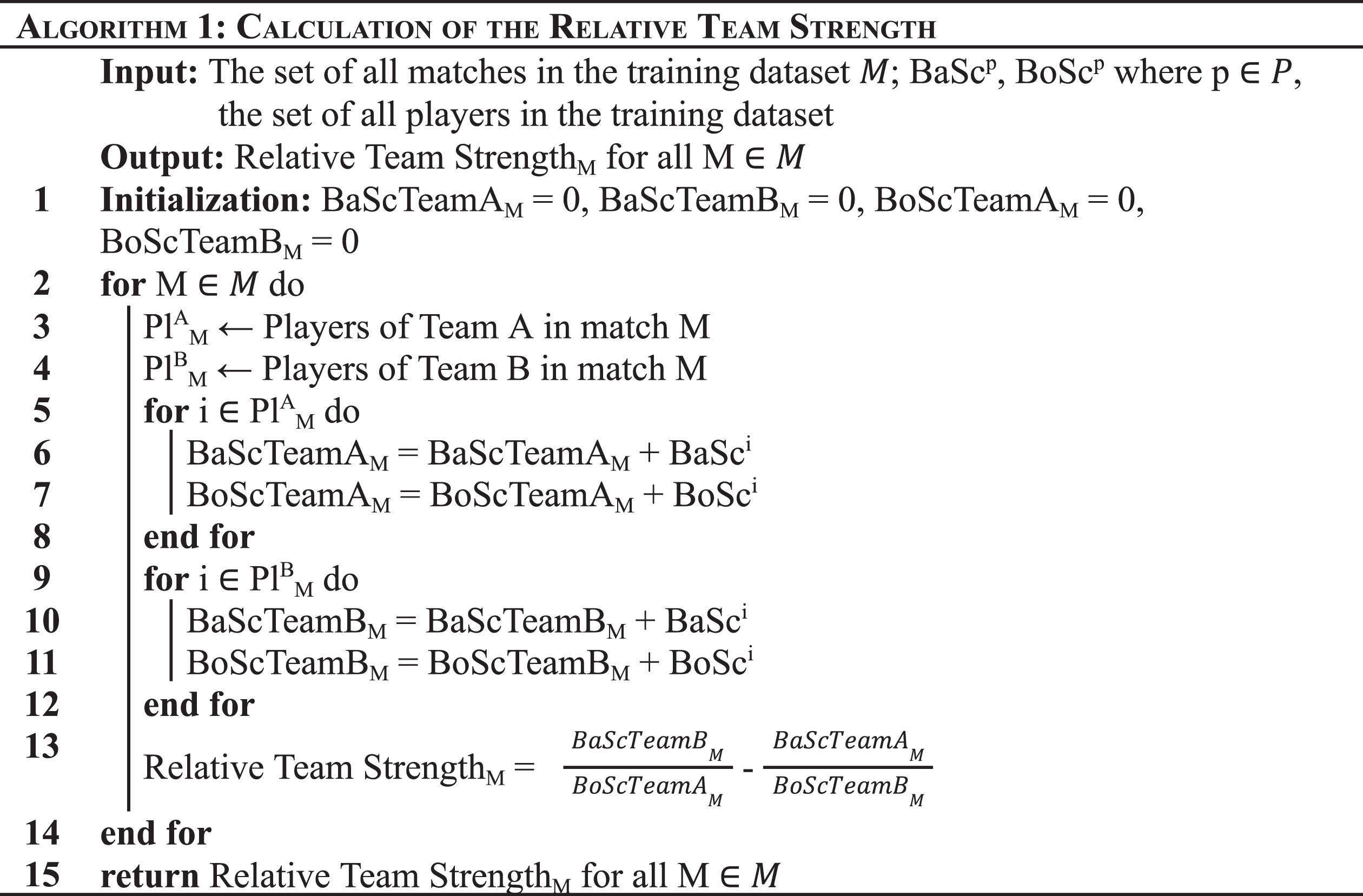 |
This algorithm iterates through the matches after doing the appropriate initializations. The players who participated in the game are fetched as each game is iterated. Each team’s batting and bowling scores are calculated by adding the individual batsman’s and bowler’s valuations. In other words, we take the contribution of all 11 players of the respective teams.
4Dataset: Mining and preparation
We transform the publicly accessible raw data into the necessary structured format for application to the machine learning algorithms. The curated dataset is applied to conventional classification techniques that learn from the features mentioned in Section 2 in order to forecast the data point’s label.
4.1Data mining
The raw data used in this paper is available in the Cricsheet website maintained by Rushe (2023). The dataset consists of 2240 distinct one day international matches played between January 2004 and January 2022. Ball-by-ball data of each ODI match is present in the ‘.json’ file type format. We convert this into Python usable dataframes. We consider only Men’s ODIs—excluding the non-international and the women’s ODIs. This is because the scoring pattern and match dynamics vary significantly over these parameters. Also, only matches played between 10 full members of the International Cricket Council are considered. These countries include India, Pakistan, Bangladesh, Sri Lanka, Zimbabwe, South Africa, Australia, New Zealand, England, and West Indies. This is to avoid teams with very few matches in the whole dataset.
The curtailed matches—those interrupted by rain or bad weather conditions, and decided by Duckworth and Lewis (1998) method in either innings—are also excluded. Other incomplete or tied matches were also excluded from the dataset. This resulted in a total of 1359 valid complete men’s ODI matches that constitute our whole dataset.
4.2Data preparation
The 1359 matches obtained above are split into three groups for training, validating (hyperparameter tuning), and testing the machine learning models. We keep about 25% of the matches for testing, leading to a testing dataset of size 340 matches (randomly chosen from the pool of 1359 matches). Of the remaining 75% of the 1359 matches (1019 matches), 760 matches are chosen for the training dataset and 259 matches are chosen for the validation dataset. This is again a random split of 75% –25% of the 1019 matches.
The nature of the data is different in the first and the second innings. For example, balls and wickets remaining is always calculated for the team batting in the concerned innings of the particular match, which changes abruptly as the innings changes. Thus, we have handled the predictions for the first and the second innings separately. The six features discussed in Section 2 are determined for each state of the first and the second innings. A single classifier is trained on the data of all the states of the first innings. Similarly, another classifier is trained on all the data of the second innings.
Three features are constant throughout the ODI match—relative team strength, home country, and toss—hence, they are computed only once for a particular match. Rest of the three features—balls remaining, wickets remaining, and lead of Team A—changes with the match state, and are computed once for each state of the first and the second innings. To compute the relative team strength, we need players’ valuations for the playing eleven of the participating teams. The players’ valuations—for the 760, 259, and 340 matches in the training, validation, and testing datasets respectively—are computed using the data from the 760 matches in the training dataset only. This was done to avoid using the data from the testing dataset during training and hyperparameter tuning of the models. However, this leads to an ambiguity when a new (unknown) player is encountered in the validation and the testing dataset, which is discussed below.
The unknown player situation: To obtain the valuation of the unknown player, we determine the playing role (batsman/bowler/all-rounder) of the new player manually with the help of ESPN Cricinfo (2023) website. We compute the batting and the bowling valuations based on the statistics set in Table 2. The statistics are set in accordance to the performance of the average player (of the given playing role) in the players’ pool of the training dataset.
Table 2
Statistics for the unknown player in the validation and test datasets
| Playing Role | Players’ Statistics |
| Batsman | Batting Strike Rate = 80 |
| Batting Average = 25 | |
| Bowler | Batting Strike Rate = 60 |
| Batting Average = 8 | |
| Bowling Economy = 5 | |
| Bowling Strike Rate = 45 | |
| All Rounder | Batting Strike Rate = 80 |
| Batting Average = 25 | |
| Bowling Economy = 5 | |
| Bowling Strike Rate = 45 |
We do not have the same number of training points for all the states of each innings. When the team batting first (Team A) gets all out before 50 overs, the data points beyond the state where the innings finished, do not exist for the first innings. Similarly, if Team B chases the score successfully, or gets all out before 50 overs of the second innings; the data points do not exist beyond this state. Hence, all states in the respective innings have potentially different numbers of training/validation/testing data points.
5Data analysis
In this section, we familiarize ourselves with the (training) data that is available to us, and analyze the curated (training) dataset. We will demonstrate that the features considered in Section 2 vary for class labels 0 (Team B losing) and 1 (Team B winning), and hence useful for classification purposes.
The training dataset has 381 matches in which Team B lost, and 379 matches in which Team B won. These matches led to 18865 and 17757 training data points for class labels 0 and 1 respectively in the first innings; and, 16915 and 15701 training data points for class labels 0 and 1 respectively in the second innings. These numbers show that we have an almost balanced dataset with respect to the class labels.
We plot the features that stay constant for all the states in the first and the second innings in Figs. 1, 2 and 3. We use box plot to represent the ‘relative team strength’, and histograms to represent ‘home country’ and ‘toss’ features. Recall that the ‘relative team strength’ is computed for Team B, with respect to Team A. For this feature, the ability to differentiate between labels 0 and 1 (Team B winning), which appears on X-axis, is demonstrated in Fig. 1. As expected, for label 1, the distribution of the feature shifts upwards as compared to that for label 0.
Fig. 1
Relative Team Strength vs. Team B won.
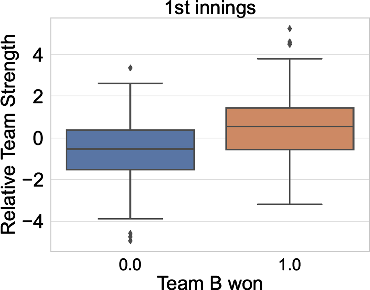
Fig. 2
Match count w.r.t. Home country advantage.
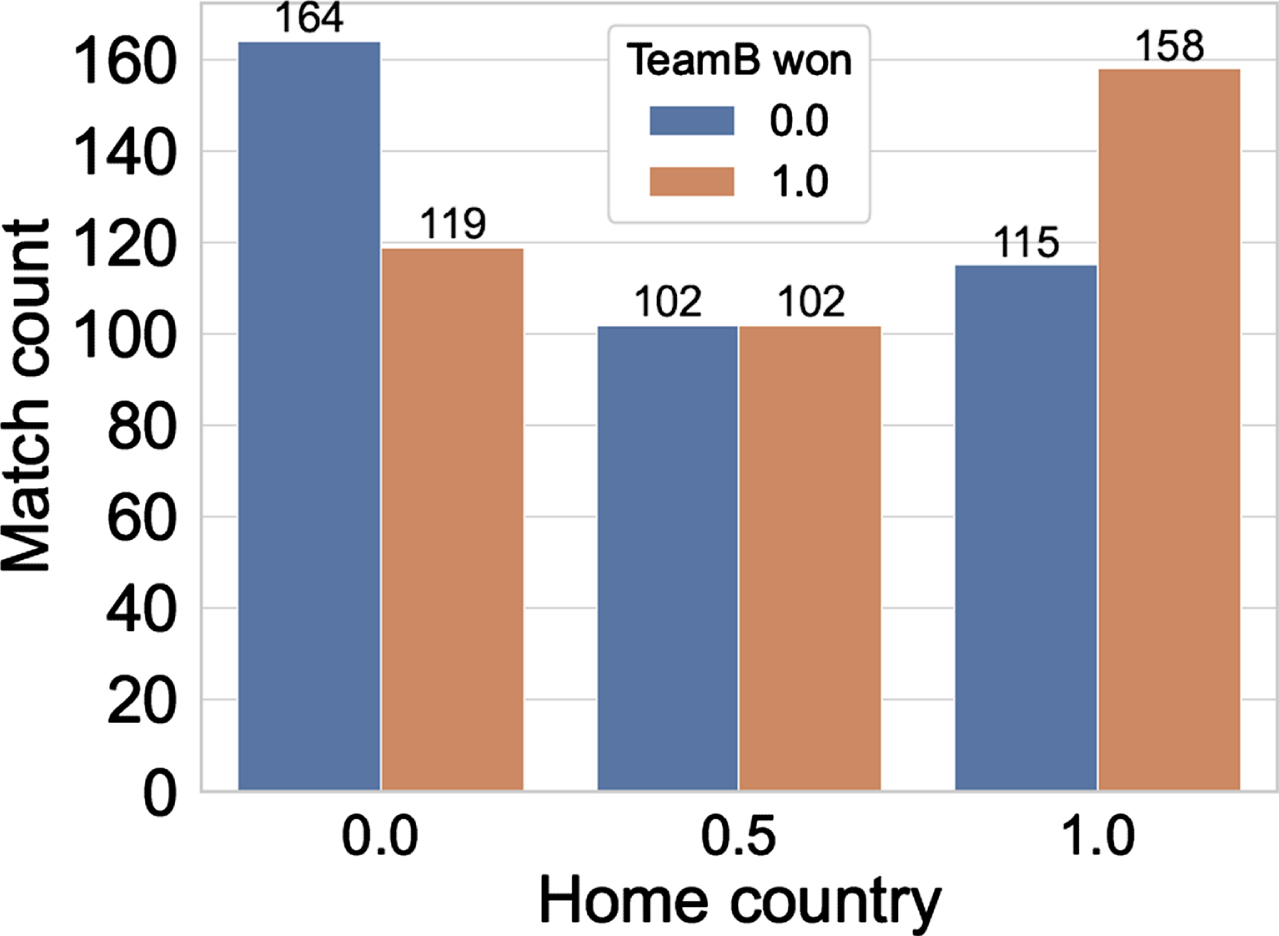
Fig. 3
Match count w.r.t. Toss. Feature value is 1 if Team B wins the toss.
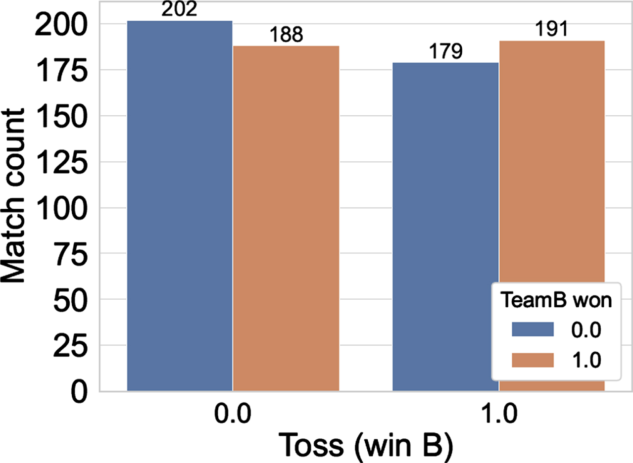
Figure 2 plots the count of the matches for the cases when the matches are being played in the home country of Team B (represented by feature value of 1.0 in the X-axis), the neutral venue (represented by feature value of 0.5), and the home country of Team A (represented by feature value of 0). In our data, teams playing in their home countries are more likely to win the matches (home teams win 57.91% of the matches, excluding matches played in the neutral venues), also the win likelihood is almost equal in the neutral venues. A similar trend was observed in the study by Morley and Thomas (2005); however, that study was conducted for the English county matches. Figure 3 shows the effect of toss on the matches, 51.71% of the matches were won by the team winning the toss. Again, this agrees with the past study of Morley and Thomas (2005).
Fig. 4
Balls Remaining vs Team B won (for 1st innings).
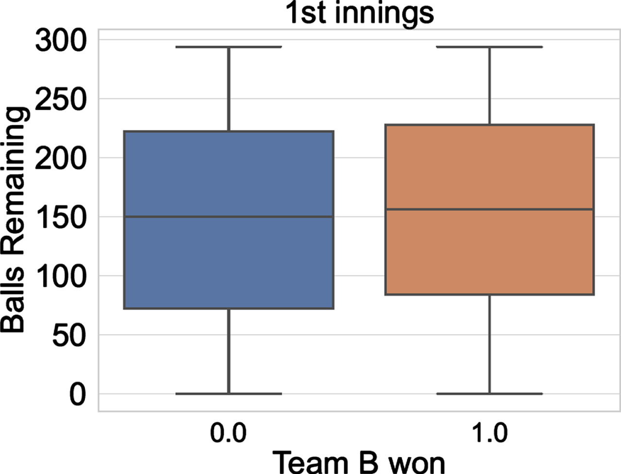
Now we discuss the dynamic features that change with the innings and states—‘balls remaining’, ‘lead of Team A’ and ‘wickets remaining’. The predictive strength of the feature ‘lead of Team A’ is demonstrated by the difference in the distribution of the data with respect to the class labels. This is observed in Figs. 5 and 8.
Fig. 5
Lead of Team A vs Team B won (for 1st innings).
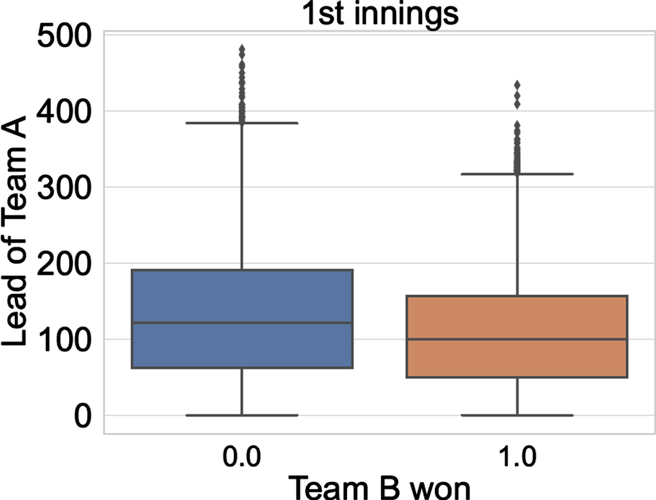
Fig. 6
Wickets Remaining for the batting team vs Team B won (for 1st innings).
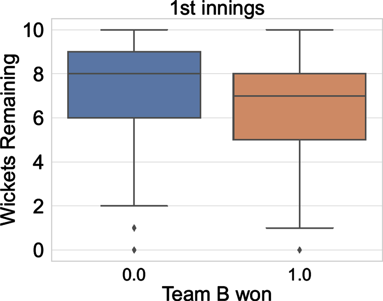
Fig. 7
Balls Remaining vs Team B won (for 2nd innings).
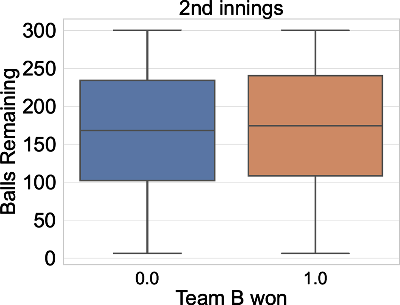
Fig. 8
Lead of Team A vs Team B won (for 2nd innings).
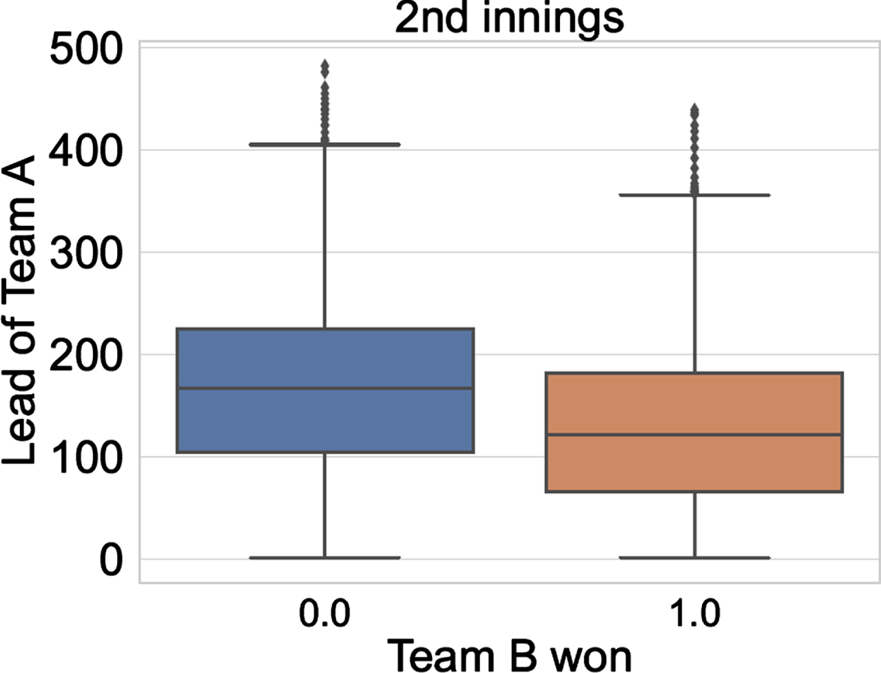
We can notice that the lead of Team A is higher when Team B loses (label 0 on X-axis in both the figures); and the lead of Team A is lower when Team B wins (label 1 on X-axis in both the figures). In both the figures, the lead of Team A is higher when Team A wins the match.
Similarly, the predictive strength of the feature ‘wickets remaining’ (of the batting team) is shown in Figs. 6 and 9. Figure 6 plots the wickets remaining for the batting team A in the first innings. We observe from the figure that when Team B wins (label 1 on the X-axis), the value of this feature is lower compared to the case when Team B loses (label 0 on the X-axis). Figure 9 plots the wickets remaining for the batting team B in the second innings. When Team B wins (label 1 on the X-axis), the value of this feature is higher compared to the case when Team B loses (label 0 on the X-axis). In both the figures, wickets remaining of the batting team is higher when the batting team wins, demonstrating the predictive strength of this feature. Figures 10 and 11 shows the heat map of the features for both the innings for the training set. The correlation between the features is as expected. Here, we highlight a few significant points: (i) In both the innings, ‘lead of Team A’ is negatively correlated with ‘relative team strength’ and ‘home country’ advantage (both of which are computed for Team B with respect to Team A). In other words, as one would expect, when Team B is stronger, or when the match is being played in the home of Team B; the lead of team A is lower. (ii) In the first innings ‘wickets remaining’ (for Team A) is negatively correlated with ‘relative team strength’ (of B over A); similarly, in the second innings ‘wickets remaining’ (which is computed for Team B) is positively correlated with ‘relative team strength’ (of B over A). Again, as expected, the feature ‘wickets remaining’ tilts in favor of the stronger team.
Fig. 9
Wickets Remaining for the batting team vs Team B won (for 2nd innings).
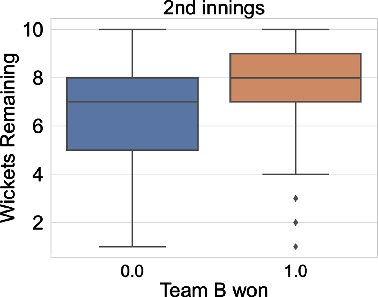
Fig. 10
Heatmap for the features (for 1st innings).
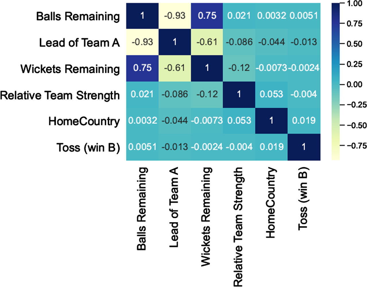
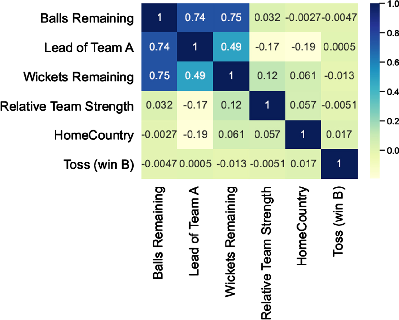
The three dynamic features—‘balls remaining’, ‘lead of Team A’ and ‘wickets remaining’—are intertwined with each other, and should only be considered together. For example, consider the following two scenarios in the second innings: In both first and the second scenarios, the lead of Team A is 100, and wickets remaining for the batting team B is 7. In the first scenario, the number of balls remaining is 60, whereas, in the second scenario, it is 180. Team B is more likely to win in the second scenario than the first. Thus, the predictive strength of these features become significant only when considered together. However, these three dynamic features are interrelated. As the innings progresses, balls remaining decreases and so do the wickets remaining. Also, with progress of the innings, the lead of Team A increases in the first innings, and decreases in the second innings. This inter-relation between the three dynamic features is also evident from the high degree of correlation between them as can be seen from the heat maps for the features for the first and the second innings shown in Figs. 10 and 11 respectively.
Given the correlated nature of these three dynamic features, it is not clear if the classification models would assign same importance to all the features or would treat some of the features (and if so, which ones) more important than others. The model interpretability study undertaken by us (details are in Section 7) reveals that the ‘balls remaining’ feature is treated as less important than the other two dynamic features. We would like to emphasize that, in the context of limited overs cricket, previous literature has not used explainable AI concepts to interpret the classification models; hence, cannot provide such insights about the model.
Fig. 11
Heatmap for the features (for 2nd innings).
6Experiments and results
The computed features for the first and second innings are used to train separate classifiers for the two innings. We make a prediction of the winner of an ongoing ODI match for each of the 50 states in both the innings using the following standard machine learning classifiers/techniques (Boehmke & Greenwell, 2019): Naive Bayes, Decision Tree Classifier, Random Forest Classifier, Logistic Regression, k-Nearest Neighbors (k-NN), Artificial Neural Network (ANN). We have used the Python programming language implementation of the above six classifiers that is available in the scikit-learn package in our work. The hyperparameters of the classifiers are tuned to obtain the highest accuracy possible. To achieve this, the training and the validation datasets are used. Finally, the tuned classifiers are tested on the testing dataset. We first evaluate the overall classifier’s performance in Section 6.1. The in-play prediction accuracies for both the innings are presented in Section 6.2. Finally, we compare our work with the existing literature on ODI winner prediction in Section 6.3.
6.1Classifiers’ evaluation
Since our dataset is balanced, a classifier’s accuracy is a fair metric for its performance evaluation. We use the standard definition of accuracy,
In Figs. 12 and 13, we report the overall accuracies of the hyperparameter tuned classifiers for the testing datasets of both the innings. The state-by-state or in-play prediction accuracy is presented in the next subsection.
Fig. 12
Accuracies for different classifiers for testing dataset (for 1st innings).
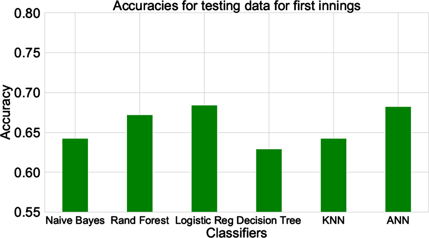
Fig. 13
Accuracies for different classifiers for testing dataset (for 2nd innings).
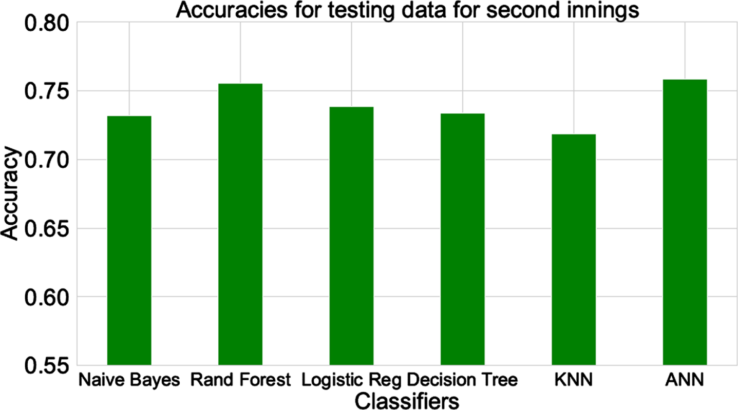
From Fig. 12 we conclude that the testing accuracies for the first innings lie in the range of about 63% (for decision tree) to about 68% (for logistic regression and ANN). In the second innings (Fig. 13) the prediction accuracies improve, and lie in the range of 72% (for k-NN) to 76% (for random forest and ANN). This improvement can be attributed to availability of more match specific data while making the second innings predictions (the first innings performance of the match under consideration is also included now). Random forest, logistic regression, and ANN are the best three classifiers for both the innings. Similar performances of different classification techniques in a given innings demonstrate that the predictive strength lies in the features rather than the classification technique(s).
6.2State by state prediction
Figures 14 and 15 present the state-by-state or in-play prediction accuracies for various classifiers for both the innings. As also concluded from Section 6.1, random forest, logistic regression, and ANN classification techniques are the best three performers in the first innings (Fig. 14). In the initial states of the first innings, the in-play prediction accuracy is about 62% for these three classifiers, which improves up-to 70% in the later states. The performance of all the classifiers is almost similar in the second innings (Fig. 15), with the prediction accuracy improving from 65% in the initial states to about 85% in the later states. The general trend is that as the match progresses, and we get more and more match data, the in-play prediction accuracy improves. In other words, as we get more match data and reach closer towards the end of the match, the uncertainty about the final result reduces which leads to better prediction. This trend is more prominent in the second innings than the first innings which leads to the conclusion that the deciding phase of the match lies in the second innings. Also, by the second innings, we get the understanding of the batting and bowling performance of both the teams; hence, uncertainties due to external factors (which affects both the teams equally) get resolved by this time. These factors include batting/bowling friendly pitches, seaming/turning pitches, ground size, etc.
Fig. 14
Over by over in-play prediction accuracies of different classifiers for the testing dataset (for 1st innings).
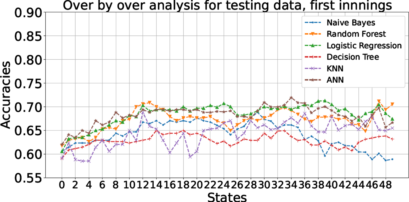
Fig. 15
Over by over in-play prediction accuracies of different classifiers for the testing dataset (for 2nd innings).
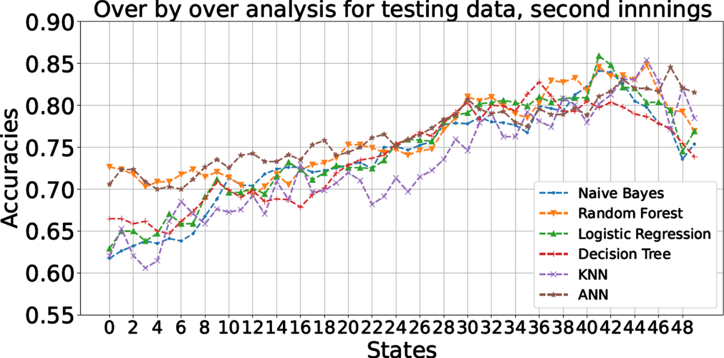
Figure 15 shows that the prediction accuracy is maximum around the 43rd state of the second innings, and reduces afterwards (against the otherwise increasing trend) in the so-called slog/death overs. We believe that the following factor contributes to this behavior: The matches which have clear winners (either because of the difference in the team quality, or because one of the teams performed very well on the given day), would finish by this state. Hence, only the ‘closely contested matches’, which can go either way, would be continuing beyond this state. These matches may remain unpredictable until the very last ball because of the unpredictable hitting ability of a batsman, or the uncertain wicket-taking ability of a bowler in the death overs. Thus, the winner is more uncertain for such states, leading to difficulties in prediction, and hence a lower classification accuracy.
The prediction accuracy does not have a smooth increasing trend as the states progress. This is partially because the number of data points vary for each state—recall that if a match finishes early, it would not contribute to the data for states beyond which the match finished. In addition, the winning prospect of a team does not always swing in one direction monotonically. The performance (runs scored, wickets falling, etc.) of each team fluctuates from state to state. Since there is only a limited pool of data of the ODI matches, these fluctuations cannot be averaged out completely.
6.3Comparison with the past literature
Past results are not directly comparable with our work mainly because of the differences in the datasets used and the prediction framework employed. Moreover, some of the past literature on ODI matches make a static prediction of the winner at the beginning of the innings, which is not the case for our work. However, Table 3 presents the accuracies reported in the previous literature for the ODI matches. Our framework seems to obtain better accuracies than the ones employed in the previous literature.
Table 3
Comparison of the present work with the past literature on ODI winner prediction
| Literature | Dataset description | Reported accuracy |
| Bailey and Clarke (2006) | 100 ODI matches played in 2005 | 71% |
| Sankaranarayanan et al. (2014) | 125 ODI matches played among top 9 teams from January 2011 to July 2012 | 68% –70% |
| Jhanwar and Pudi (2016) | 366 ODI matches played among top 9 teams from 2010 to 2014 | 59% –70% |
| Our work | 1359 ODI matches played among top 10 teams from January 2004 to January 2022 | 63% –76% (aggregated, Figs. 12 & 13) 60% –85% (in-play, Figs. 14 & 15) |
7Explainable AI: What has the model learned?
Recently, researchers have made a lot of progress in developing tools to explain the machine learning models. Methods like neural network, random forest, etc. behave as a black box model, and do not explain why a certain prediction is produced. To alleviate this, explainable AI techniques were developed. Explainability increases the trust of human users on the machine learning models because one can identify biases a model might have (unintentionally) incorporated, or if the model is learning correct parameters. Standard techniques for explainable AI include SHAP, developed by Lundberg and Lee (2017), and LIME, developed by Ribeiro et al. (2016). In the present work we use the SHAP framework which is based on the Shapley values concept from cooperative game theory (Winter, 2002). Specifically, we use the tree explainer of the SHAP package implemented in Python language to explain the results of the random forest classifier (Lundberg, 2023). We get a SHAP score for each feature of a given test point. We compute the mean of the magnitude of these SHAP values for all test points in a given state, and plot the results in Figs. 16 and 17 for both the innings. Higher mean value indicates that the model has placed more importance on that particular feature to make the prediction in that state.
Fig. 16
SHAP scores for the testing dataset for all the states (for 1st innings).
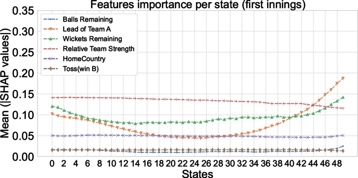
Fig. 17
SHAP scores for the testing dataset for all the states (for 2nd innings).
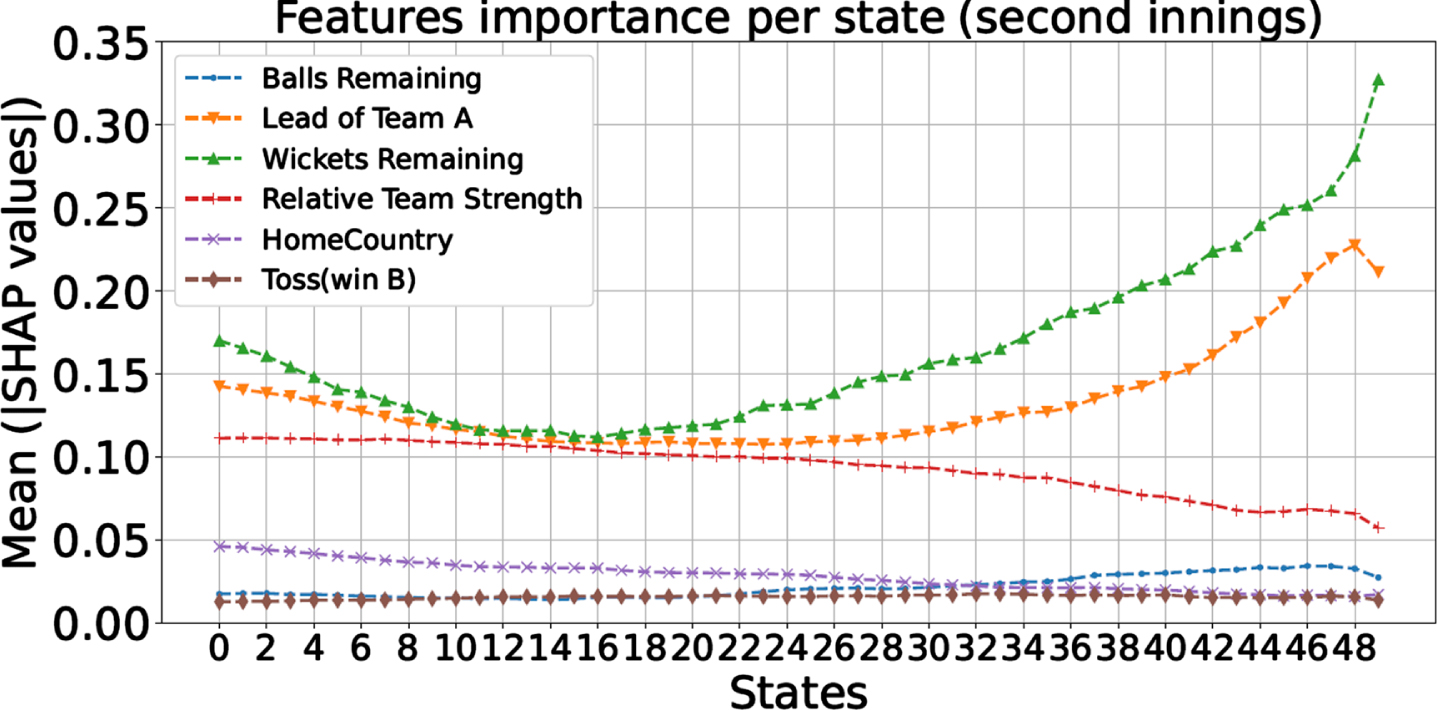
Plots in Figs. 16 and 17 demonstrate the following:
1. In the initial phase of the first innings, since there is little information about the current status of the match, ‘relative team strength’ is the most important feature to contribute to the model decision. Its importance keeps decreasing throughout the first and the second innings as we collect more information about the match status.
2. Next to the ‘relative team strength’, the features capturing the match situation—‘wickets remaining’ and the ‘lead of team A’—play an important role in the powerplay overs2 of the first innings. Figure 16 shows that their importance slightly reduces in the middle overs compared to the powerplay overs. This means that the model is capturing the powerplay performance of the batting team to make the prediction. Sometimes, in the powerplay overs, the new ball swings and seams more than usual, providing the bowling team an increased opportunity to take wickets; whereas, in other cases, the batting team does exceedingly well. Generally, the teams play defensively in the middle overs—the batting team tries to conserve wickets, and the bowling team tries to limit the scoring opportunities, making the middle overs less exhilarating. Thus, the match situation features assume greater significance in the non-middle overs. This trend is also visible in the second innings (Fig. 17), with an additional observation that importance of the ‘relative team strength’ is lower than the match situation features since the very beginning of the second innings.
3. Generally, the batting team tries to accelerate scoring in the slog/death overs, which is the final part of the innings. Thus, we see the match situation features overtaking the relative team strength as the best predictor in the first innings (Fig. 16). In other words, the model captures the initiative of the batting team to change the momentum of the match, or the lack of it (by favoring the bowling team), in making the prediction. The trend—the importance of match situation features increases in the slog overs compared to the middle overs—is also visible in the second innings (Fig. 17) for similar reasons.
4. Among the features ‘toss’ and ‘home country’, the model uses the home country feature to a greater extent for the prediction. However, in the overall framework, these two features do not play a dominant role, more so in the second innings than the first innings.
5. Surprisingly, ‘balls remaining’, which also captures the match situation, does not seem to play a critical role as compared to the other two match situation features. The feature heatmaps for both the innings (Figs. 10 and 11) reveal that ‘balls remaining’ correlates strongly with the ‘lead of Team A’ and ‘wickets remaining’ (–0.93 and 0.75 in the first innings respectively; and, 0.74 and 0.75 in the second innings respectively). In addition, Figs. 4 and 7 show that, independently, the predictive strength of ‘balls remaining’ feature is low. Hence, the rest of the two match situation features (‘wickets remaining’ and ‘lead of Team A’) are being used as a proxy for ‘balls remaining’ feature, thereby reducing its SHAP score.
6. From the qualitative analysis of the box plots in Figs. 4 to 9 we can notice that, for label 0 and label 1, difference in distribution of data is greatest for ‘wickets remaining’, followed by the ‘lead of Team A’, and least for ‘balls remaining’. The SHAP scores in Figs. 16 and 17 quantitatively capture the same trend by assigning the highest score to ‘wickets remaining’, followed by the ‘lead of Team A’, and least to ‘balls remaining’ (among these three dynamic features for a majority, if not all, of the states). It is satisfying to know that the model is emphasizing correct features to make a decision.
To summarize, the importance of the match situation features keeps increasing and the importance of the ‘relative team strength’ keeps decreasing, in making the predictions as the match progresses.
8Conclusions
In this work we have presented a framework for in-play winner prediction of a cricket ODI match. The contest is divided into 50 states for each innings, and a prediction is made in each of these states based on the static and evolving/dynamic match data. We train a machine learning model with six features to achieve this goal. Three of the six features are fixed throughout the match (static features)—relative team strength, home country, and winner of the toss. Rest of the three features depend on the current state of the match (dynamic features)—wickets remaining, lead of Team A, and balls remaining. The results are presented on a dataset of completed 1359 men’s ODI matches played between January 2004 to January 2022.
We analyzed the dataset and demonstrated the predictive strength of the six features. Further, we used multiple classifiers for an in-play winner prediction task and obtained the best in-play prediction accuracy of about 70% in the first innings, and about 85% in the second innings. As the match progresses, the prediction accuracy improves until the death overs of the second innings, where it starts to decrease due to uncertainties in the closely contested matches.
We also employed explainable AI techniques to analyze and interpret the working of the machine learning models. The insight gained was that the static features contribute more to the predictions at the initial phases of the match, but as the match progresses, the dynamic features assume increasing importance. Our work finds applications in preparing tools for in-play winner prediction that can be used in sports websites and mobile applications, providing analytics during live television commentary, legal betting platforms, etc.
Notes:
1. For example, in a day match, if it is overcast and the ball is likely to swing, the team winning the toss may elect to bowl first. The same is true if the venue is known to have dew in the evening (which hurts the bowler’s grip) in a day/night match.
2. The initial 10 overs of both the innings have a field restriction that only 2 fielders are allowed outside the 30 yards circle. The exact rules of the powerplay have changed over the years.
References
1 | Bailey M. , Clarke S.R. (2006) , Predicting the match outcome in one day international cricket matches, while the game is in progress, Journal of Sports Science & Medicine, 5: (4), 480–487. https://pubmed.ncbi.nlm.nih.gov/24357940/ |
2 | Berrar D. , Lopes P. , Dubitzky, W. (2019) , Incorporating domain knowledge in machine learning for soccer outcome prediction, Machine Learning, 108: , 97–126. https://doi.org/10.1007/s10994-018-5747-8 |
3 | Boehmke B. , Green well B. 2019, Hands-on machine learning with R. Chapman and Hall/CRC. |
4 | Chen M.Y. , Chen T.H. , Lin S.H. (2020) , Using Convolutional Neural Networks to Forecast Sporting Event Results, Deep Learning: Concepts and Architectures, 866: , 269–285. https://doi.org/10.1007/978-3-030-31756-0_9 |
5 | Daud A. , Muhammad F. , Dawood H. , Dawood H. (2015) , Ranking cricket teams, Information Processing & Management, 51: (2), 62–73. https://doi.org/10.1016/j.ipm.2014.10.010 |
6 | Davoodi E. , Khanteymoori A.R. (2010) , Horse racing prediction using artificial neural networks, Recent Advances in Neural Networks, Fuzzy Systems & Evolutionary Computing, 2010: , 155–160. |
7 | Duckworth F.C. , Lewis A.J. (1998) , A fair method for resetting the target in interrupted one-day cricket matches, Journal of the Operational Research Society, 49: (3), 220–227. https://doi.org/10.1057/palgrave.jors.2600524 |
8 | Jhanwar M.G. , Pudi V. 2016, Predicting the Outcome of ODI Cricket Matches: A Team Composition Based Approach, In MLSA@ PKDD/ECML. |
9 | Kaluarachchi A. , Aparna S.V. 2010, CricAI: A classification based tool to predict the outcome in ODI cricket, In 2010 Fifth International Conference on Information and Automation for Sustainability (pp. 250-255). IEEE. https://doi.org/10.1109/ICIAFS.2010.5715668 |
10 | Kamble A.G. , Rao R.V. , Kale A. , Samant S. (2011) , Selection of cricket players using analytical hierarchy process, International Journal of Sports Science and Engineering, 5: (4), 207–212. |
11 | Liu G. , Schulte O. 2018. Deep reinforcement learning in ice hockey for context-aware player evaluation, In Proceedings of the 27th International Joint Conference on Artificial Intelligence (pp. 3442-3448). https://doi.org/10.24963/ijcai.2018/478 |
12 | Lundberg S.M. , Lee S.I. 2017, A unified approach to interpreting model predictions, Advances in Neural Information Processing Systems, 30. |
13 | Morley B. , Thomas D. (2005) , An investigation of home advantage and other factors affecting outcomes in English one-day cricket matches , Journal of Sports Sciences, 23: (3), 261–268. https://doi.org/10.1080/02640410410001730133 |
14 | Muazu Musa R. , Abdul Majeed, PPA. , Taha Z. , Chang S.W. , Ab. Nasir, A.F. , Abdullah M.R. (2019) , A machine learning approach of predicting high potential archers by means of physical fitness indicators, PLoS One, 14: (1), e0209638. https://doi.org/10.1371/journal.pone.0209638 |
15 | Mukherjee S. (2014) , Quantifying individual performance in Cricket—A network analysis of Batsmen and Bowlers, Physica A: Statistical Mechanics and its Applications, 393: , 624–637. https://doi.org/10.1016/j.physa.2013.09.027 |
16 | Owramipur F. , Eskandarian P. , Mozneb F.S. (2013) , Football result prediction with Bayesian network in Spanish League-Barcelona team, International Journal of Computer Theory and Engineering, 5: (5), 812–815. https://doi.org/10.7763/IJCTE.2013.V5.802 |
17 | Passi K. , Pandey N. (2018) , Increased prediction accuracy in the game of cricket using machine learning, International Journal of Data Mining & Knowledge Management Process, 8: (2), 19–36. |
18 | Perera H. , Davis J. , Swartz T.B. (2016) , Optimal lineups in Twenty20 cricket, Journal of Statistical Computation and Simulation, 86: (14), 2888–2900. https://doi.org/10.1080/00949655.2015.1136629 |
19 | Rahman M.M. , Shamim M.O.F. , Ismail S. 2018, An analysis of Bangladesh one day international cricket data: a machine learning approach, In 2018 International Conference on Innovations in Science, Engineering and Technology (ICISET) (pp. 190-194). IEEE. https://doi.org/10.1109/ICISET.2018.8745588 |
20 | Ribeiro M.T. , Singh S. , Guestrin C. 2016, “Why should I trust you?” Explaining the predictions of any classifier, In Proceedings of the 22nd ACM SIGKDD international conference on knowledge discovery and data mining (pp. 1135-1144). https://doi.org/10.1145/2939672.2939778 |
21 | Roy S. , Dey P. , Kundu D. (2017) , Social network analysis of cricket community using a composite distributed framework: From implementation viewpoint, IEEE Transactions on Computational Social Systems, 5: (1), 64–81. https://doi.org/10.1109/TCSS.2017.2762430 |
22 | Sankaranarayanan V.V. , Sattar J. , Lakshmanan L.V. 2014, Auto-play: A data mining approach to ODI cricket simulation and prediction, In Proceedings of the 2014 SIAM international conference on data mining (pp. 1064-1072). Society for Industrial and Applied Mathematics, https://doi.org/10.1137/1.9781611973440.121 |
23 | Viswanadha S. , Sivalenka K. , Jhawar M.G. , Pudi V. 2017, Dynamic Winner Prediction in Twenty20 Cricket: Based on Relative Team Strengths, In MLSA@ PKDD/ECML (pp. 41-50). |
24 | Wang Y. , Liu W. , Liu X. (2022) , Explainable AI techniques with application to NBA gameplay prediction, Neurocomputing, 483: , 59–71. https://doi.org/10.1016/j.neucom.2022.01.098 |
25 | Winter E. 2002, The Shapley value, Handbook of Game Theory with Economic Applications, 3, 2025-2054. https://doi.org/10.1016/S1574-0005(02)03016-3 |
26 | ESPN Cricinfo. 2023, ESPN Cricinfo, ESPN Sports Media Ltd. Available at: https://www.espncricinfo.com (Accessed: March 19, 2023). |
27 | International Cricket Council. 2023, International cricket council: ICC Development. Available at: https://www.icccricket.com/about/development (Accessed: March 19, 2023). |
28 | Lundberg S. 2018, SHAP:Welcome to the SHAP documentation. Available at: https://shap.readthedocs.io/en/latest/ (Accessed: March 19, 2023). |
29 | Media Infoline. 2018, IFSG-AC Nielsen: 2 out of 3 online cricket fans are aware of fantasy sports in India, Media Infoline. Available at: https://www.mediainfoline.com/article/ifsgac-nielsen-2-online-cricket-fans-aware-fantasy-sports-india (Accessed: March 19, 2023). |
30 | Rushe. 2023, Cricsheet. Available at: http://cricsheet.org (Accessed: March 19, 2023). |
31 | Smith T. 2023, How popular is cricket around the world? SQaF. Available at: https://sqaf.club/how-popular-is-cricket/ (Accessed: March 19, 2023). |

