Parametric modeling and analysis of NFL run plays

1Introduction

The NFL has seen offensive development explode over the last several decades, seeing yards per game increase from 295 for an average team in the 1970s to 347 in the 2010s (Gough, 2022). With this much change, it is hard to imagine further room for improvement, and therefore identifying factors that can fundamentally improve a team’s performance should prove to be a difficult task. The question of how to improve a team no longer has surface level answers and the use of high level data analysis to inform decisions is, we argue, a necessary next step to seriously consider.

In Biro and Walker (2022), a step towards a data driven decision theoretic approach to play calling was made by establishing a method for an optimal play calling policy. The techniques relied heavily on the probability transition function that dictates how states transition from one to another given a specified action. A state here is represented by a down, a yardage to go to secure a first down, and the line of scrimmage.

The probabilities are estimated from data. At an average level; i.e. over all football teams in the NFL, a nonparametric estimator works. There is sufficient data for all the states to get a good estimation of the probabilities of outcomes following choices of play. However, when we wish to look at team specific outcomes, data is more sparse, and hence parametric models become essential. Provided the model parameters are interpretable, the change in estimated parameters for different teams can lead to an understanding of what activities/decisions the teams are making which determines how well a team does. This is an ambitious endeavour and yet we believe we have found some significant criteria in team choices which explains to some extent team offensive proficiencies, specifically relating to run plays.

Consequently, this paper details the modeling methods used for creating accurate probability transition distributions for run plays. Additionally, we provide insight on some of the interpretable outcomes of the parameters. We attempt to answer the question: “What makes a good running football team?" using information that can be gleamed from the parameters identified in the modeling efforts.

Much of the current literature regarding the modeling of run plays originated in the 2020 Big Data Bowl, where individuals were tasked with predicting the amount of yards gained using player tracking data. These projects proved fruitful, identifying many features of a successful running game, such as a ball carrier’s effective acceleration (Ploenzke, 2019), the initial open space generated by offensive linemen (Stern, 2019), and field control generated by each team’s positioning (Brighenti, 2019). However, each of these projects rely on tracking data and therefore provide limited insight on the ability to advise decisions in real time, due to the fact that data is not available until the end of the play (or more realistically until after the game). Moreover, NFL and NCAA teams (at the time of writing) are prohibited from accessing computers during the game, and although it may be possible that this restriction is lifted in the future, tracking data still would not be a particularly helpful pre-play predictive tool because of the uncontrollable nature of the opponents’ actions. Therefore, the measures created are better suited for descriptive evaluation metrics, while the methods proposed in this paper will focus on generating probability densities that can inform in game decisions using available online information. Additionally, these aforementioned projects tended to focus on evaluation at the player level. The results of this paper will take a higher level approach to improving the run game of a team.

Previous work using NFL play by play data has focused on two topics: creating descriptive statistics and predicting play types. For the former, research into expected points and win probabilities have been exceptionally popular, implemented primarily in the work of Yurko et al. (2018) and Burke (2010a,b). These metrics have been widely accepted in the analytics community, using them as tools to understand decision making and to evaluate players. The latter has been explored by multiple groups (Lefort et al., 2022; Joash Fernandes et al., 2020), attempting to find models that successfully predict play calls. The scope of the work is directed towards adversarial strategy, attempting to find trends in decisions that can be used to help a defense prevent an offense from advancing.

The closest work to our own, we believe, was conducted in Lutz, and Kassarnig (2016), where play by play data was used to predict the number of yards gained (amongst other variables). These authors explored several different machine learning techniques, such as regression trees, support vector regression, and artificial neural networks, to predict a number of outcomes of interest using play by play data. However, their methods used information not available at the start of the play (such as pass length and side of the field) in their predictions, whereas our research will focus on using only presnap information in order to provide prescriptive decisions. Additionally, their work created point estimators for yards gained, whereas our results will provide distributions of all possible events.

Central to our paper is the modeling of the yards gained outcome following the choice to run for an NFL team. This will be formulated using a regression model where the features are line of scrimmage, yards to first down, and down number. These were successfully assumed to be the key features from Biro and Walker (2022). The key model is the skew–t distribution, which we claim provides a good fit for the data and allows us to separately model important aspects of a distribution; i.e. the mean, the variance, the skewness and the heaviness of tail. The skew–t model is described in detail in section 2. In section 3 we indicate how we analysed the data and present the raw results. Our analysis of the results is to be found in section 4 and section 5 concludes with a discussion.

2Modeling

At each state, which we have indicated is the triple down, line of scrimmage and yards to a first down, we adopt the idea that there are four actions a team can choose from: a run, a pass, a punt, or a field goal attempt. For each state-action pairing, our goal is to model the probability of outcomes which is tantamount to estimating the transition probabilities from state to state. In this paper, we will focus exclusively on the modeling of run plays. First we will begin by modeling the population; i.e. all the teams in the league, and then model the team adjustments. Such a model would be known in the statistical modeling community as a random effects model.

2.2The Skew-t distribution

The family of distributions used to model the data is provided by the skew–t distribution, as defined in Arellano-Valle and Azzalini (2013). The density function is given by:

(1)

f(y;ξ,ω,α,ν)=2ωt(z;ν)T(αzν+1ν+z2;ν+1),wherez=y-ξω.       

Here t and T represent the Student–t density and distribution, specifically

(2)

t(z;τ)=Γ(τ+12)τπΓτ2)(1+x2τ)-τ+12

(3)

T(z;τ)=12+xΓ(τ+12)×2F1(12,τ+12;32;-x2τ)πτΓ(τ2),

where Γ (·) is the gamma function and ₂F₁ (·) is the hypergeometric function.

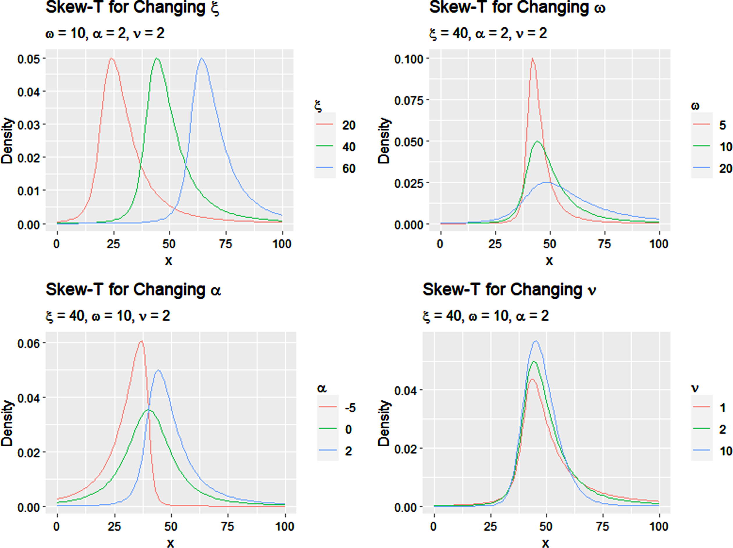
The skew–t distribution has four parameters: (ξ, ω, α, ν). These parameters can be understood broadly as (but not fully separately from a mathematical point of view) as mean, variance, skewness, and degrees of freedom, which controls the heaviness of the tails. Figure 1 shows a few examples of the skew-t density evaluated for changing values of each parameter. As can be seen in the images, the ξ parameter shifts the location of the mode, the ω parameter has a large influence over the spread of the distribution, the α parameter influences the symmetry and skewness of the distribution, and the ν parameter controls the size of the tails. Each of the parameters also has some influence over other effects; for example, increasing ω changes the spread but also slightly shifts the mode. However, we will use the terms mean, variance, skewness, and degrees of freedom, aka kurtosis, interchangeably with their respective parameters for ease of discussion.

Fig. 1

Plots of skew-t densities for changing parameter values.

This distribution displays smooth, unimodal behavior, with parameters that allow for relative control over the occurrence of extreme and one-sided events. We observe similar structure in the distribution of run plays, and therefore believe the skew-t distribution is a good choice as a parametric model for the data.

2.3Goodness of fit

Following the aforementioned theme, here we statistically assess the fit of a skew-t distribution for the data. While a visual inspection shows the model fits the data well, a statistical test for fit is necessary. However, it is infeasible to evaluate the goodness of fit for all states, and therefore we will consider the most common state; namely a 1st and 10 on the offensive team’s own 25 yard line; i.e. DOWN = 1, DIST = 10, LOS = 75. This state represents where a team obtains the ball after a kickoff touchback (amongst other options), and therefore is the most common state, with 1555 plays. We remove the six touchdown outcomes, for reasons that will be elaborated on in proceeding sections, leaving n = 1549 non–touchdown plays with the amount of yards gained spanning -9 to 70 yards. Figure 2 shows this data fit with the corresponding skew-t model. The specific density is obtained by minimizing the objective function over (ξ, ω, α, ν);

∑y=-970{Fn(y)-F(y|ξ,ω,α,ν)}2Fn(y),

where F_n (·) is the empirical cumulative distribution function for yards gained evaluated at y and F (·) represents the cumulative distribution function of the skew-t.

Fig. 2

Skew-t fit for most common state, with the histogram bars indicating the amount of yards gained on observed plays and the black line indicating the predictive density.

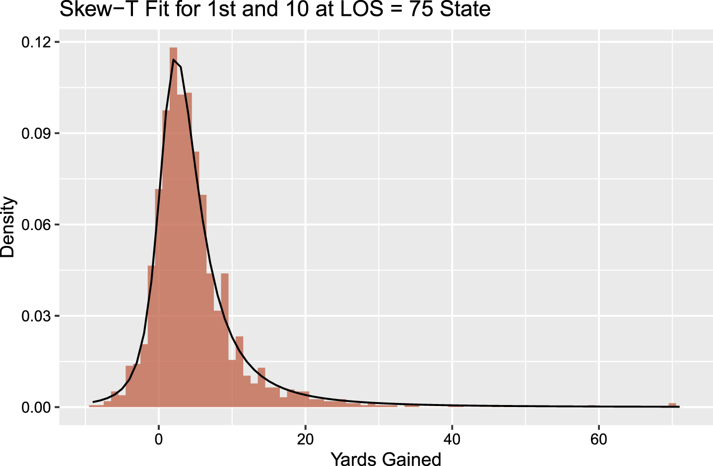
Using Pearson’s χ-squared goodness of fit test (Pearson, 1900), we obtain a test statistic value of 83.46. For df = 80, this corresponds to a p-value of 0.374, and hence there is no reason to reject the hypothesis that the data arose from a skew–t distribution. Performing a test for all states is not appropriate; smaller sample sizes and the play of chance in the testing procedure would not lead to a 100% fit. Nothing seen or checked would suggest the skew-t is not suited for the modeling of the data.

2.4League average run modeling

The nature of run plays is smooth, with yards gained typically having a unimodal distribution with a single heavy tail on the positive part. We choose to build a Bayesian model around a skew-t likelihood. The skew-t distribution is truncated at each end to represent the constraints of the game limiting the yards gained to a touchdown on the positive part and a safety on the negative part. Additionally, the skew-t is mixed with a point mass probability of scoring a touchdown; since touchdown scoring events tend to happen with higher frequency than other heavy tail events. Not including this point mass for touchdowns would result in an overcorrection of the parameters to fit the heavy tail of the skew-t, and therefore separating these points allows for more accurate fits. We do not observe the same behavior in the negative part, and therefore do not include a point mass for safety plays.

To incorporate state information, the parameters of the skew-t distribution and the point mass probability are formed as linear combinations of the down, distance, and line of scrimmage with parameters estimated via Markov chain Monte Carlo simulation. The following set of equations represents the skew-t mixture model used for the modeling of yards gained, denoted by y_i for play i and with state x_i:

(4)

p(yi|xi,β,wi)=wiF(yi|ξi,ωi,αi,νi)1[yi∈(LOSi-100,LOSi]]+(1-wi)1[yi=LOSi]        

(5)

ξi=βINTξ+∑d=14βDOWN=dξ1[DOWNi=d]+βDISTξDISTi+βLOSξLOSi        

(6)

logωi=βINTω+∑d=14βDOWN=dω1[DOWNi=d]+βDISTωDISTi+βLOSωLOSi        

(7)

αi=βINTα+∑d=14βDOWN=dα1[DOWNi=d]+βDISTαDISTi+βLOSαLOSi        

(8)

logνi=βINTν+∑d=14βDOWN=dν1[DOWNi=d]+βDISTνDISTi+βLOSνLOSi        

with the prior for all the β parameters are independent normal with zero mean and a large variance, and w_i ∼ Beta (19 + n_i,ST, 1 + n_i,TD). Here

ni,j=∑i=1N1[di=j],

where d_i = ST, ST = coming from the skew–t, with probability

P(di=ST)=wiF(yi|ξi,ωi,αi,νi)1[yi∈(LOSi-100,LOSi]]wiF(yi|ξi,ωi,αi,νi)1[yi∈(LOSi-100,LOSi]]+(1-wi)1[yi=LOSi]

and d_i = TD with probability 1 - P (d_i = ST). The ω_i and ν_i parameters are modeled on log scale to ensure positivity. Thus, the task of identifying the probability distribution for yards gained on a run play comes down to estimating the parameters β=βCOVθ , for each combination of COV ∈ {INT, DOWN = 1, DOWN = 2, DOWN = 3, DOWN = 4, DIST, LOS} and θ ∈ {ξ, ω, α, ν}, along with the point mass weight parameters w_i.

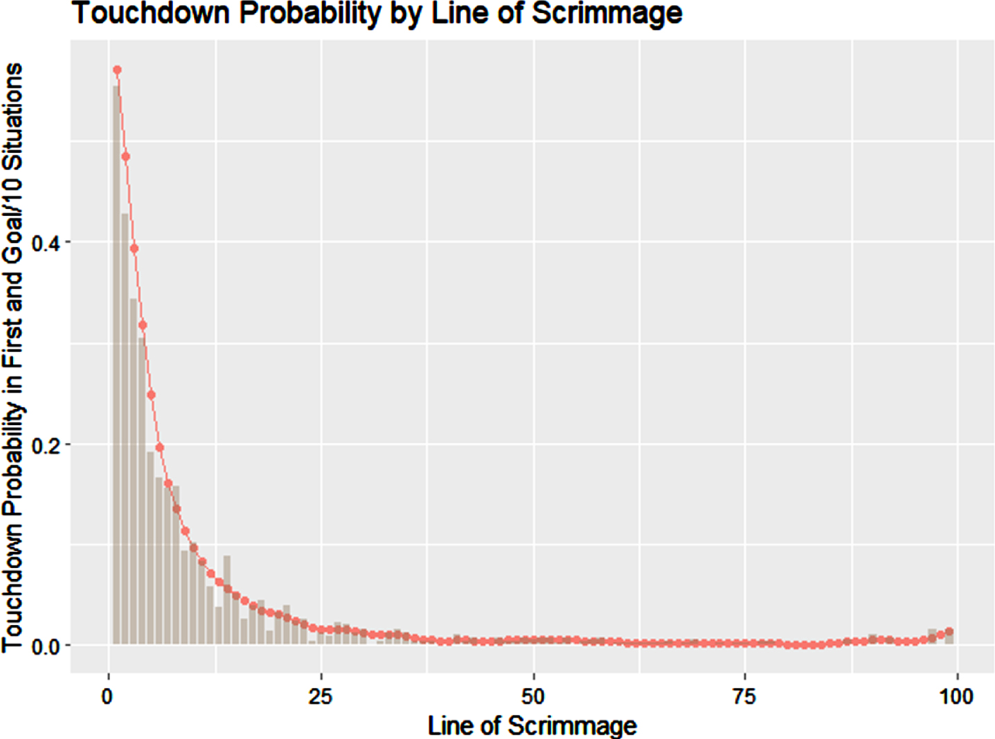
We consider the d_i to be latent labels of each of the plays as coming from either the skew-t distribution or the point mass distribution. For all plays that do not result in touchdowns, d_i is deterministic as a standard play (ST). However, for touchdown plays, there is a high (but not 100%) probability that d_i = TD. This mixing gives the interpretation of allowing for the total touchdown probability to be a combination of gaining exactly LOS_i yards coming from the skew-t distribution plus the probability of more yards that could be gained had the yards gained not been truncated by the touchdown, represented by 1 - w_i. Additionally, we have chosen to smooth the (w_i) values using a rolling average filter (K = 2, two-sided) to create a smooth representation of the touchdown probabilities, removing the effects of outliers at specific yard lines. Figure 3 shows the touchdown probabilities (for 1st and goal or 1st and 10 for LOS > 10) plotted against the respective frequency at that yard line.

Fig. 3

Modeled probability of scoring a touchdown versus empirically observed touchdown probability for 1st and 10 scenarios, or 1st and goal scenarios for LOS less than 10.

This model yields results both accurate and interpretable. With n = 19881 plays and 28 parameters to fit (with 99 (w_i) parameters that are nearly independently fit from the βCOVθ ), each parameter has a sufficient amount of plays that can be used to inform its value. The components of this model are a composition of standard approaches for Bayesian mixture models, with the added novel component of the skew-t distribution to account for the nature of run plays. The model assumes that the distribution of yards gained on a run play is dictated by the βCOVθ terms. Each of the individual βCOVθ parameters (excluding the βDOWNθ terms) are modeled assuming a linear relationship between the skew-t parameters and the state information. For example, incrementing DIST_i by one implies the ξ parameter will increment by βDISTξ . We assumed the relationship between DOWN_i and the skew-t parameters would likely be far from linear, as the difference in the distributions between 1st and 2nd plays is not similar to the difference between 2nd and 3rd down plays. Treating this relationship as linear would imply an equal shift in parameters for all values of DOWN_i, therefore we instead chose to treat DOWN_i as a categorical variable, giving each value its own βDOWNθ . We assumed no interaction effects between covariates, assuming a change in one covariate does not affect another covariate’s relationship with the parameters. This assumption tends to seem fair for most situations, as the observed data only changes slightly from state to state and therefore a more complex model would only provide marginal accuracy improvements at the cost of computational burdens and intuitive explanations.

2.5Team adjusted run modeling

Given the estimated parameters for the league average data, we can now identify trends at the team level. To make team adjustments, the model is an extension which allows for team additive shifts from the average values as follows:

p(yi|xi,βTeamθ,βCOVθ,wi)=wiF(yi|ξij,ωij,αij,νij)1[yi∈(LOSi-100,LOSi]]+(1-wi)1[yi=LOSi]

with

ξij=ξi★+βTeam=jξ,   ωij=ωi★+βTeam=jω,   αij=αi★+βTeam=jα,   νij=νi★+βTeam=jν,

where j is an indicator for the team. Here, the (ξi★,ωi★,αi★,νi★) represent the average parameters of the league model. Additionally, the (x_i) now contain information indicating the team.

These values were identified using a weighted MLE approach, where the weights were assigned according to the team’s run frequency for each state component relative to the league average frequency. This weighting was used to counter the effects of team specific trends for running in situations significantly more or less than the league average and to force the parameters to be a function of the team’s proficiency rather than their usage rate in a particular area. Team effects were computed over the entire two-year sample, acknowledging that coaching and roster turnover would naturally result in differing parameters from year to year, but are likely small changes in comparison to the effects of controlled covariates. Note that the values of βCOVθ and w_i do not need to be recomputed.

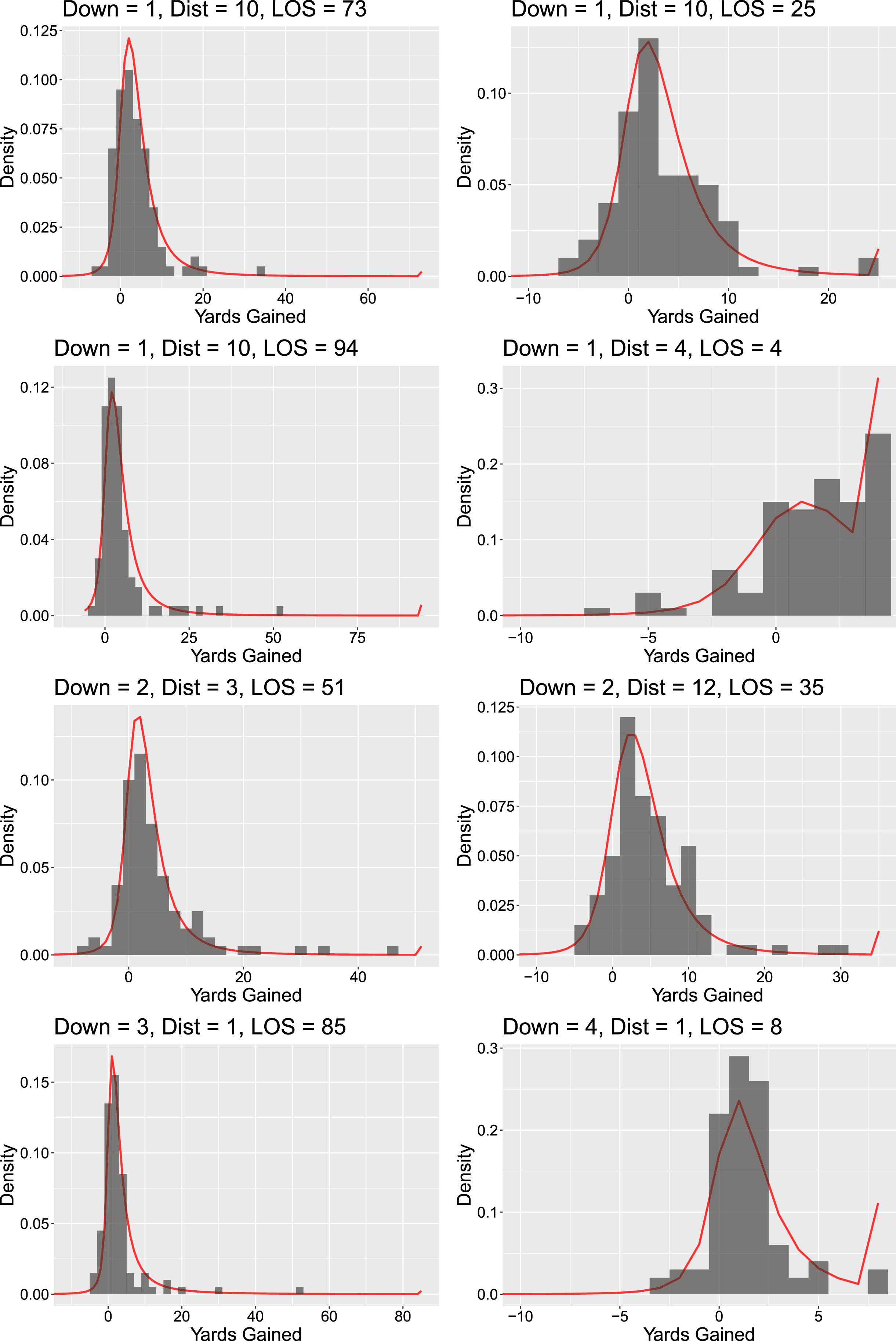
Fig. 4

Several examples of randomly chosen predictive distributions for run plays for a specific state, with observed data from similar states shown in histograms. Distributions have been truncated at -10 yards gained to expand images.

3Results

3.2Team model results

Table 1 shows the parameter values obtained for the team adjustments from the league average run model to create a team specific run model.

Table 1

Table of βCOVθ values after MCMC optimization. Values of COV are shown going down and values of θ are shown going across

βCOVθ	ξ	ω	α	ν
INT	-.777	1.508	2.909	1.221
DOWN = 1	.151	-.447	-1.291	-.104
DOWN = 2	.417	-.393	-1.423	-.022
DOWN = 3	.439	-.615	-1.221	-.336
DOWN = 4	.833	-.979	-1.664	-.363
DIST	.0553	.0257	-.0115	.0288
LOS	.00392	.00140	.00410	-0.00649

Similar to the coefficients in the league average model, we can interpret the individual effects of the team adjustment coefficients as well. For example, a negative βTeamξ value, as seen for teams like the Detroit Lions (DET), implies that the center of the skew-t has been shifted negatively from league average. This implies that holding all other parameters constant, the predicted mean yards per carry on comparable states would be lower for Detroit than the average team. However, this team also has a positive βTeamω adjustment, implying their spread of results is higher than the average team. This (holding βTeamα and βTeamν constant) indicates the team likely has a fairly boom or bust running game, perhaps with a small proportion of 4 to 6 yard gains, but more extreme results such as a 5 yard loss or 15 yard gain. This aligns with their results over the sample period. Interpretations such as these can be continued for the other parameters, providing insight into a team’s trends and proficiencies. To ensure the validity of these estimates, we created several plots of the predictive distributions, indicating a strong fit for each of the individual teams. Several of these plots have been included in Figure 5. Furthermore, we assessed goodness of fit under the skew-t distribution for the 1st and 10 from the team’s own 25 yardline state for each team. Figure 6 shows the distribution of p-values, showing no unexpected behavior as indicated by distribution appearing relatively uniform, as is assumed under the null hypothesis.

Fig. 5

Several examples of randomly chosen predictive distributions for run plays for a specific team for a specific state, with observed data from similar states for the team shown in histograms.

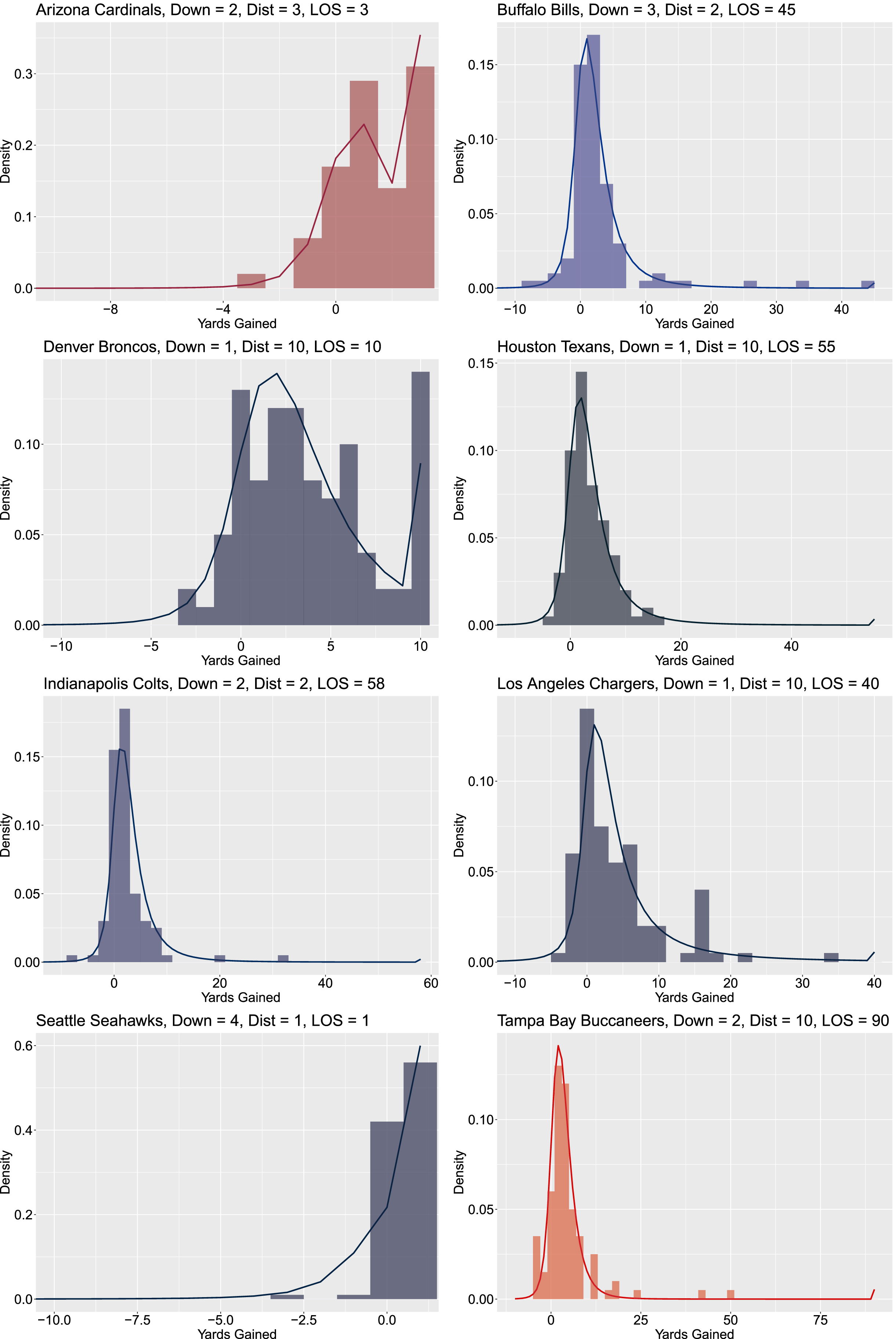
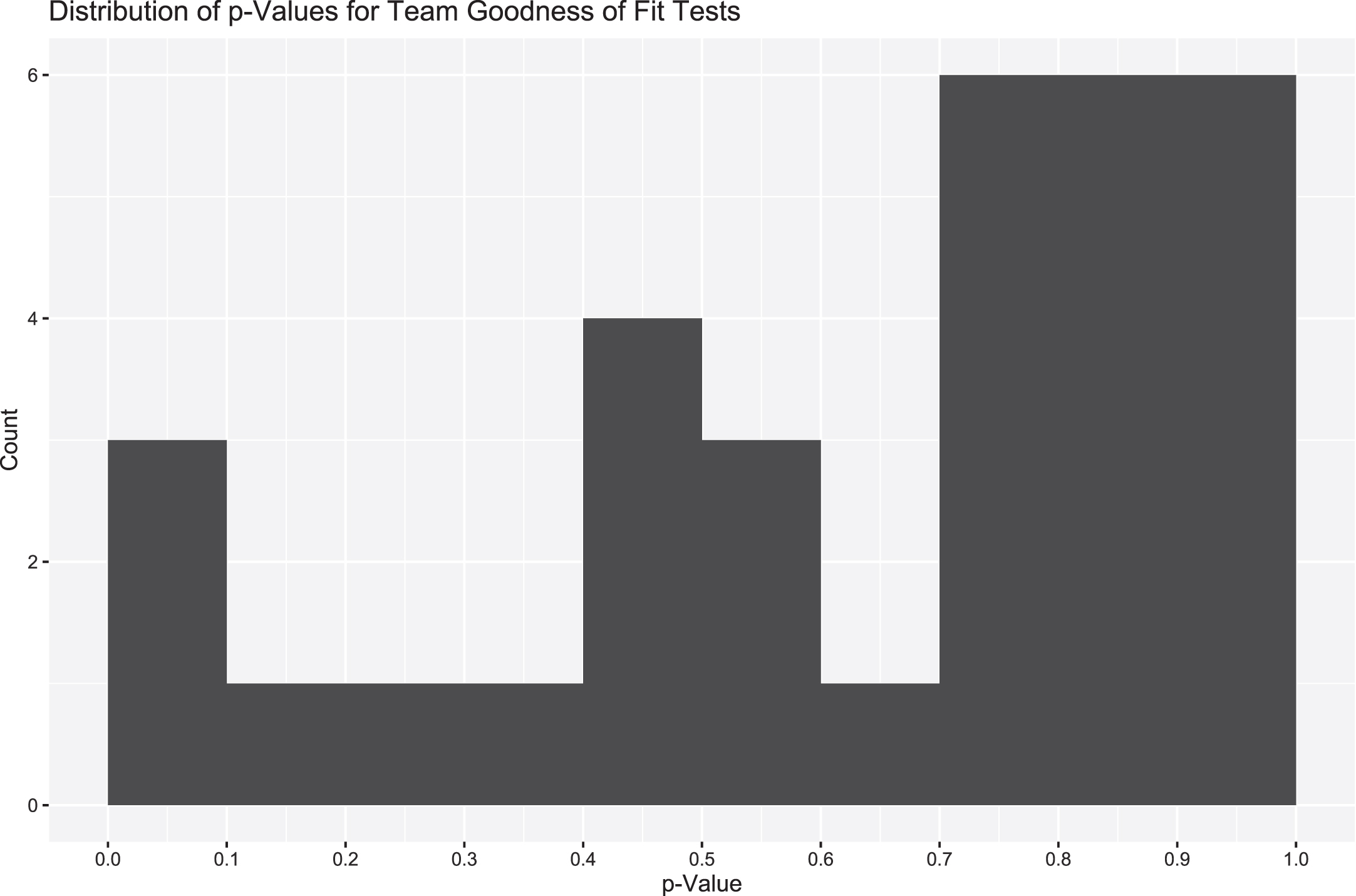
Fig. 6

Goodness of fit p-values for team parameters for 1st and 10 at their own 25 yardline state. Uniformity implies the skew-t remains a reasonable distribution with which to model to data.

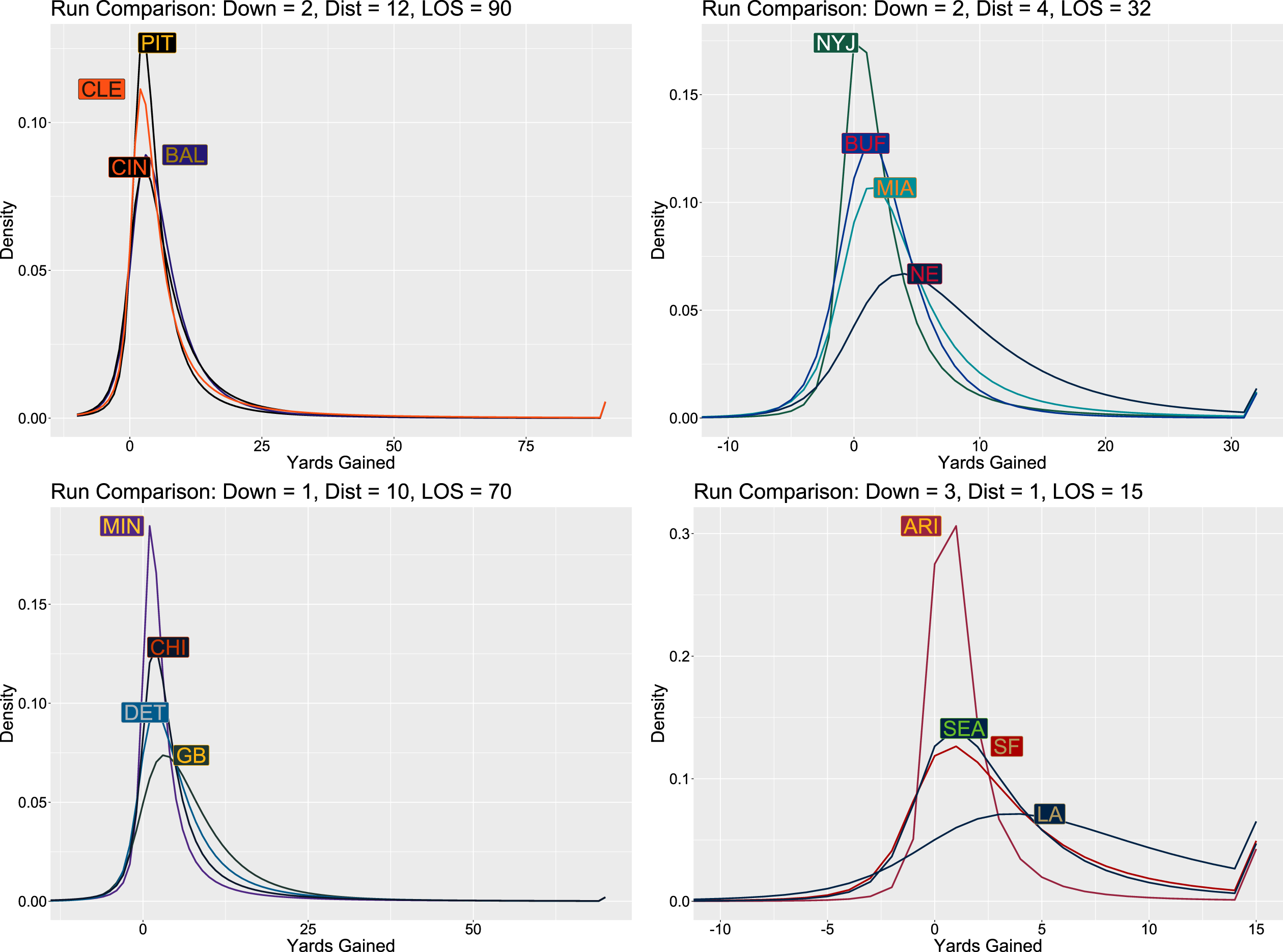
We also found it to be a fruitful task to compare the predictive distribution of run plays across the different teams to identify that we are able to distinguish between different team proficiencies and weaknesses. Figure 7 show a few different team predictive run distributions plotted against one another for identical scenarios. In these plots, one is able to compare the different properties of the predictive distributions for different teams in a visual manner. For example, one can see that the Los Angeles Rams (LA) has a heavier positive tail than the their divisional opponents (the NFC West), indicating they are more likely to have a larger gain than the Cardinals, Seahawks, and 49ers (ARZ, SEA, and SF). However the positive heavy tail has a cost, specifically by having a larger negative tail as well, indicating they also are more likely to have a run play for a loss. It is apparent that the predictive distributions are both proper fits for the individual teams and that they are useful in distinguishing trends at the team level.

Fig. 7

Comparison plots showing differences in predictive run distributions for different teams for a common state. Colors provided via R’s teamcolors package (Baumer and Matthews, 2020).

4Analysis

With these team adjustment parameters identified, we can examine them to identify what trends exist and correlate with successful run games. To do this, we created plots for each of the four sets of parameters against the team cumulative yards per carry over the two year dataset period. The choice to use yards per carry as the metric for effective rushing offense was chosen due to its simplicity in interpretation as well as its ability to avoid volume issues. Other metrics were checked to ensure consistency, such as EPA per run (Yurko et al., 2018), percentage of successful runs (Carroll et al., 1988), and each team’s ranking amongst the league for each of these statistics. All of these metrics have similar relationships with the parameters, and therefore we will proceed using yards per attempt. We will discuss a potential analysis that could be conducted using EPA/attempt, along with appropriate caveats, in Section 4.1.

Figure 8 shows these plots of the parameters against yards per attempt, where a relationship can clearly be seen between βTeamω (the variance parameter) and βTeamα (the skewness parameter) with the average yards per carry for each team in the period (correlations of -0.432 and -0.515 respectively). A test for significance for these correlations finds significant p-values for both parameters (p = 0.0135 and 0.00257 respectively). The relationships with βTeamξ (the center parameters) and βTeamν (the degrees of freedom parameters) were negligible, and therefore determined to have no meaningful relationship with running success.

Fig. 8

Parameters from team adjusted run model plotted against team yards per attempt, indicating a correlation between the high risk parameters and successful running teams.

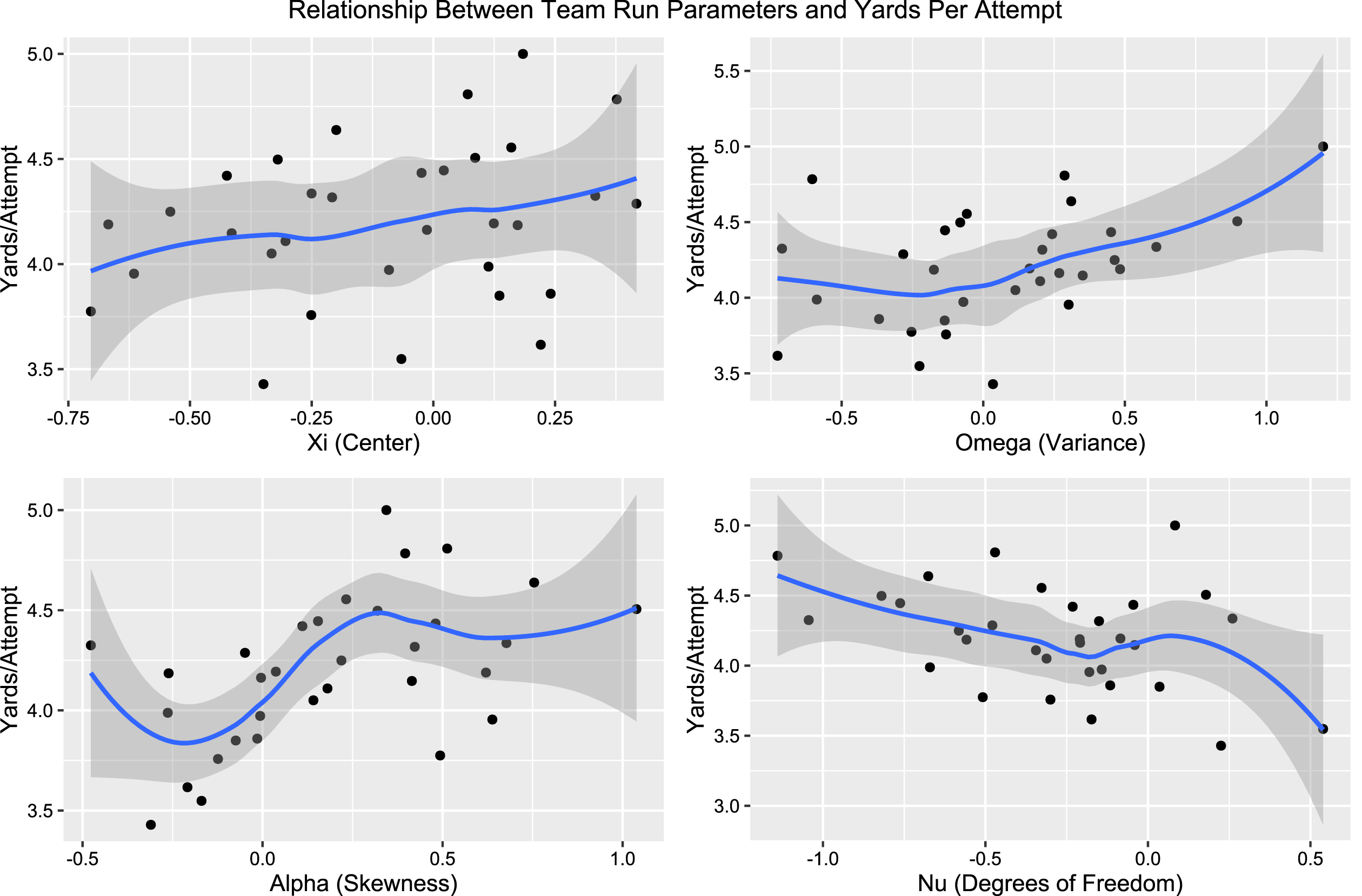
It is a usual phenomenon that high variance, and as a consequence higher skewness, while the mean is held fixed, indicates greater risk. Hence, the natural interpretation is to assume that the better rushing teams were willing to attempt more “high risk" run plays, implying that they are more likely to run the ball in a way that increase the probability of a nonsuccessful or even negative play in order to maximize their ability to generate a large run. It is well known that high variance has long been associated with high risk (Winterhalder, 2007; Coombs and Pruitt, 1960), and thus we will henceforth refer to high variance and skewness runs as high risk runs.

Consequently, there is something fundamental about the style of offense run by the successful teams that can be tied to high risk runs. One conjecture is that outside runs (regardless of the actual play scheme) are considered high risk runs. The idea of outside runs being more effective was partially studied in Seth (2020), but we plan on extending this analysis with a more directed approach employing the parametric regression skew-t model. The nature of an outside run requires the ball carrier to run towards the perimeter of the field prior to moving downfield to gain yards, implying that the risk of losing yards may be greater than a play where the ball carrier runs directly downfield. This higher risk of losing yards should also come with a higher chance of creating large gains, as moving outside may allow the back to avoid the larger potential tacklers (typically defensive linemen and linebackers) and may be more likely to induce a broken tackle from a smaller player (defensive backs). Therefore, we expect an outside run to have an association with high risk run activity.

We should make a clarification here of how we identify an inside or outside run. For the purposes of this paper, we will classify “outside" runs as plays where the run_gap column is marked as “tackle" or “end" according to the nflfastR labeling scheme (Carl and Baldwin, 2022). A visual inspection of the film of these runs show that these typically align with runs that are run to a gap located at least outside the guard (commonly referred to as the B gap), and are more commonly restricted to being outside the tackle (C gap) or even end (D gap). Additionally, the “run location" is marked as “left" or “right", as opposed to “middle", which seems to correspond nearly perfectly with “run gap" being labeled “NA", implying that the run is always “middle", “guard", “tackle" or “end". These runs being labeled as “outside" for our purposes encompass about 47% of all runs, with all other runs being labeled as “inside" runs.

It is also important to note that we recognize that a coach does not call “inside" or “outside" run as their play. While inside and outside zone run concepts exist, these concepts do not fully correspond to what we are labeling as inside and outside runs. The run is classified by an external source that is agnostic to the actual play calling scheme and is determined (by what it seems) solely by the final location of where the back runs. Any run scheme can be used in accordance with the findings of this paper, and therefore the results should be taken into consideration properly in order to determine how an individual team can adjust their scheme to be in line with more successful run behavior.

With these caveats in mind, we calculated the correlation between a team’s percentage of outside run plays called with the parameters of interest. Finding a correlation of.448 with the team variance parameter (and a slightly less interesting.323 correlation with the team skewness parameter), our hypothesis was supported by the moderate relationship. Furthermore, we conducted a test of significance to determine whether the relationship is statistically significant. Using a significance level of 5%, we performed a hypothesis test for the regression slope of percentage of outside runs. To account for the bounded nature of the percentage of outside runs statistic, we converted the value to the log odds of percentage of outside runs and used it as a covariate in a linear regression model for βTeamω . This model creates a regression coefficient of 0.594 (standard error of 0.216), resulting in a p-value of 0.00991, implying there is evidence to suggest that increasing the percentage of outside runs has a significant relationship with the variance parameter of this skew-t run model. Since we are aware that this variance parameter also has a positive relationship with the overall team offensive running proficiency, we are inclined to believe that this means that teams that run the ball outside more should experience higher levels of rushing success.

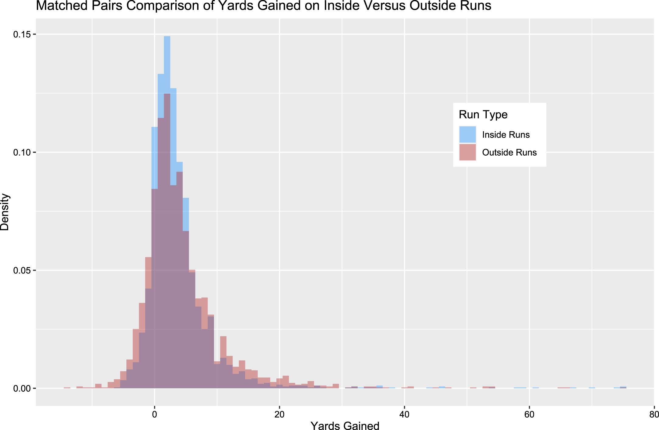
We will attempt to back this claim via two methods. First, if outside rushes are truly linked to positive results in the running game, we should expect a causal relationship to exist between rushing outside and yards gained on carries. To test this, we conducted a matched pairs observational study, using inside versus outside run as the treatment variable and yards gained as the outcome. We matched plays (Ho et al., 2011) according to several variables, requiring exact matches for offensive team, defensive team, season (2017 or 2018 regular season), and early/late down, and relatively close matches (using Mahalanobis distance) for distance to 1st down, line of scrimmage, and score differential. After matching, we had 2628 pairs of plays. After confirming balance amongst covariates, we calculated the average treatment affect (Rubin, 1974) of running outside on yards gained. We observe an expected difference of 0.503 yards gained (95% confidence interval: (0.160, 0.846)), implying that running outside has a significant causal effect on yards gained. Figure 9 shows the distribution of each play in the matched pairs sample, with the color of the histogram bars indicating inside versus outside runs. It again becomes apparent in this plot that outside runs are associated with high risk behavior, as large losses and gains happen at a much more frequent rate than what is observed for inside runs. But it also becomes clear how outside runs would generate more yards on average, with a much larger proportion of big gains occurring, bringing the overall average up.

Fig. 9

Overlapping histograms of yards gained on run plays, with blue bars indicating inside runs and red bars indicating outside runs. Plays are matched using one-to-one nearest neighbor matching based on Mahalanobis distance, with exact matching enforced on some factors.

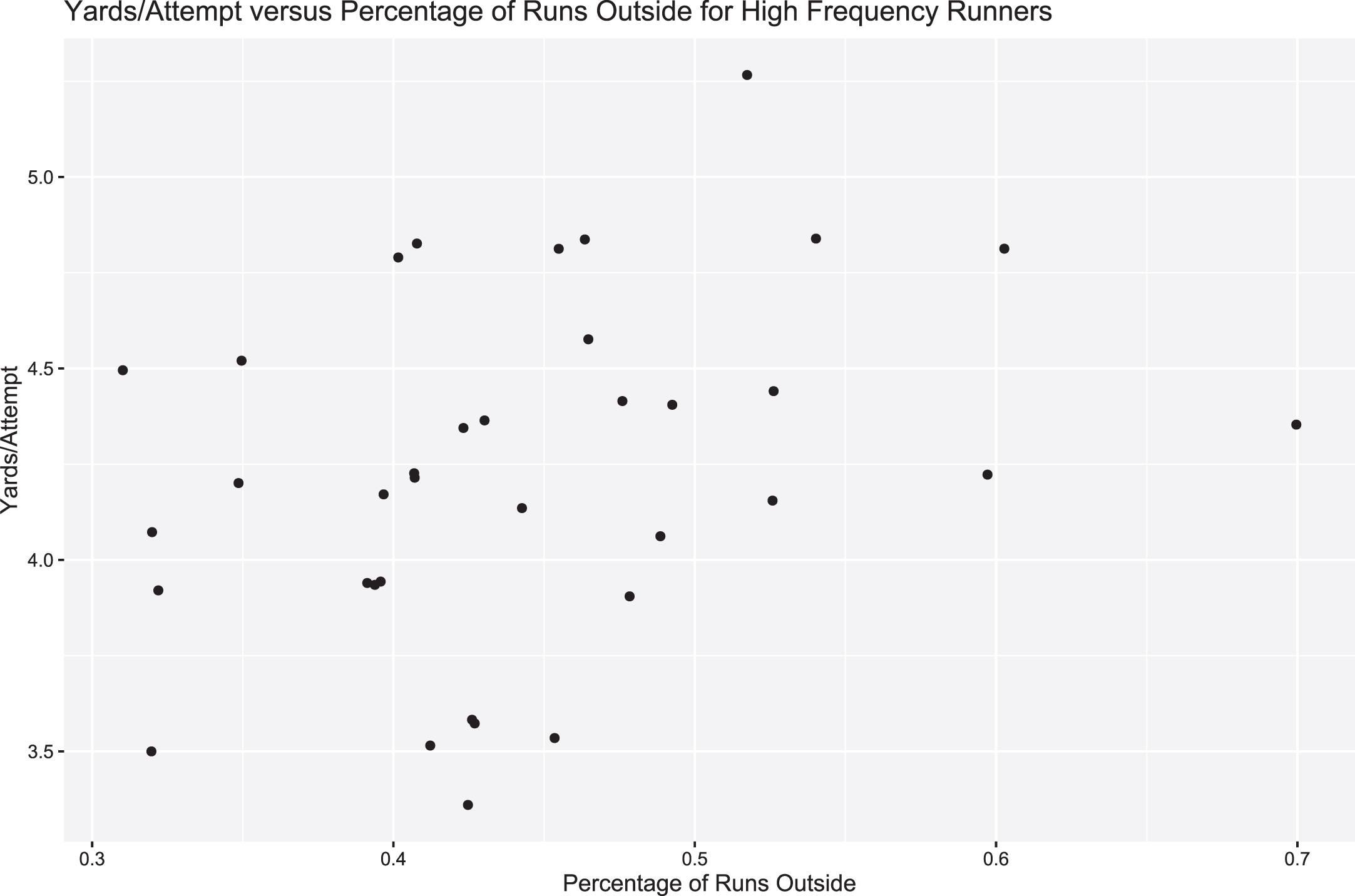
Furthermore, we would expect the same trend to exist at the individual level. Figure 10 shows the relationship between yards gained and percentage of outside runs. Each point represents a player who was the primary rusher for their team during the sample period, removing one outlier (as determined by a standard Cook’s distance outlier test (Cook, 1977)) and all non-primary runners to avoid players with lower sample sizes from clouding the trend. It becomes clear that the trend exists on the individual level, as seen by the positive correlation (r = 0.40) between the two variables. From this, we conclude that there is evidence to suggest that running outside more will generally lead to a more efficient rushing offense, as measured by yards per attempt.

Fig. 10

Scatterplot of yards per attempt versus percentage of runs to the outside for individual runners, specifically for each team’s primary runner, showing a positive correlation in between the variables of interest.

4.1Comparison with EPA

One might suggest that it would be helpful to compare the run parameters with expected points added (EPA) per attempt, as EPA has a direct relationship with points scored in the game. One could obtain a similar plot to Figure 8 for EPA/attempt and notice similar correlations (r = 0.411, p = 0.0195 for variance, r = 0.418, p = 0.0173 for skewness), as seen in Figure 11. The high risk parameters still are associated with an increase in the success metric. One may even wish to explore the relationship between the βTeamξ parameter, which now seems to have a more meaningful relationship.

Fig. 11

Parameters from team adjusted run model plotted against team EPA/attempt.

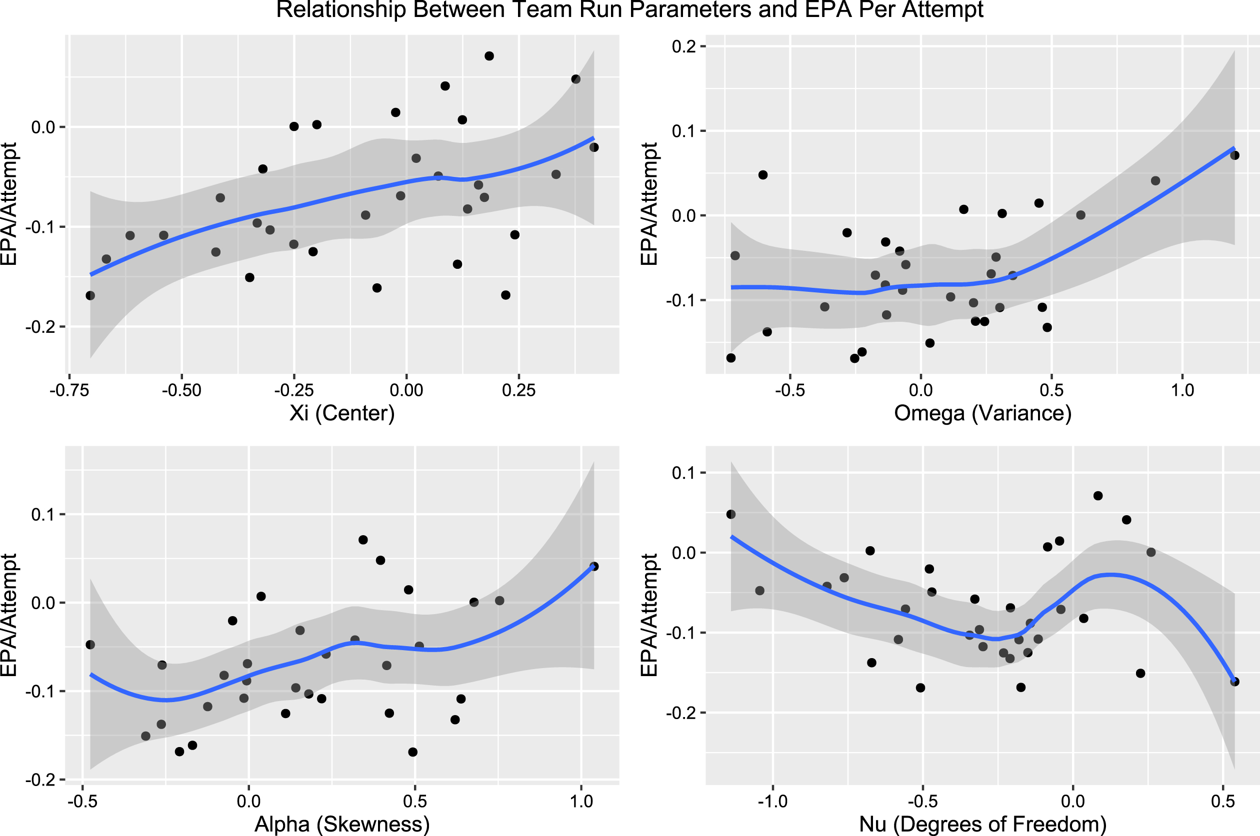
However, an analysis of this type should be done with caution. First, the team adjustment parameters were derived using a model built around yards gained as the output. While correlations likely exist between other metrics related to successful offenses, we should not expect the relationship to necessarily be meaningful or replicable unless the modelling process were adapted to the metric of interest. To do so would require a different density for representation, as EPA does not have the same unimodal, smooth features as seen in the skew-t. Moreover, we find that yards are a better tool for discussion, as EPA is not easy for those with a non-technical background to comprehend, as it can not be directly translated to the game as easily as a physical quantity. When possible, tools such as these should be tailored to the target audience.

5Conclusions

The skew-t mixture model allows for an accurate and efficient calculation of the probability transition distribution for run plays that can be used for the play recommendation system described in Biro and Walker (2022). In addition, the parametric nature created reveals trends that allow us to understand underlying factors related to successful rushing. The variance and skewness shifting parameters led us to finding a preference towards high risk run plays, specifically revealing the benefits of outside running. Exploring this directly led us to finding clear evidence that outside runs are associated with an increased yards per attempt.

The benefits of the parameterized approach are clear, not only providing accurate and consistent distributions, but also allowing for interpretable results. This marries the needs of both the data scientist and the coach, where other models may prove too simplistic to incorporate all necessary features or may be too difficult to be accessible by non-technical audiences.

This work opens up room for several followup projects. The most natural would be the extension of similar parametric models for pass plays. However, the structure of pass plays is dissimilar to run plays, with additional point masses needed for incomplete passes and interceptions, along with a non-unimodal curve that would make a skew-t likelihood unsuitable. Therefore, another parametric approach would be necessary for pass plays.

Furthermore, there are many ways a team could utilize these results in game preparation. This model provides insight into individual team proficiencies and deficiencies in the run game, and therefore can help a team choose which situations are more appropriate for run plays. A team with a larger positive tail in their predictive distribution would generally be better at generating large runs, and therefore running on 2nd and long may be more appropriate than a team with a larger mean but smaller tail, which would be more apt to pick up short yardage situations. Moreover, a team could adversarially influence an opponent to run in situations which they struggle in by properly aligning their defenders. Finally, a team could examine these results thoroughly to determine which run situations they should spend more time practicing.

In addition, there is room for more expansions to the modeling approach here. For example, the model assumes no dependency between plays, and therefore the sequential nature of plays in a football game are lost, as well as the trends that may be captured within a season. For example, over the course of an NFL season, the main runner of a team may become weary or injured, causing the relative success of the team’s running game to decline from week to week. Conversely, at the individual game level, a team may use a run (or pass play) early in the game that tests the defense’s response. How the defense responds could be an indicator to the offensive play caller, and may lead them to use a certain run play for a similar look later in the game that may have more success due to the information revealed in the prior plays. While features like this may be present, it would be difficult to represent them in the current model without well labeled data regarding the nature of the effects in question, which is currently not available. Additionally, adding in dependency effects would reduce the ratio of the number of plays to estimated parameters, implying a lower fidelity in the values obtained.

Finally, adversarial tactics could be considered in future approaches. For example, defensive minds such as Vic Fangio and Brandon Staley have recently been lauded by the analytics community in their ability to invite teams to run the ball in situations typically viewed as detrimental for the offense (Pizzuta, 2021). Thus, using just the offensive team and state information to model run plays (or pass plays) will lack information regarding the defensive structure. However, it still remains necessary to refrain from including post-snap or even at-snap information (such as safety alignment or box counts) in these modeling efforts, as the ability to create prescriptive recommendations would be lost. There are alternatives to these measures, such as using metrics such as defensive trend statistics to inform models, such as expected defensive structure in response to certain offensive alignments. This would require additional data to supplement the current methods such as offensive personnel, formations, and defensive response to each feature, which is not currently publicly available and therefore not explored.

References

1 | Arellano-Valle, R.B. , and Azzalini, A. , (2013) The centredparameterization and related quantities of the skew-t distribution, Journal of Multivariate Analysis 113: , 73–90. |
2 | Baumer, B.S. , and Matthews, G.J. , 2020, teamcolors: Color palettes for pro sports teams, R package version 0.0.4. |
3 | Biro, P. , and Walker, S.G. , (2022) A reinforcement learning basedapproach to play calling in football, Journal of QuantitativeAnalysis in Sports 18: (2), 97–112. |
4 | Burke, B. , 2010a, Expected points and expected points added explained, Advanced Football Analytics, https://web.archive.org/web/20210310003124/http://archive.advancedfootballanalytics.com/2010/01/expected-points-ep-and-expected-points.html |
5 | Burke, B. , 2010b, Win probability added (WPA) explained, Advanced Football Analytics, https://web.archive.org/web/20210310001449/http://archive.advancedfootballanalytics.com/2010/01/winprobability-added-wpa-explained.html. |
6 | Brighenti, C. , 2019, Modelling run outcomes by field control, NFL Big Data Bowl 2020. https://operations.nfl.com/media/4201/bdbbrighenti.pdf |
7 | Carl, S. , and Baldwin, B. , 2022, nflfastR: Functions to efficiently access NFL play by play data, R package version 4.5.1. |
8 | Carroll, B. , Palmer, P. , and Thorn, J. , 1988, The hidden game of football, Warner Books. New York, NY. |
9 | Cook, D. , (1977) Detection of influential observation in linearregression, Technometrics 19: (1), 15–18. |
10 | Coombs, C.H. , and Pruitt, D.G. , (1960) Components of risk in decision making: probability and variance preferences, Journal of Experimental Psychology 60: (5), 265–277. |
11 | Gough, C. , 2022, Development of average offensive yards per game (rushing/passing) in the NFL from 1950 to 2021, Statista https://www.statista.com/statistics/1005862/nfl-average-yards-per-game-developmentover-time/. |
12 | Ho, D. , Imai, K. , King, G. , and Stuart, E. , (2011) MatchIt:nonparametric preprocessing for parametric causal inference, Journal of Statistical Software 42: (8), 1–28. |
13 | Horowitz, M. , Yurko, R. , and Ventura, S. L. , 2017, nflscrapR: Compiling the NFL play-by-play API for easy use in R, R package version 1.4.0. |
14 | Joash Fernandes, C. , Yakubov, R. , Li, Y. , Prasad, A.K. , and Chan, T.C.Y. , (2020) Predicting plays in the National Football League, Journal of Sports Analytics 6: (1), 35–43. |
15 | Lefort, R. , Guo, W. , and Leung, N. , 2022, A machine learning approach to predicting NFL plays, NFLPlayPredictions.com. |
16 | Pearson, K. , (1900) X. On the criterion that a given system ofdeviations from the probable in the case of a correlated system ofvariables is such that it can be reasonably supposed to have arisenfrom random sampling, The London Edinburgh, and DublinPhilosophical Magazine and Journal of Science 50: (302), 157–175. |
17 | Pizzuta, D. , 2021, What NFL defenses need to learn from Brandon Staley & Vic Fangio as two-high looks inevitably rise, Sharp Football Analytics https://www.sharpfootballanalysis.com/analysis/twohigh-shell-staley-fangio-nfl-defense-2021/. |
18 | Ploenzke, M. , 2019, NFL Big Data Bowl sub-contest, NFL Big Data Bowl 2020 https://operations.nfl.com/media/4204/bdbploenzke.pdf. |
19 | Rubin, D.B. , (1974) Estimating causal effects of treatments inrandomized and nonrandomized studies, Journal of EducationalPsychology 66: (5), 688–701. |
20 | Seth, T. , 2020, The NFL’s run gap secret, The Michigan Football Analytics Society https://mfootballanalytics.com/2020/07/15/the-nfls-run-gap-secret/. |
21 | Stern, A. , 2019, Practical applications of space creation for the modern NFL franchise, NFL Big Data Bowl 2020. https://operations.nfl.com/media/4202/bdbstern.pdf. |
22 | Teich, B. , Lutz, R. , and Kassarnig, V. , 2016, NFL play prediction, arXiv preprint, arXiv:1601.00574. |
23 | Winterhalder, B. , (2007) , Oxford handbook of evolutionary psychology: risk and decision-making, Oxford University Press, 433–445. |
24 | Yurko, R. , Ventura, S. , and Horowitz, M. , (2018) nflWAR: Areproducible method for offensive player evaluation in football, Journal of Quantitative Analysis in Sports 15: (3), 163–183. |