
Predictions of european basketball match results with machine learning algorithms
Abstract
The goal of this paper is to build and compare methods for the prediction of the final outcomes of basketball games. In this study, we analyzed data from four different European tournaments: Euroleague, Eurocup, Greek Basket League and Spanish Liga ACB. The data-set consists of information collected from box scores of 5214 games for the period of 2013-2018. The predictions obtained by our implemented methods and models were compared with a “vanilla” model using only the team-name information of each game. In our analysis, we have included new performance indicators constructed by using historical statistics, key performance indicators and measurements from three rating systems (Elo, PageRank, pi-rating). For these three rating systems and every tournament under consideration, we tune the rating system parameters using specific training data-sets. These new game features are improving our predictions efficiently and can be easily obtained in any basketball league. Our predictions were obtained by implementing three different statistics and machine learning algorithms: logistic regression, random forest, and extreme gradient boosting trees. Moreover, we report predictions based on the combination of these algorithms (ensemble learning). We evaluate our predictions using three predictive measures: Brier Score, accuracy and F1-score. In addition, we evaluate the performance of our algorithms with three different prediction scenarios (full-season, mid-season, and play-offs predictive evaluation). For the mid-season and the play-offs scenarios, we further explore whether incorporating additional results from previous seasons in the learning data-set enhances the predictive performance of the implemented models and algorithms. Concerning the results, there is no clear winner between the machine learning algorithms since they provide identical predictions with small differences. However, models with predictors suggested in this paper out-perform the “vanilla” model by 3-5% in terms of accuracy. Another conclusion from our results for the play-offs scenarios is that it is not necessary to embed outcomes from previous seasons in our training data-set. Using data from the current season, most of the time, leads to efficient, accurate parameter learning and well-behaved prediction models. Moreover, the Greek league is the least balanced tournament in terms of competitiveness since all our models achieve high predictive accuracy (78%, on the best-performing model). The second less balanced league is the Spanish one with accuracy reaching 72% while for the two European tournaments the prediction accuracy is considerably lower (about 69%). Finally, we present the most important features by counting the percentage of appearance in every machine learning algorithm for every one of the three analyses. From this analysis, we may conclude that the best predictors are the rating systems (pi-rating, PageRank, and ELO) and the current form performance indicators (e.g., the two most frequent ones are the game score of Hollinger and the floor impact counter).
1Introduction
Basketball is one of the most popular sports in the world. It involves two teams of five players each playing on a court and a maximum of seven substitute players for each team. It is an invasion game whose events are measured in points. During the game, each team aims to throw the ball inside the opponent’s basket. Each successful shot usually accounts for two points (regular throws). Additionally, we may have successful shots from free throws (one point) or long-distance throws (three points). Each game (or match) length is 40 minutes in FIBA competitions (including European competitions) or 48 minutes in the NBA.
A wide variety of data is available during and after each basketball game: shots, assists, rebounds, fouls, steals, turnovers and free throws, among many other statistics. Therefore, basketball is an attractive sport in terms of available data that can be analyzed using statistical models or machine learning algorithms for prediction. The main topic of this article is the prediction of the outcome (in the form of win/loss) of basketball games. We examine the performance of three statistical and machine learning algorithms for basketball prediction using features that have been obtained from team-specific historical data. We focus on data from four major European contests: Euroleague, Eurocup, Greek Basket League, and Spanish Liga ACB. Although a variety of sports studies have been published in several journals, extensive relevant analyses on prediction for European basketball are limited; see for some examples in Horvat et al. (2018), Giasemidis (2020) and Balli & Ozdemir (2021). This work is a systematic attempt to identify which is the best-performed method for basketball outcome prediction in European Basketball.
This paper introduces an enhanced data-set of four European competitions for five seasons in total (2013-2018); a total of 5214 games. Furthermore, we have used new features such as performance indicators (see Appendix 5) and rating systems such as Elo, PageRank and pi-rating (see Section 2.3.2). In addition to the data-set, the paper focuses on answering the following questions: (a) Which method/algorithm performs better in each competition or league? (b) Are the models using box-score statistics, rating systems and performance indicators better than simple vanilla models? And, how much do we gain from the use of additional information? (c) Is the information from previous seasons improving the predictive ability of our models and algorithms? (d) Which features are the most relevant? All models implemented here can be compared with the four-factor model (see Section 4.1.2) and the climatology model (see Section 4.1.3). Finally, the methods and the type analysis implemented for basketball prediction in this paper can be easily adapted for studying their predictive performance in other team sports.
1.1European basketball vs american basketball
Basketball was born in the late years of the 19th century at a college at Springfield, Massachusetts in the USA (see Naismith (1941)). With its genesis taking place in America soon, the sport has migrated across the Atlantic and to many other parts of the world (FIBA was created in 1932). Although basketball nowadays is spread worldwide, there are still basketball fans in the US who are not familiar with European basketball.
American Basketball and more specifically the NBA, which is the top tournament in the USA nowadays, acts independently of the game developments in other countries. The game itself has a variety of differences, both in terms of rules and in terms of the players’ style. One remarkable difference between European basketball and the NBA is the large difference in the average points per game of each player.
In the NBA, many implemented analytics methods have focused on player analysis rather than team analysis (see Gilovich et al. (1985)). Therefore, the performance of a team in the NBA might considerably vary depending on the performance or the availability of the key players. Moreover, a higher number of passes is observed in Euroleague than in NBA games (see Milanović et al. (2014). Finally, there are major differences in the regulations of the game. For example, the three-point line is closer than in the NBA, the defensive 3-second violation is applied in the NBA but not in Europe and the duration of each quarter of the game is 10 minutes versus 12 minutes in the NBA (hence each game is 8 minutes longer in the NBA). These regulations have a huge impact on the game.
1.2Literature review and related work
Basketball is a sport with a variety of game-related events and statistics. The most relevant source of measurement is the box-score, which summarizes the main events of the game and it reflects the performance of the two competing teams. The most prominent works in the field are the publications by Oliver (2004) and Hollinger (2002, 2005). Hollinger (2002) and Oliver (2004) introduced a variety of innovative statistical measures and key performance indicators for the evaluation of the playing quality of each team. Additionally, Oliver and Hollinger provided statistics and projections for NBA players. Another landmark in basketball analytics research is the work of Kubatko et al. (2007) which introduced the basic principles of modern basketball analytics. This work introduced a variety of modern statistical performance indicators and statistics that are widely used in basketball, such as the offensive and defensive ratings, the four factors, the plus/minus statistics, and the Pythagorean method.
In this work, we focus on team performance evaluation and game prediction. One of the first attempts for prediction at basketball games was the work of Schwertman et al. (1991) who focused on models for predicting the probability of each seed winning the regional tournament. Carlin (2005) improved these probability models by using regression models to predict the probability of winning with seed positions, the relative strengths of the teams and the point spreads available at the beginning of the tournament. Smith & Schwertman (1999) concentrated on building more sophisticated regression models for the prediction of the margin of victory using the information provided by seed positions.
Concerning machine learning approaches, the work of Loeffelholz et al. (2009) was one of the first attempts for predicting basketball games. They implemented neural networks, with a variety of performance indicators as inputs, to predict future games in the NBA. As input variables, they used several home and away team statistics, including percentage of shot success, offensive and defensive game statistics averages from previous games and the home effect indicator. Shi et al. (2013) applied three machine learning algorithms (random forest, naive Bayes and multi-layer perceptron) in order to predict NCAA basketball matches for the period 2009–2013. They achieved a prediction accuracy of 74% -75 % using the last approach. Similar is the work of Torres (2013) who, after empirical tuning, used a smaller number of game statistics, taken as an average of the last eight games, in order to predict the final winner for the NBA games of the period 2006-2012. He used four different approaches: linear regression for the final score (and then used the expected difference to predict the winner), a logistic regression model, a support-vector machine and a multi-layer perceptron. He reported a prediction accuracy of 60 - 70% with the best results obtained using the multi-layer perceptron.
Regarding European Basketball, Horvat et al. (2018) predicted Euroleague basketball outcomes using the k-nearest neighbors (k-nn) algorithm. After extensive data manipulation, they implemented the k-nn method for a variety of values of k, selecting the optimal value after a detailed comparison. One of the more recent works on the topic is the publication of Giasemidis (2020) which focuses on the prediction of basketball games in the Euroleague competition using nine machine learning algorithms and statistical models. After this exhaustive implementation of quantitative and machine learning techniques, the main finding was that the opinion of the “well-informed and interested” fans acts better in terms of prediction (66.8% vs 73%). This gives strong rise to the use of modern Bayesian techniques, which can naturally embody both the information coming from data and information for experts and/or other authors.
An additional contribution to this work is the adaptation of popular rating systems from football (soccer). We incorporate in the prediction procedure of basketball outcomes popular rating systems such as the Elo-rating similarly in Hvattum & Arntzen (2010). An alternative rating system we use is the PageRank approach of Lazova & Basnarkov (2015), which ranked the football (soccer), National teams, by considering World Cup results for the period 1930–2015. Finally, we have developed a basketball version of the pi-rating which was introduced by Constantinou & Fenton (2013). Although these rating systems were primarily introduced for rating football (soccer) teams, they can also apply to other sports.
Finally, we also borrow ideas from the inspiring work of Hubáček et al. (2019) where they implemented gradient-boosting for relational data in order to model football (soccer) data. Hence, we predict basketball outcomes of future games within a selected time frame using as predictors specific (a) historical statistics (which reflect the long-term strength of the teams), (b) current form statistics, (c) team ratings, (d) match importance (in the form of dummies for each phase) and (e) leagues statistics.
2Data description and data-set building
The data consists of four different European tournaments from seasons 2013-2018 (five seasons for more details see Table A.2 at Appendix A): (a) Euroleague, (b) Eurocup, (c) Greek Basket League, and (d) Liga ACB. The data-set contains for each team:
• the general game information: the competing teams, in whose stadium each game was performed, the date, the score, and the winner;
• offensive oriented statistics: total number of shots attempted and successful shots for one/two/three points, assists, offensive rebounds;
• defensive oriented statistics: defensive rebounds, blocks, steals, fouls, turnovers.
Fig. 1
Data-set splitting hierarchy according to their usage.
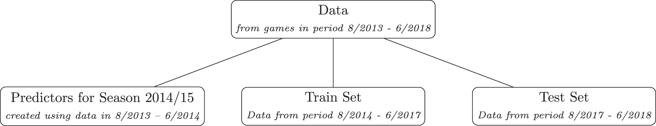
Moreover, for the test data-set, we have examined two additional scenarios: (a) mid-season prediction for the 2017/18 tournament by considering as a training data-set only the results of the first half of the 2017/18 season, and (b) play-off prediction for season 2017/18 by considering in the training data-set all the results of the season 2017/18. Note that all national leagues under consideration do have play-offs phases. For the European tournaments (Euroleague and the Eurocup), as play-offs, we consider the matches in the three final knock-out phases (quarterfinals, semifinals and finals). In addition, for both (a) and (b) prediction scenarios, we have also evaluated and compared the improvement in the prediction metrics when we additionally consider extended learning from the data of all previously available seasons. The main implementation structure of the prediction algorithms (e.g. hyper-parameter tuning, important features, etc.) for all scenarios and leagues has been specified by using the data from the three previous seasons (2014/15–2016/17), namely the hyper-parameter tuning of the machine learning algorithms was accomplished one time per tournament and algorithm. Therefore, the main difference between the scenarios is only the length of the training set and how well the machine learning algorithms learn in these cases. Consequently, the features for every scenario were extracted in the same manner as we describe in Section 2.3.
2.1Main response/target variable
In this paper, the aim is to predict the winner of a basketball game. Hence, the target response variable of interest is the winner of each game. We denote by Yi a binary random variable that indicates the winner of the i game for i = 1, …, n: one when the winner is the home team and zeroes otherwise. Therefore, interest lies in the estimation of the probability that the home team will win, denoted by π and the probability of losing given by q = 1 - π.
2.2Selection of performance indicators and box score statistics
Initially, we generated a wide variety of performance indicators using the box-score statistics of the original raw data-set; see for details in Table B.1 at Appendix B. Using the Pearson correlation coefficient between the score difference of each game and each of these measures, we have proceeded in our analysis by considering only the top-ten correlated performance indicators; see Table C1 at Appendix C. In the following, we will refer to these performance indicators (including the points of each team for the past games) as the “major performance features”.
2.3Features and predictors
Although past information (history) of “major performance features” can give us a good picture of the strength of the two opposing teams in each game, other important characteristics and metrics exist that can also help us predict the final outcome of a basketball game. Such as the current form of a team (that is, performance indicators for a shorter period of recent games) and the overall level of each tournament. Finally, the measures obtained using retrospective rating algorithms can balance the historical and the current form performance of the teams under consideration. So the final selection of features can be separated into four categories:
1. the historical information features: based on results and performance indicators of the games between the two opposing teams and teams’ “major performance features”,
2. the rating systems: team evaluation indicators such as the Elo rating,
3. the current form: teams’ statistics based on the last 10 games,
4. the tournament characteristics features: based on tournament specific statistics and features.
A sample of features can be found in Table E.2 at Appendix E. The main reason for this process is to add more predictors by capturing different aspects of the game. Thus, we can have interpretable information per game, and the machine learning algorithms suggest which of those are can be potentially the important ones per case. As a referee suggested, we should have in mind that when the number of features is large, then some non-important features may be indicated as important by any feature selection method. This might be treated using wrapper feature selection methods (see Kohavi & John (1997)). Here, the number of features is moderate and therefore we believe that this side effect will be minimal. Therefore, we did not pursue this issue further.
In order to implement the proposed procedure, we needed to make some compromises by accepting specific assumptions. As a result, the method has some disadvantages and limitations that should be discussed. First, the teams’ roster frequently changes significantly from one season to another season. Many of the predictors we consider in this work depend on the information from the previous season. However, as the season progresses, all features are updated with more recent and relevant information, adjusting to a more realistic picture of the current season. This problem is more evident in the case that a new team enters the tournament. In this case, we do not have any historical information on the data-set for this team. To resolve the problem, we proceed with a naive solution by using the value of zero for all features of this team for the first game of the season. As the season progresses, the problem diminishes and the features are updated with the relevant information. We believe that this approach has a minor effect on the implemented approach, since the problem is only for a very small number in the data-set (Euroleague: 2.16%, Eurocup: 6.6%, Greek League: 1.82%, Liga ACB: 0.32%) and only for the first game of each season.
In the following sections, we provide details about these four categories of features used in our predictive models and algorithms per tournament.
2.3.1Historical information based predictors
In order to reflect the long-term strength of each team, we have extracted information from all available previous games for a series of variables/features. Using the data from the games between the two opponent teams, we have considered the percentage of wins, point difference and Ediff (the difference between the offensive rating, Ortg, and the defensive rating, Drtg). For these three features, we have extracted three versions of them:
• previous game (based only on previous match-up),
• home previous games (based only on games on the specific home field),
• overall tradition (based on all available games between the two opponents).
Moreover, we have included as possible predictors the means and the standard deviations for all (ten) selected performance features as described in Section 2.2. For all features, we consider two measurements: the achieved and the conceded measurements by the two opponent teams of each game for the previous year (last 365 days); for more details see Table E.1. For the offensive and defensive ratings (Ortg and Drtg) and the Ediff, only one measurement was considered for each of them as defined in Table B.1 and Section 2.2. Finally, 46 additional potential predictors have been considered by taking the differences between the measurements of the home and away teams (see Table E.1).
2.3.2Rating systems
In this category of predictors, we consider three measures based on the rating systems, namely the ELO, PageRank and Pi-rating (for details see Appendix D). Furthermore, the Elo rating system (Appendix D.1) and Pi-rating system (Appendix D.2) have extra tuning parameters that we have to specify in order to optimize them in terms of their selected error measure for these specific basketball tournaments. This adaptation is necessary for their implementation in basketball since these rating systems were initially tuned for football (soccer).
For the Elo rating system, we tune the parameters after considering values of k0 = 1, 2, 3, …, 60 and λ = 0.1, 0.2, 0.3, …, 3.5 (see Appendix D.1). We tune the parameters by minimizing the mean absolute difference between the probability of the home team winning and the actual game outcome for the accumulated data of seasons 2013/2014 - 2016/2017 for each tournament (Euroleague, Eurocup, Greek League, Liga ACB). Figure 2 depicts the minimization values for each tournament while Table 1 summarizes the tuned values for each tournament. In the last row of Table 1, you can find the means of the optimal k0 and λ across the four tournaments. These values can serve as default “good” values when the ELO rating is applied to other basketball tournaments. The same procedure is followed for Pi-rating, see Appendix D.3, Table D.3.1 and Figure D.3.1. From these measurements, we calculate the value of each rating for each opponent team in a game, and then we consider their differences; see Table E.1c for a summary of the predictors used in this category.
Fig. 2
Plot for finding the optimal mean absolute difference for a grid of k0 and λ Elo parameter values.
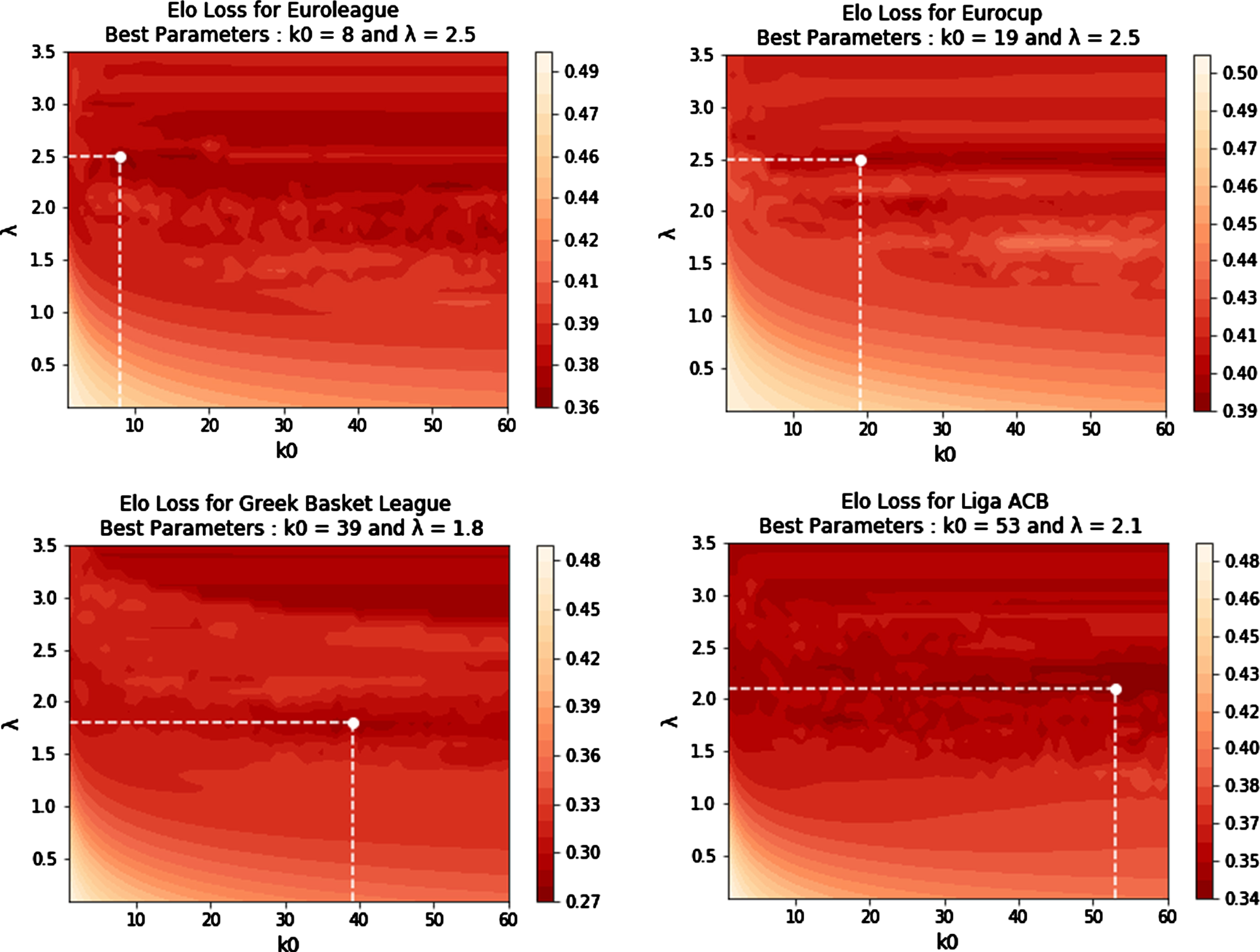
Table 1
Summary statistics of the tuned Elo parameters
| Tournament/ League | k0 | λ | Minimum mean absolute difference | Mean absolute difference of average parameters | Differences of mean absolute differences |
| Euroleague | 8.00 | 2.50 | 0.36 | 0.37 | 0.01 |
| Eurocup | 19.00 | 2.50 | 0.39 | 0.42 | 0.03 |
| Greek League | 39.00 | 1.80 | 0.28 | 0.31 | 0.03 |
| Liga ACB | 53.00 | 2.10 | 0.34 | 0.34 | 0.01 |
| All leagues (Average) | 29.75 | 2.25 | 0.34 | 0.36 | 0.02 |
A standard practice is to use these rating systems as standalone predictions (see Hvattum & Arntzen (2010), Lazova & Basnarkov (2015),Constantinou & Fenton (2013)). An evaluation of the predictive performance of these rating systems is presented in Appendix H.1. For each rating, we calculated the rating value of each team before the match of interest and we predicted the winner according to the higher rating/rank of the two opponents. In table H.1.1, we present the predicted accuracy of these simplistic rating system-based approaches for the season 2017-2018. The results are quite competitive compared to simple statistical models or machine learning algorithms; see Section 4.1.1 for more details. Moreover, as we will see in the following (see Section 4.6) all rating systems are extremely good predictors/explanatory variables when they are used as input features in the machine learning algorithms under study.
2.3.3Current team form
The performance of athletes and/or teams fluctuates during a season with a period of higher or lower performance, which can depend on several characteristics such as psychology, practice program, stamina or the level of difficulty of games played. This is commonly known by the fans as the “current form” of the team and it refers to the performance of the team or athlete over the recent past (say the last ten games). The category of features described in this subsection is used in our predictive models and algorithms in order to record the current form of the European Basketball teams we study. To do so, we have included all features of Table E.1b and the ratings of Table E.1c but calculated only for the last ten matches.
By using as features a mix of historical summary information (within one year time span) and current form information (within 10 games time span), we consider both the long and the short term effect of box-score statistics and rating systems on the final match outcome. As a referee proposed, a more appropriate approach would have been to consider a weighting scheme that gives more importance to the latest matches that naturally better reflects the current performance of a team. Ideally, such weights should have been estimated from our data-set.
This is an interesting research direction that the authors are intrigued to pursue in the near future but, we believe, outside the scope of this article where we identify the effect of specific features and models.
2.3.4Tournament specific statistics and characteristics
Following Hubáček et al. (2019), the fourth group of features we consider in our predictive analysis consists of tournament-specific characteristics. In this way, we try to account for and adjust our predictions for the difficulty of each league or competition. Hence, we consider all measures of Table E.1b over the last year (365 days) for each tournament. Note, that unlike Hubáček et al. (2019) where the corresponding league-specific features were constant within each tournament, here the tournament features are dynamically updated after every game-day. Three features (percentage of wins, point difference and Ediff) have been calculated from the perspective of the home team while, for the remaining ones, we have considered the difference between home and away teams. Finally, we have further included a tournament phase indicator since the phase of each tournament (regular season, play-offs, final four, etc.) can determine the performance and the motivation of each team. This variable was included by using a set of dummy indicator variables.
2.3.5Final Details: Feature dimension and transformation
A total of 110 features are finally used in this study. Therefore, we cover a wide variety of features of interest that, hopefully, capture all possible aspects of the game. The aim of considering such a large number of covariates is to act in an exploratory fashion and discover or reveal hidden patterns in the game of basketball. Hence, in our analysis, we leave each machine learning algorithm to suggest which are the important features via the implementation of the appropriate variable selection method for each algorithm. As one referee pointed out, the large number of features may be a problem due to the multiple comparisons we consider (multiplicity problem) resulting in false positive features. Nevertheless, we have considered different analyses and different methods and we report in how many of these cases each variable was found to be important. This hopefully avoids systematic false positives. Hence, a feature that is not a true explanatory variable for the match outcome may appear in a limited number of cases as important but its overall reported percentage will be low.
Due to differences in the scaling and distributions of features, we have transformed all arithmetic features in order to lie in the [0,1] interval. The transformation is implemented within each tournament separately. To do this, we have used the min-max normalization which is given by:
(1)
Another alternative would have been to use z-scores given by
3Classification models and algorithms
Due to the large number of predictors we consider in this work, we focus on the implementation of methods where a variable selection or screening methods could be implemented in an automatic way. In this wise, we have better predictions and we can emphasize in the interpretation. For this reason, we have implemented three major interpretable predictive approaches:
1. Logistic Regression with Regularization (see Appendix F.1)
2. Random Forest (see Appendix F.2)
3. Extreme Gradient Boosting (see Appendix F.3)
All methods were implemented using scikit-learn and XGBoost python libraries. The tuning parameters and the variable selection or screening procedures for every classification algorithm have been implemented using randomized search with 10-fold cross-validation (CV) in the training set for every tournament separately (see in Section 2). We tune our models in the 10-fold CV by using Brier score (BS) (see Appendix G.1). In the following, besides the Brier score (BS), we use the accuracy (see Appendix G.2) and the F1 scores (see Appendix G.3) for checking the final predictive ability of the implemented methods.
3.1Ensemble learning
Ensemble learning methods are essentially model averaging techniques that consider the mean of predictions of different predictive models and/or algorithms. The intuitive idea of combining different models’ predictions is that each model can capture different aspects of the game or correct for a poor assumption made by a model; see Cai et al. (2019) for implementation of basketball data. The Random Forest and the XGBoost techniques, for example, are ensemble types of algorithms that combine predictions from many trees. Nonetheless, the two algorithms are completely different in logic, usually leading to different predictions. Hence, the idea here is to combine all three different algorithms implemented in this work (logistic regression, random Forrest and XGBoost) by taking the average of the predicted probabilities. This will hopefully lead to more robust and reliable predictions.
4Empirical results
In our main analysis (referred to in the following as full season analysis), the first season (2013/14) is used to build our initial predictors of the predictive models for season 2014/15. The three sequence seasons (2014/15, 2015/16, 2016/17) are used as our training data-set, while the last one (2017/18) is used as a test/validation data-set.
We have further considered two predictive analyses which are of interest from the basketball fan or bettor’s perspective:
(a) Mid-season predictive analysis using the features of the first half of the regular season 2017/18 for training, in order to predict the outcome of the games of the second-half,
(b) Play-offs predictive analysis using all features of the regular season 2017/18 for training in order to predict the play-offs final results for season 2017/18.
4.1Benchmark models
4.1.1Baseline vanilla models as starting reference analysis
A standard approach in data science and machine learning is to consider a simple “vanilla” or “benchmark” model as a starting point in our analysis (see Stefani (1980)). Such models are constructed using only the minimum pre-game information available as predictors. Hence, the predictors are only based on the team names (or labels) playing in each game and which team is the host (playing at its home stadium). The standard approach is to consider a constant home effect for all competing teams. The assumption of the constant home effect has been validated and tested on several occasions in basketball (Harville & Smith (1994)).
We have fitted our Baseline Vanilla Model to the three different prediction scenarios under consideration (full season, mid-season and play-offs). For the logistic regression, we have considered a regularized version of the model, which implies that a reference group of teams of similar strength is formed automatically by the imposed methodology. In order to implement the Baseline Vanilla Model, we have specified one feature/covariate for each team. These features are coded in the following form of dummy variables:
(2)
We will refer to this model as the “Baseline Vanilla Model”. The exponent of the intercept of the vanilla logistic regression model can be interpreted as the common home effect of the teams in the tournament; see Table H.4.1 for the estimated intercept parameters for the four tournaments under study under the full season prediction scenario. Specifically, the intercept is equal to the log-odds of the win for the home team when two teams of equal strength compete with each other.
4.1.2Oliver’s four factor model
A benchmark logistic regression model was created with Oliver’s four factors as covariates (see Oliver (2004)), namely: (a) the effective field goal percentage, (b) the offensive rebounding percentage, (c) free throw rate and (d) turnover percentage. These factors were reported by Oliver (2004) as predictors highly correlated with the final game result in basketball. In this implementation, Oliver’s factors are calculated as the average of the last 10 matches of each team. The results of this benchmark model are presented in Appendix H.2.
4.1.3Climatology model
Finally, a simple climatology model (see Brier et al. (1950), Murphy (1973)) was also used as a reference, after the suggestion of a referee. This model is essentially a model which assumes a constant probability of success for the home (and away) team, see Giasemidis (2020 (“the home team always win”). In our case, we have used as baseline win probability for the home team values in the interval of 55-65%. The brier skill scores from this simple approach are provided in Appendix H.3.
4.2Predictive evaluation of the full season 2017/18
For the full data-set of season 2017-2018, all final models are compared with
(a) the Baseline Vanilla Model introduced in Section 4.1.1
(b) the Full Information Model (i.e. predictive models with features of Table E.1) introduced in Section 2.3.
From Tables 2 and 3, it is evident that the Full Information Model performs better in terms of Brier score, accuracy and F1-score for all tournaments; see Figure 3 for a graphical representation of the differences between the two models. The lowest differences between the predictive scores of the two models are observed in Euroleague. Especially, the Brier score difference is very close to zero, indicating that the extra included does not considerably improve the predictive performance of the model. This might be because the Euroleague is the most balanced and unpredictable tournament, since all participating teams are top-class European teams. On the contrary, the Full Information Model presents its highest predictive improvement in comparison to the Baseline Vanilla Model in Eurocup, where the results are more predictable. The Eurocup is more unbalanced in terms of competitiveness of the participating teams than the Euroleague, characterized by a small group of strong teams and another group of teams that are not interested in this tournament. Teams of the latter group do not perform in a reliable way, making the corresponding predictions difficult when game-specific information is not included in our predictive model. Hence, the Full Information Model seems to capture these differences efficiently in Eurocup via the extra information introduced by the additional features taken into consideration.
Table 2
Summary prediction measures for the Baseline Vanilla Model in the full season prediction scenario; see Table H.4.2a for more details
| Tournament/ | Brier Score | Accuracy | F1 | |||
| League | Interval | Best Model(s) | Interval | Best Model(s) | Interval | Best Model(s) |
| Euroleague | 0.213–0.215 | RF/EL | 0.650–0.665 | RF | 0.745–0.767 | RF |
| Eurocup | 0.232–0.238 | LG/EL | 0.625–0.636 | LG/RF | 0.717–0.729 | RF |
| Greek League | 0.167–0.181 | LR | 0.735–0.745 | RF/EL | 0.804–0.814 | RF/EL |
| Liga ACB | 0.208–0.218 | LR/RF | 0.648–0.688 | RF | 0.733–0.767 | RF |
LR: Logistic Regression; RF: Random Forrest; XGB: Extreme gradient boosting; EL: Ensemble learning; Interval: Min - Max evaluation score of ML algorithms
Table 3
Summary prediction measures for the Full Information Model in the full season prediction scenario; see Table I.1a for more details
| Tournament/ | Brier Score | Accuracy | F1 | |||
| League | Interval | Best Model(s) | Interval | Best Model(s) | Interval | Best Model(s) |
| Euroleague | 0.208–0.220 | XGB | 0.662–0.692 | XGB | 0.749–0.778 | XGB |
| Eurocup | 0.205–0.216 | RF | 0.641–0.690 | XGB | 0.748–0.761 | RF |
| Greek League | 0.145–0.150 | LR/EL | 0.755–0.784 | EL | 0.818–0.839 | EL |
| Liga ACB | 0.197–0.201 | EL | 0.697–0.719 | EL | 0.783–0.788 | EL |
LR: Logistic Regression; RF: Random Forrest; XGB: Extreme gradient boosting; EL: Ensemble learning; Interval: Min - Max evaluation score of ML algorithms
Fig. 3
Comparison of the differences of evaluation metrics between the best performed methods of the Full Information and the Baseline Vanilla Model for the full season prediction scenario.
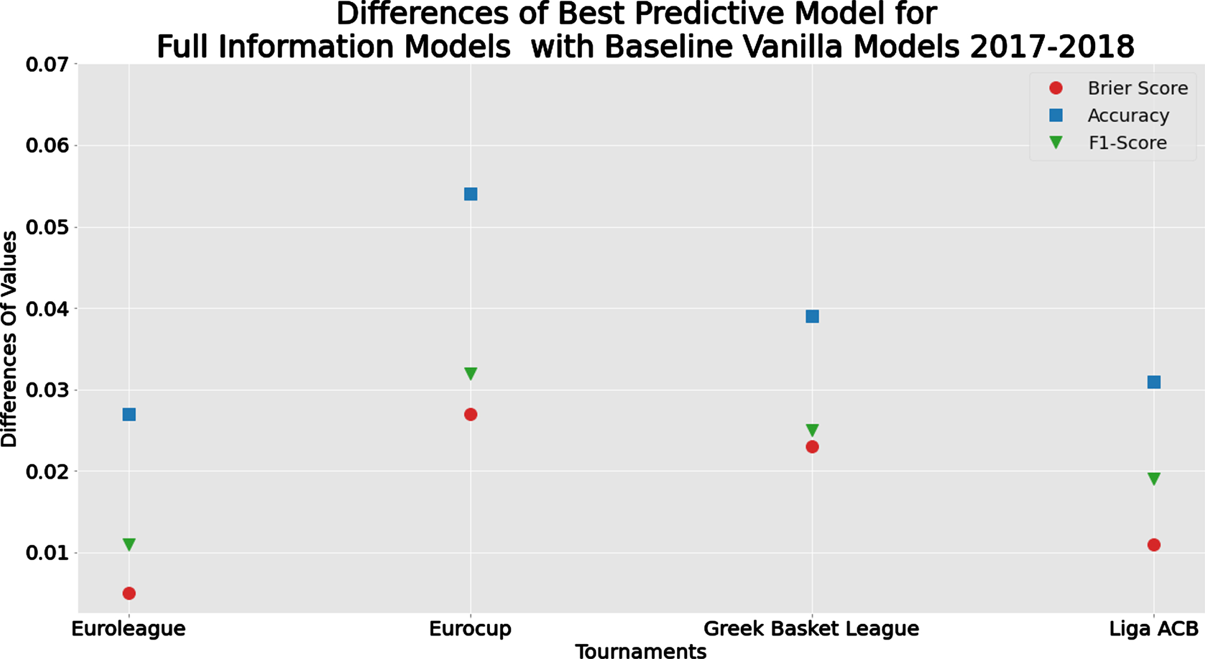
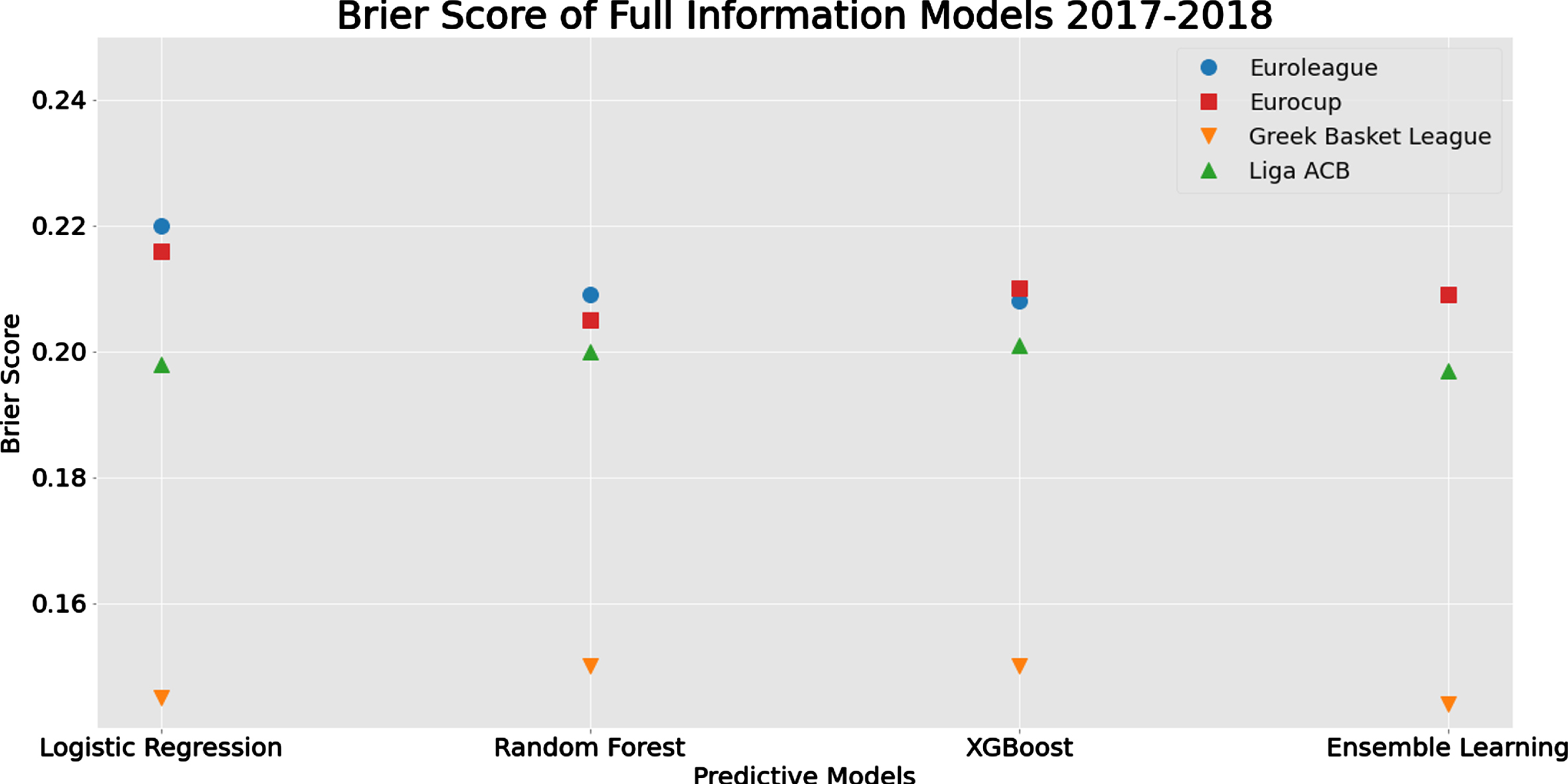
Figure 4 presents the Brier score for the Full Information modeling approach for all classification models under consideration for each tournament (presented on each line). From this figure, it is obvious that the Greek league is the most predictable of the four tournaments under consideration with all models achieving similar Brier scores. On the other hand, both Euroleague and Eurocup seem to be less predictable with similar levels of predictive performance (Brier score ∼ 0.205 - 0.22). The logistic regression was found to systematically perform slightly worse than the other two methods. Finally, the Spanish Liga ACB is also close to the European tournaments but slightly more predictable (Brier score 0.197-0.201). All three classification models are identical in terms of predictive performance, as in the Greek league. Similar are the conclusions (with more variability in the values) for the accuracy and the F1-score; see Figure J.1 at Appendix J.
Fig. 4
Comparison of methods and algorithms in terms of Brier Score for Full Information Models for each tournament for the full season prediction scenario.
For the other two benchmark models (Oliver’s four factor model and the climatology model), we observe that the Full Information Model is systematically better (as expected). To be more specific, from Table H.2.1 we observe that the accuracy for the four leagues ranges from 0.62 to 0.75, which is systematically lower than the corresponding values for the Baseline Vanilla Model (0.63–0.735) and the full information model (0.64-0.77; differences 0.02–0.052). The only case where the four factor model is better in terms of accuracy than the Baseline Vanilla Model is the Greek league with accuracy values of 0.75 vs. 0.735, respectively. For the other three competitions, the accuracy differences are 0.016, 0.023 and 0.037 in favor of the Baseline Vanilla Model (in ascending order). Finally, for the climatology model, the percentage improvement induced by the use of the Full Information Model instead of the climatology one ranges, in terms of Brier score, from 5% to 40% depending on the tournament, the method used and the assumed probability of winning for the home team.
4.3Mid-season predictive evaluation
In this section, we focus on the prediction for the second half of season 2017/18. This approach tries to follow the interest of the basketball fans and bettors for specific landmarks of the season. The prediction in the middle of the regular season is commonly used in related bibliography (see for example Heit et al. (1994)) since the accumulated information is enough to learn/estimate the model parameters and obtain reliable predictions. Here, we use the structure and the values of the hyper-parameters obtained by the analysis of seasons 2014–17 (three seasons in total) as described at the beginning of Section 4. Then, given the model structure and the hyper-parameter values, the data of the first half of Season 2017/18 were used for learning about the parameters of each classification model. By using this approach, intuitively some effects may be estimated more reliably from the data of the current season rather than from previous seasons where the roster and team performance was different (see Zimmermann (2016).
We expect this to be true in the vanilla modeling approach. Nevertheless, for the Full Information Model, learning from all previous data (i.e. of seasons 2014–17 and the first half of 2017/18) might be more effective in terms of prediction since the covariate/feature information (which indirectly reflects the performance and the quality of the roster of a team) is adopting from season to season (e.g. the feature measuring each team performance in the last ten games).
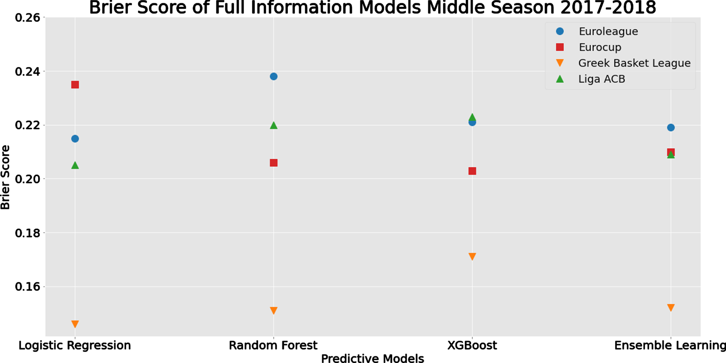
Summary of the predictive performance measures for the Baseline and the Full Information Models is given in Tables 4 and 5, respectively. Concerning the differences between the best models (see Figure 5), the predictive performance is similar to the full season analysis (Section 4.2) where we observe that the Full Information Model is identical to the Baseline Vanilla Model (differences are very close to zero) for Euroleague. On the contrary, for the Eurocup, we observe the highest differences for the reasons discussed in Section 4.2. From Figure 6, we observe again that the Greek league is the most predictable tournament while the other three tournaments are quite close in terms of Brier score. A difference with the results of Section 4.2 is that the logistic regression model here seems to outperform its competitors for all tournaments except for the Eurocup. This is mainly due to the simpler structure of the logistic regression model in comparison with the other predictive models which require larger datasets in order to learn efficiently and provide reliable predictions.
Table 4
Summary prediction measures for the Baseline Vanilla Model in the mid-season prediction scenario; see Table H.4.2.b for more details
| Tournament/ | Brier Score | Accuracy | F1 | |||
| League | Interval | Best Model(s) | Interval | Best Model(s) | Interval | Best Model(s) |
| Euroleague | 0.204–0.214 | XGB | 0.650–0.692 | XGB | 0.753–0.776 | XGB |
| Eurocup | 0.216–0.245 | LR | 0.560-0.667 | RF | 0.718–0.754 | RF |
| Greek League | 0.171–0.189 | RF | 0.703–0.747 | EL | 0.809–0.827 | EL |
| Liga ACB | 0.210–0.220 | EL | 0.634–0.686 | EL | 0.723–0.774 | EL |
LR: Logistic Regression; RF: Random Forrest; XGB: Extreme gradient boosting; EL: Ensemble learning; Interval: Min - Max evaluation score of ML algorithms
Table 5
Summary prediction measures for the Full Information Model in the mid-season prediction scenario; see Table I.1b for more details
| Tournament/ | Brier Score | Accuracy | F1 | |||
| League | Interval | Best Model(s) | Interval | Best Model(s) | Interval | Best Model(s) |
| Euroleague | 0.215–0.221 | LR | 0.600–0.692 | EL | 0.733–0.804 | EL |
| Eurocup | 0.203–0.235 | XGB | 0.571–0.726 | RF | 0.723–0.793 | RF |
| Greek League | 0.146–0.171 | LR | 0.747–0.78 | LR/EL | 0.813–0.841 | LR/EL |
| Liga ACB | 0.205–0.223 | LR | 0.614–0.712 | LR | 0.751–0.798 | LR |
LR: Logistic Regression; RF: Random Forrest; XGB: Extreme gradient boosting; EL: Ensemble learning; Interval: Min - Max evaluation score of ML algorithms
Fig. 5
Comparison of the Differences in Evaluation Metrics between the best performed methods of the Full Information and the Baseline Vanilla Model for the mid-season prediction scenario.
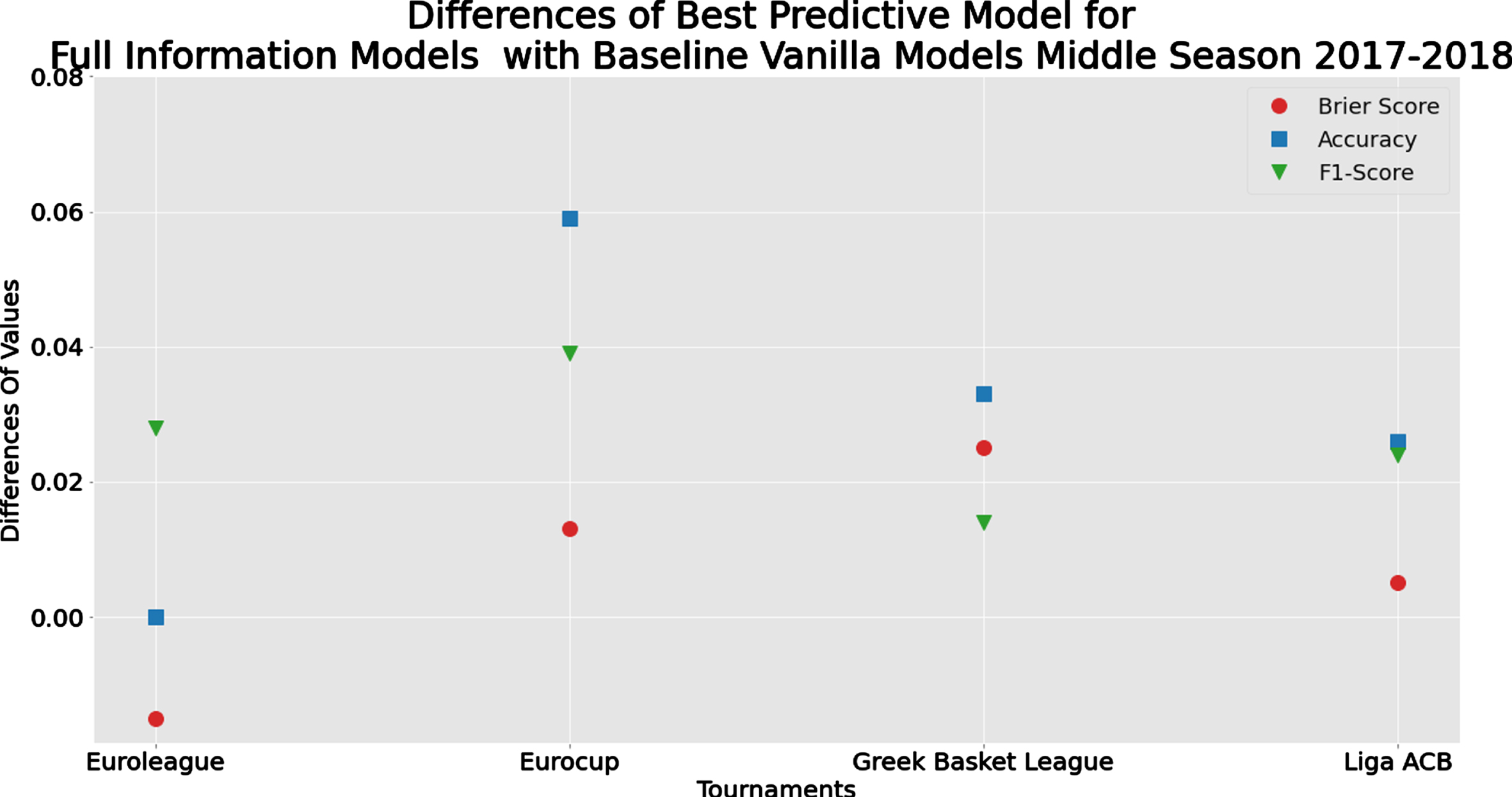
Fig. 6
Comparison of methods and algorithms in terms of Brier Score for Full Information Models for each tournament for the mid-season prediction scenario.
4.4Play-offs predictive evaluation
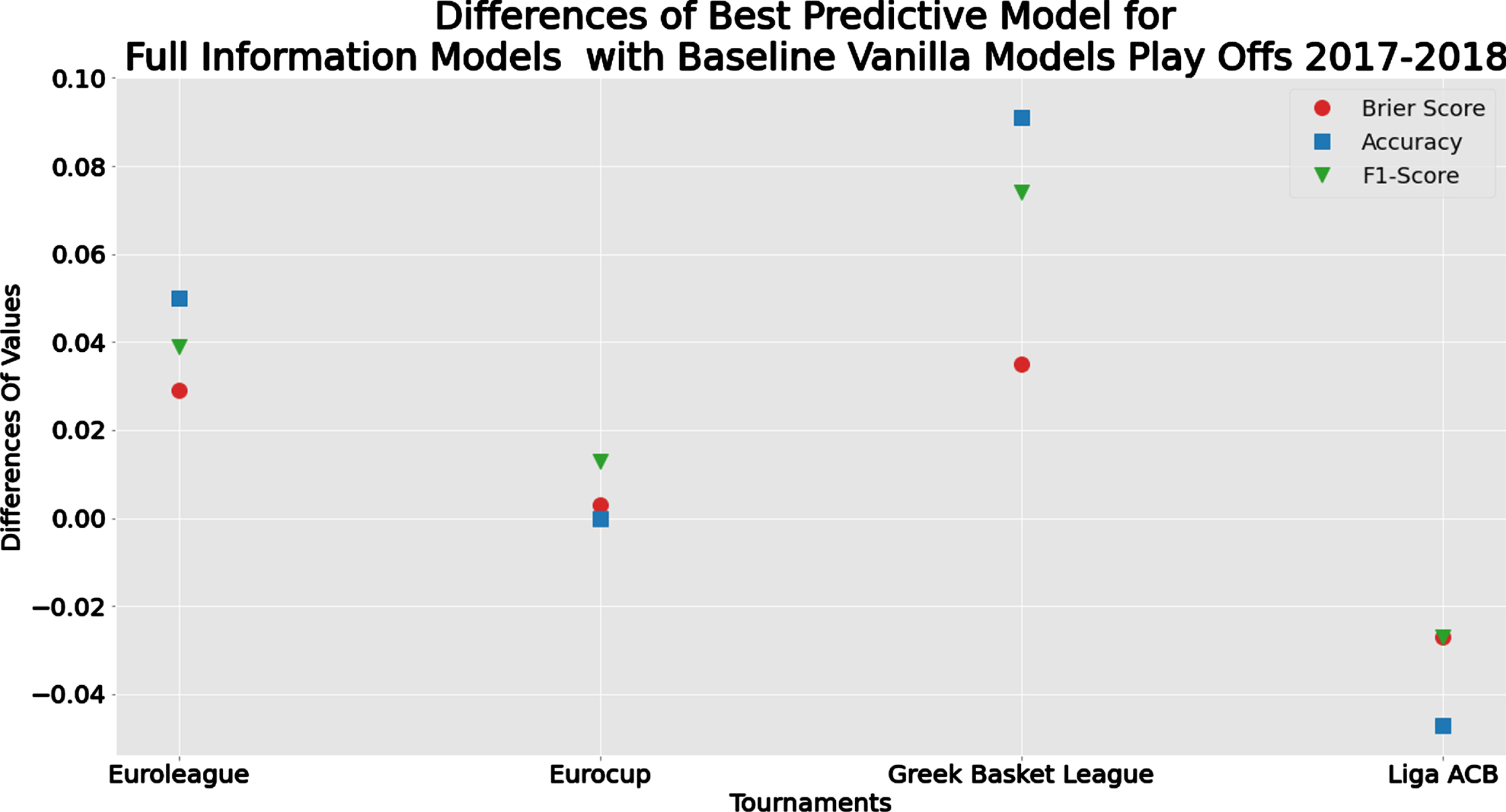
The second season landmark we use for prediction is the end of the regular season where we wish to predict the results of the play-offs game which are the highlight of the whole season. Hence, we implement a similar procedure as in Section 4.3 but now the test set is comprised only of the games of the play-offs for season 2017/18. For the Euroleague and the Eurocup, we consider as play-offs the quarterfinals and the games of the subsequent phases. In this analysis, a point of caution is the fact that the size of the test set is small. Therefore, the variability of the prediction evaluation metrics can be high or considerably influenced by the inefficient performance of a specific algorithm in one game. A surprising result in this analysis is the fact that the baseline model outperforms the Full Information Model for the Liga ACB play-offs. Notably, the accuracy in Liga ACB for the random forest full information implementation was found to be only slightly better than the pure chance (53%). This is partly due to the fact that our models have been trained with regular season results, which can be different from play-offs, since it includes games that are of no interest for particularly strong teams. For the rest of the tournaments, the Full Information Model outperforms the baseline as expected.
Summary of the predictive performance measures in the play-offs for the Baseline and the Full Information Models are given in Tables 6 and 7, respectively. Concerning the differences in the predictive measures between the best models (see Figure 7), the results are different from the ones obtained in the full and mid-season analyses (Sections 4.2 and 4.3) since now we observe that the Baseline model is slightly better, in terms of predictive performance than the Full Information Model, for the Liga ACB (as noted before) and the two models are identical for Eurocup. For the other two tournaments (the Greek league and Euroleague), the Full Information Model achieves better predictive performance in the play-offs as previously in the full and mid-season analysis.
Table 6
Summary prediction measures for the Baseline Vanilla Model in the play-offs prediction scenario; see Table H.4.2c for more details
| Tournament/ | Brier Score | Accuracy | F1 | |||
| League | Interval | Best Model(s) | Interval | Best Model(s) | Interval | Best Model(s) |
| Euroleague | 0.221–0.283 | LR | 0.600–0.700 | LR | 0.692–0.800 | LR |
| Eurocup | 0.168–0.213 | RF | 0.688–0.750 | RF/EL | 0.762–0.833 | RF |
| Greek League | 0.160–0.202 | LR | 0.636–0.773 | EL | 0.750–0.815 | EL |
| Liga ACB | 0.190–0.221 | EL | 0.714 | ALL | ||
LR: Logistic Regression; RF: Random Forrest; XGB: Extreme gradient boosting; EL: Ensemble learning; Interval: Min - Max evaluation score of ML algorithms
Table 7
Summary prediction measures for the Full Information Model in the play-offs prediction scenario; see Table I.1c for more details
| Tournament/ | Brier Score | Accuracy | F1 | |||
| League | Interval | Best Model(s) | Interval | Best Model(s) | Interval | Best Model(s) |
| Euroleague | 0.192–0.226 | RF | 0.650–0.750 | XGB/EL | 0.774–0.839 | XGB/EL |
| Eurocup | 0.165–0.191 | RF | 0.688–0.875 | LR/RF/EL | 0.783–0.846 | LR |
| Greek League | 0.125–0.148 | XGB | 0.773–0.864 | XGB | 0.815–0.889 | XGB |
| Liga ACB | 0.217–0.249 | XGB | 0.524–0.667 | XGB | 0.668–0.759 | XGB |
LR: Logistic Regression; RF: Random Forrest; XGB: Extreme gradient boosting; EL: Ensemble learning; Interval: Min - Max evaluation score of ML algorithms
Fig. 7
Comparison of the differences in evaluation metrics between the best performed methods of the Full Information and the Baseline Vanilla Model for the play-offs prediction scenario.
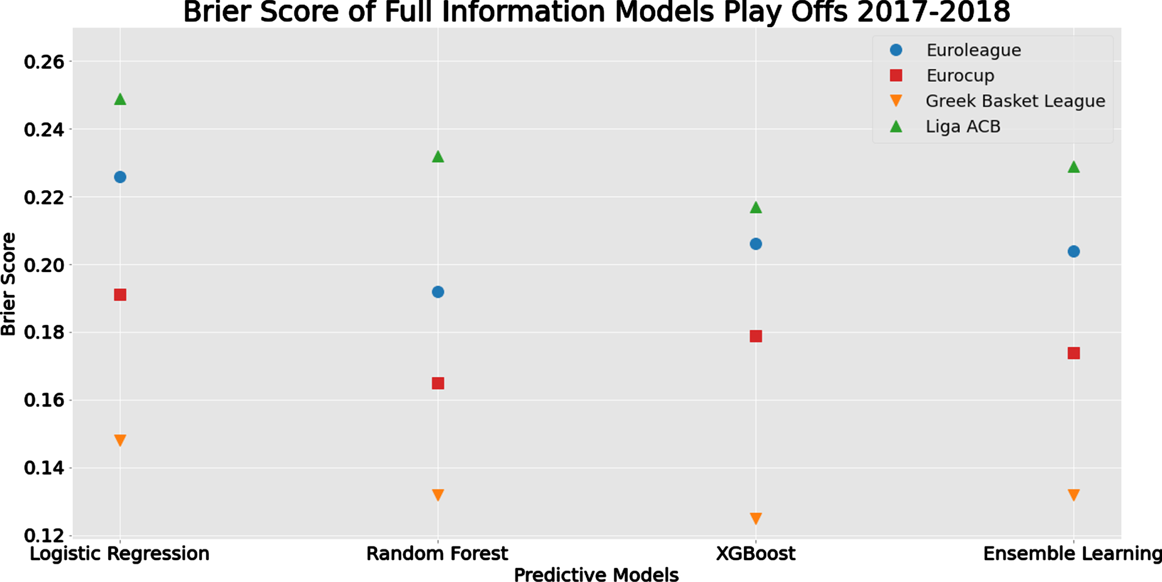
From Figure 8, we observe again that the Greek league is the most predictable tournament in terms of Brier score, while the Liga ACB is the least predictable one with the two European tournaments somewhere in the middle. In terms of classification methods, XGBoost and Random Forest outperformed the other two approaches, with the first one being better for the two national leagues under study (Greek and Spanish), while the latter method was for the European Tournaments.
Fig. 8
Comparison of Brier Score for Full Information Models for each tournament for the play-offs prediction scenario.
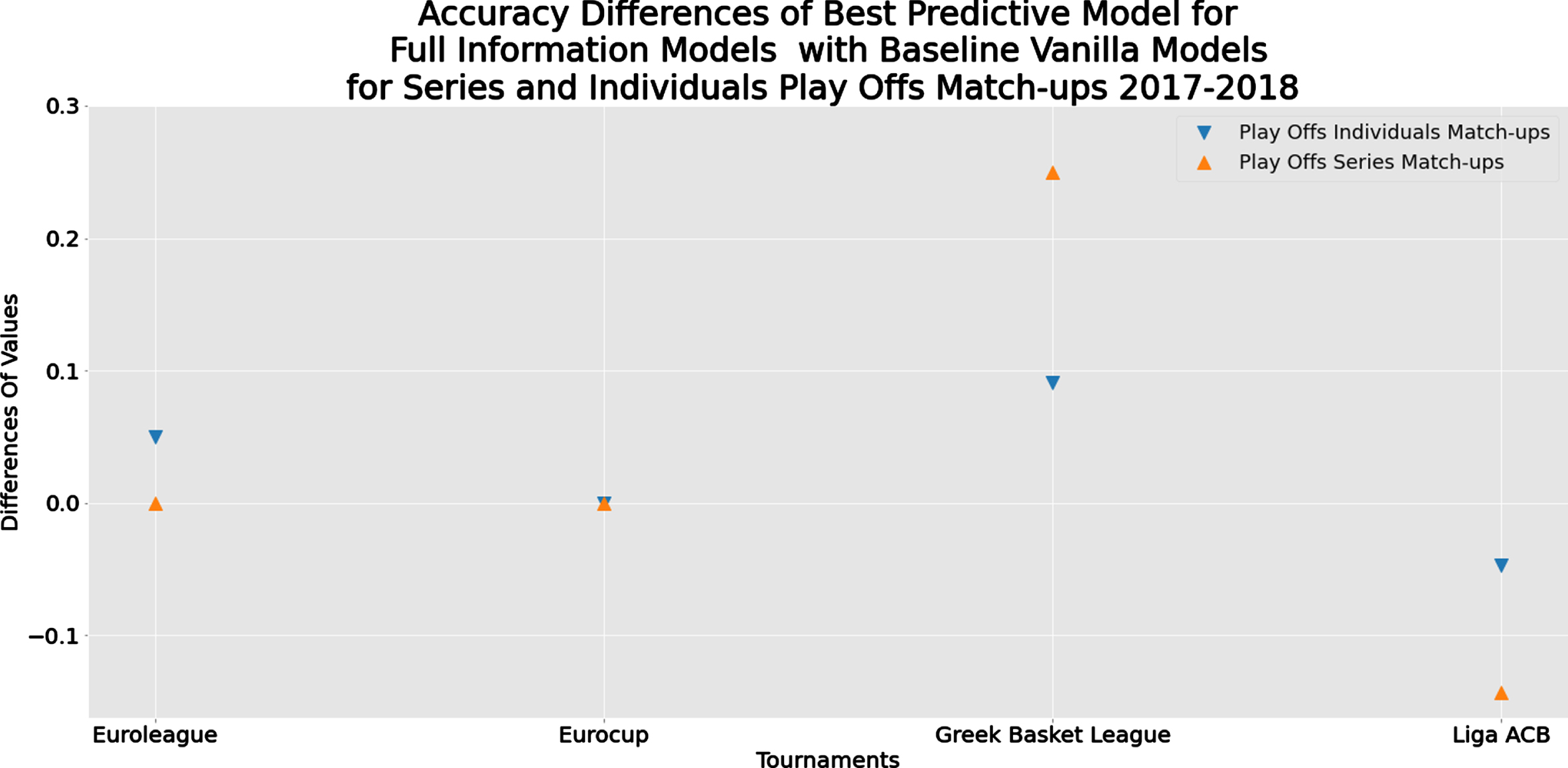
Finally, as the referee suggested, we also present the accuracy measures for the predictions of the series of games in play-offs; see Table K.1 at the appendix K for details. Figure 9 depicts the accuracy differences between the Full Information Model and the Baseline Vanilla Model concerning the individual games and the winner of each play-offs series of games. Generally, the accuracy differences are close for the two cases with no clear patterns.
Fig. 9
Comparison of the accuracy differences of evaluation metrics between the best performed methods of the Full Information and the Baseline Vanilla Model for series and individuals play-offs match-ups 2017-2018.
4.5Comparison training sets for mid-Season and play-offs
The aim of this section is to compare the performance of the predictive models under different learning data-sets for the mid-season and the play-off prediction scenarios for both model versions (Baseline Vanilla Model and Full Information Model). We examine whether using the full history (including features from all previous three seasons additionally to the features from the current season) improves the predictive performance of the fitted models in comparison with the case of using only the features of the current season (i.e. using only the first half-season results or the full season result respectively for the two prediction scenarios).
Figure 10 presents the mean Brier score of all four models using bars. Additionally, the variability of the prediction efficiency across the four methods is represented via error bars. Narrow error bars imply that all classification methods have similar predictive performance as measured by Brier score, while wide error bars indicate differences in the predictive performance. Hence, in the latter case, selecting the best performing model might considerably improve the predictive efficiency.
Fig. 10
Comparison of methods and algorithms in terms of Brier score performance in the mid-season scenario for the Full Information and Baseline Vanilla Models over different tournaments/leagues and different set of training data-sets (current mid-season vs. all previous games).
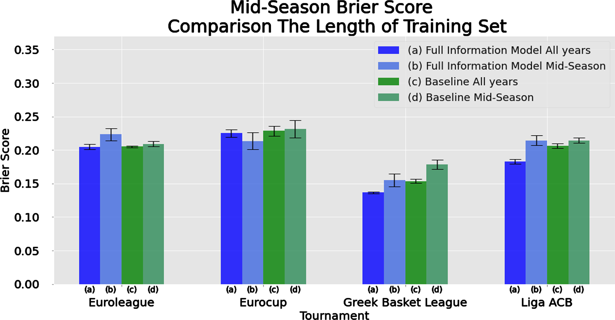
From Figure 10 (and Figure J.4 in Appendix J), we observe that the larger training data-set improves the predictive performance for the two national basketball leagues under study (Greek and Spanish) and the mid-season scenario (in terms of all measures we consider, i.e. Brier score, accuracy and F1-score) while the variability of the predictions across the different classification models is very small. Therefore, for these two leagues, the historical features offer valuable information which considerably improves predictions, possibly due to the performance of each team remaining constant across time. Moreover, the fact that all methods provide similar predictions implies that collecting more data for these two leagues is more important than selecting an “optimal” classification model. The use of extended historical data-set in the picture is the same for both models (Baseline Vanilla Model and Full Information Model) with the latter being better using either of the two training data-sets.
The situation is different for the two European basketball tournaments. For the Eurocup, the larger training data-set seems to deteriorate the prediction quality of the Full Information Model (for all metrics) while it slightly improves the prediction performance of the Baseline Vanilla Model. For the Euroleague, the larger training data-set considerably improves the prediction quality of the Full Information Model (for all metrics), while for the Baseline Vanilla Model the differences are minor (with the different metrics giving conflicting results about the predictive performance under the two training data-sets).
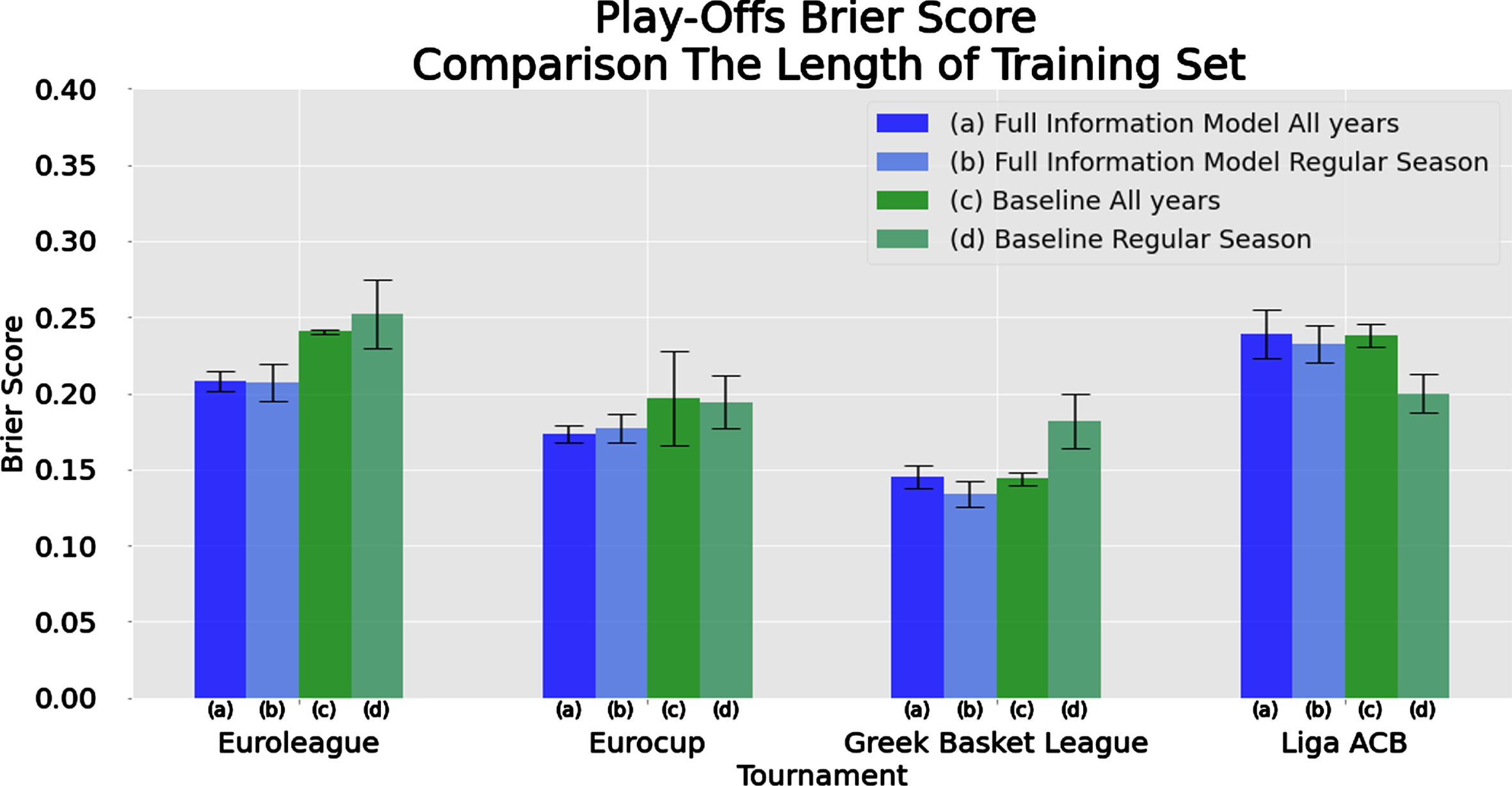
For the play-offs prediction scenario, the results are mixed. In general, the Full Information Model seems to perform better in terms of Brier score. Nevertheless, for national leagues (Greek and Spanish), the Baseline Vanilla Model also provides competitive predictions. The Baseline Vanilla Model for the Greek league using all historic data is identical (but slightly worse in terms of Brier score) than the Full Information Model using only the current regular season data. Moreover, the Full Information Model does not earn any additional value, in terms of prediction, by the use of additional historic data. Hence, in this specific case, the Baseline Vanilla Model needs more data than the Full Information Model to reach a similar prediction level, while for the Full Information Model the features from additional seasons do not seem to be relevant, since the predictive performance of this model does not improve.
For the Spanish league, the play-offs results are totally different. The Baseline Vanilla Model based only on the data of the current season outperforms all other implementations (which are of the same level in terms of Brier score). For Euroleague and the Eurocup, the Full Information Model is much better in terms of prediction than the Baseline Vanilla Model, while the use of the extensive historical data does not change dramatically the Brier score in both European tournaments. If we focus on the accuracy and F1-score, then the Full Information Model using the regular season data is better for the Euroleage while the same model is better when using the full historic data-set for the Eurocup.
As we have already mentioned in Section 4.4, in the play-off analysis, a point that needs careful treatment is the small sample size of the test dataset, which means that a surprising or outlying result in this set might greatly influence the prediction metrics. This is the reason why, in some cases, the error bars in Figure 11 indicate large variability between the different methods.
Fig. 11
Comparison of Brier score performance in the play-offs scenario for the Full Information and Baseline Vanilla Models over different tournaments/leagues and different sets of training data-set (current mid-season vs. all previous games).
4.6Feature importance
Here we present and summarize the most important features in our analysis. More specifically, we are interested in the consistency of the importance of each feature. Hence, we count how many times each feature is identified as an important determinant of the winner in each combination of classification model and type of predictive scenarios using different data-sets (full season, mid-season or play-off prediction analysis). As a result, we present the percentage of times each feature was found to be important in each of the nine different analyses (i.e. for three classifiers combined with three evaluation data-sets/scenarios). In regularized logistic regression, we consider a feature with non-zero effects are considered as important determinants of the outcome. For the other two methods (which both involve trees), a feature is considered to be important when it participates as splitting node in the fitted decision tree that improves the performance measure.
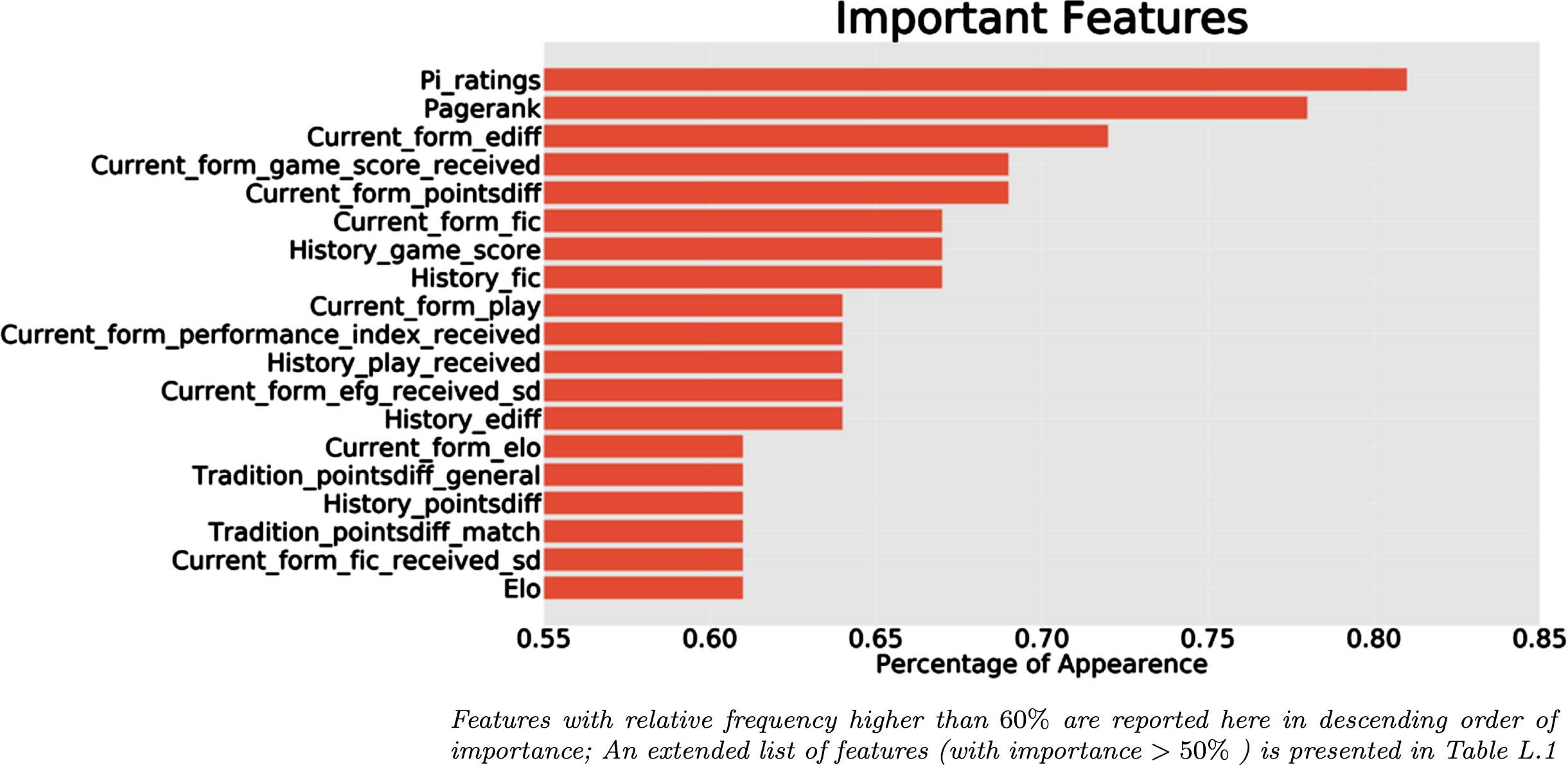
Table L.1 in Appendix L presents the percentage of importance for each feature for each tournament along with their mean percentage of importance (across the four tournaments). Features are sorted according to their overall mean importance. Only features with mean higher than 50% are included in Figure 12 depicts the overall mean importance of each feature with value higher than 60%. From this figure, it is evident that two rating systems (pi-rating and PageRank) are the most consistent important determinants of the winner. Current form measurements appear to be consistently important features for the prediction of the winner since 42% of the most important features appearing in Figure 12 are related with this characteristic. Moreover, four current form measurements follow in positions 3–6. On the other hand, five history and two tradition related measurements appear in the list of the most important features (out of 19). This might be indirectly implying that history and tradition might be less important determinants of the winner than the features related to the current form. Finally, the two ELO measurements (current form and total measurement) are marginally included in the top-list since they appear in ∼60% of the examine prediction scenarios as important determinants of the final basketball outcome.
Fig. 12
Barplot of top features according to their frequency of importance over all prediction scenarios.
5Discussion and final conclusions
Prediction of sports outcomes is a challenging task. All statistical and machine learning methods can predict the final result up to a level. Actually, the reason why sports are so attractive for fans is the uncertainty and the possibility that the weakest team or opponent can have a chance to win. In this study, we have implemented three popular statistical and machine learning techniques on basketball data from four different European leagues: two cross-country European tournaments (the Euroleague and the Eurocup) and two national ones (the Greek and the Spanish). We have focused on four different aspects:
1. Which method is better in terms of prediction?
2. Which modeling strategy or algorithm is better for prediction?
• A simple vanilla style model(which includes only the information about the competing teams and where they play), or
• a Full Information Model where a group of good features is used to boost our predictions?
3. Which data-set should be used for prediction? We have studied whether using the full historic data-set (of three years) results in better predictive models than using current season data. This was implemented in three different cases:
(a) full season prediction scenarios,
(b) mid-season prediction scenarios, and
(c) play-off prediction scenarios.
4. Which features are more consistent in terms of importance across different leagues and prediction scenarios?
5. Which league is easier to predict?
Concerning which method is better for predicting the winner in European basketball games, we can reach the following two main conclusions: (a) the overall prediction ranges from 52% to 86% in terms of accuracy, and (b) there is no clear winner between the methods since they provide identical predictions with small differences when large data-sets are used for training and learning. In this work, we have used data from three seasons in order to predict the fourth one.
We have compared two main modeling strategies for prediction. The first one is the so-called Baseline Vanilla Model which uses only the information about the two opponents and which is the home team, while the second one (Full Information Model) uses a variety of features as predictors. In general, the Full Information Model seems to outperform the Baseline Vanilla Model as expected. But the differences are lower than expected considering that we have included a lot of additional information in the form of features/predictors and the extra effort required for the analysis and the feature extraction and selection. To be more specific, the Full Information Model is better in terms of accuracy by 3 - 5% when using all previous three seasons in order to predict the last available season. The corresponding improvement is also at the same levels for the mid-season and the play-off prediction is with the exception of some limited cases (for example, in the play-offs prediction scenarios for the Spanish league and the mid-season prediction scenarios for Euroleague), where the Baseline Vanilla Model outperforms the Full Information Model in terms of accuracy.
The main reason that the two modeling strategies have similar performance, is that most of the information about the winning ability of a team is included in the simple approach of the vanilla model. The specific performance in each game can be recorded by box-score statistics and this will be more precise, but it seems that this variability is not as important as we might believe in some tournaments (e.g. the Euroleague). The big difference between those two approaches, is that the Vanilla model needs data from the current season, while Box-score based models use general characteristics of the basketball game and therefore, data from previous seasons can be used to efficiently train the model.
Regarding the size of the data required to set reliable predictions, we have performed analysis using full historical data and the current season data for the mid-season and the play-off prediction scenarios. For the mid-season analysis, using the full data-set results improves prediction models in four tournaments except for the full information analysis implemented for the Eurocup. For the latter, it seems that the current season data was more relevant. For the play-off analysis, using the full historic data did not lead to improved prediction, which implies that the current data might be more relevant for the prediction of the play-off games. Moreover, the data of the current season is usually well balanced, leading to efficient and accurate parameter learning and models with good prediction properties.
Concerning the feature importance, we have found the current form related features are the most relevant ones, appearing consistently in different models and implementations. The rating systems of PageRank and Pi-rating were also highly relevant features, while the third rating system metrics of ELO were found to be important in about 60% of the implementations. Finally, some features related to history and tradition between the opponent teams were also involved in our prediction models.
From this analysis, we can also reach, indirectly, some conclusions about the competitiveness of the teams participating in the corresponding leagues. Leagues or tournaments where the models achieve “better" prediction metrics are the ones with less competition and the prediction of the winner is easier. From our results, the Greek league is the less balanced tournament in terms of competitiveness, since all our models achieve better predictions (with an accuracy of 78%). This is reasonable since this league is dominated by two very powerful teams (Olympiakos and Panathinaikos). The second less balanced league is the Spanish one with an accuracy of 72% while for the two European tournaments the prediction accuracy is lower (about 69%).
Finally, future work should be focused on the prediction of the point difference or the game score itself. In this way, we will be able to incorporate enhanced information into our analysis which may lead to higher and more accurate estimation/learning about the strength of the teams and the efficiency of the features. Such models can be implemented via simple Gaussian regression models (for the point difference), by bivariate Gaussian regression models (for the score) or by using more sophisticated models based on appropriate distributions for the problem, such as the Poisson or the Binomial. Moreover, we can further incorporate historical data or information by using prior distributions within the Bayesian framework, which will possibly lead to models of improved prediction accuracy.
Supplementary material
[1] The Appendix section is available in the electronic version of this article: https://dx.doi.org/10.3233/JSA-220639.
References
1 | Ballı, S. & Özdemir, E. , (2021) , A novel method for prediction of euroleague game results using hybrid feature extraction and machine learning techniques, Chaos, Solitons&Fractals 1162: 111119. |
2 | Breiman, L. , (2001) , Random forests, Machine Learning 45: , 5–32. |
3 | Brier, G.W. et al., (1950) , Verification of forecasts expressed interms of probability, Monthly Weather Review 78: (1), 1–3. |
4 | Cai, W. , Yu, D. , Wu, Z. , Du, X. & Zhou, T. , (2019) , A hybrid ensemblelearning framework for basketball outcomes prediction, PhysicaA: Statistical Mechanics and its Applications 528: , 121461. |
5 | Carlin, B. P. , (2005) , Improved ncaa basketball tournament modelingvia point spread and team strength information, in Anthology ofStatistics in Sports, SIAM 149–153. |
6 | Chen, T. & Guestrin, C. , (2016) , Xgboost: A scalable tree boostingsystem, in, Proceedings of the nd acm sigkdd internationalconference on knowledge discovery and data mining 785–794. |
7 | Constantinou, A. C. & Fenton, N. E. , (2013) , Determining the level ofability of football teams by dynamic ratings based on the relative discrepancies in scores between adversaries, Journal ofQuantitative Analysis in Sports 9: (1), 37–50. |
8 | Epstein, E. S. , (1969) , A scoring system for probability forecasts ofranked categories, Journal of Applied Meteorology 8: (6), 985–987. |
9 | Fan, R.-E. , Chang, K.-W. , Hsieh, C.-J. , Wang, X.-R. & Lin, C.-J. , (2008) , Liblinear: A library for large linear classification, the, Journal of Machine Learning Research 9: , 1871–1874. |
10 | Friedman, J. H. , (2001) , Greedy function approximation: a gradientboosting machine, Annals of statistics1189–1232. |
11 | García, J. , Ibáñez, S. J. , De Santos, R. M. , Leite, N. & Sampaio, J. , (2013) , Identifying basketball performance indicators in regular season and playoff games, Journal of human kinetics 36: , 161. |
12 | Giasemidis, G. , 2020, Descriptive and predictive analysis of euroleague basketball games and the wisdom of basketball crowds, arXiv preprint arXiv:2002.08465. |
13 | Gilovich, T. , Vallone, R. & Tversky, A. , (1985) , The hot hand inbasketball: On the misperception of random sequences, Cognitive Psychology 17: (3), 295–314. |
14 | Harville, D. A. & Smith, M. H. , (1994) , The home-court advantage: Howlarge is it, and does it vary from team to team? The AmericanStatistician 48: (1), 22–28. |
15 | Hastie, T. , Tibshirani, R. , Friedman, J. H. & Friedman, J. H. , (2009) , The elements of statistical learning: data mining, inference, and prediction, Vol. 2, Springer. |
16 | Heit, E. , Price, P. C. & Bower, G. H. , (1994) , A model for predictingthe outcomes of basketball games, Applied Cognitive Psychology 8: (7), 621–639. |
17 | Hollinger, J. , (2002) , Pro Basketball Prospectus, Potomac Books. |
18 | Hollinger, J. , (2005) , Pro Basketball Forecast, Potomac Books. |
19 | Horvat, T. , Job, J. & Medved, V. , (2019) , Learning to predict soccer results from relational data with gradient boosted trees, Machine Learning 108: , 29–47. |
20 | Hubáček, O. , Šourek, G. & Železný, F. , (2019) , Learning to predict soccer results from relational data withgradient boosted trees, Machine Learning 108: , 29–47. |
21 | Hvattum, L. M. & Arntzen, H. , (2010) , Using elo ratings for matchresult prediction in association football, InternationalJournal of Forecasting 26: (3), 460–470. |
22 | Kohavi, R. & John, G. H. , (1997) , Wrappers for feature subsetselection, Artificial Intelligence 97: (1-2), 273–324. |
23 | Kubatko, J. , Oliver, D. , Pelton, K. & Rosenbaum, D. T. , (2007) , Astarting point for analyzing basketball statistics, Journal of Quantitative Analysis in Sports 3: (3), 2007. |
24 | Lazova, V. & Basnarkov, L. , (2015) , Pagerank approach to ranking national football teams, arXiv preprint arXiv:1503.01331. |
25 | Li, B. , Friedman, J. , Olshen, R. & Stone, C. , (1984) , Classification and regression trees (cart), Biometrics 40: (3), 358–361. |
26 | Lin, C.-J. , Weng, R. C. & Keerthi, S. S. , 2007, Trust region newton methods for large-scale logistic regression, in Proceedings of the 24th international conference on Machine learning, pp. 561–568. |
27 | Loeffelholz, B. , Bednar, E. & Bauer, K. W. , (2009) , Predicting nba games using neural networks, Journal of Quantitative Analysis in Sports 5: (1). |
28 | Milanović, D. , Selmanović, A. & Škegro,, D. , 2014, Characteristics and differences of basic types of offenses in european and american top-level basketball, in 7th International Scientific Conference on Kinesiology, pp. 400. |
29 | Murphy, A. H. , (1973) , Hedging and skill scores for probability forecasts, Journal of Applied Meteorology and Climatology 12: (1), 215–223. |
30 | Naismith, J. , (1941) , Basketball: Its Origin and Development, New York, Association Press. |
31 | Oliver, D. , (2004) , Basketball on paper: rules and tools for performance analysis, Potomac Books, Inc. |
32 | Page, L. , Brin, S. , Motwani, R. & Winograd, T. , 1999, The pagerank citation ranking: Bringing order to the web., Technical report, Stanford InfoLab. |
33 | Schwertman, N. C. , McCready, T. A. & Howard, L. , (1991) , Probability models for the ncaa regional basketball tournaments, The American Statistician 45: (1), 35–38. |
34 | Shi, Z. , Moorthy, S. & Zimmermann, A. , 2013, Predicting ncaab match outcomes using ml techniques-some results and lessons learned, in ECML/PKDD 2013Workshop on Machine Learning and Data Mining for Sports Analytics. |
35 | Smith, T. & Schwertman, N. C. , (1999) , Can the ncaa basketballtournament seeding be used to predict margin of victory? TheAmerican Statistician 53: (2), 94–98. |
36 | Stefani, R. T. , (1980) , Improved least squares football, basketball, and soccer predictions, IEEE Transactions on Systems, Man, and Cybernetics 10: (2), 116–123. |
37 | Torres, R. A. , 2013, Prediction of nba games based on machine learning methods, University of Wisconsin, Madison. |
38 | Van Rijsbergen, C. J. , (1979) , Information Retrieval, 2nd edition, Butterworths. |
39 | Zimmermann, A. , (2016) , Basketball predictions in the ncaab and nba: Similarities and differences, Statistical Analysis and DataMining: The ASA Data Science Journal 9: (5), 350–364. |


