
Identifying Pacing Profiles in 2000 Metre World Championship Rowing
Abstract
The pacing strategy adopted by athletes is a major determinants of success during timed competition. Various pacing profiles are reported in the literature and its importance depends on the mode of sport. However, in 2000 metre rowing, the definition of these pacing profiles has been limited by the minimal availability of data. Purpose: Our aim is to objectively identify pacing profiles used in World Championship 2000 metre rowing races using reproducible methods. Methods: We use the average speed for each 50 metre split for each available boat in every race of the Rowing World Championships from 2010-2017. This data was scraped from www.worldrowing.com. This data set is publicly available (https://github.com/danichusfu/rowing_pacing_profiles) to help the field of rowing research. Pacing profiles are determined by using k-shape clustering, a time series clustering method. A multinomial logistic regression is then fit to test whether variables such as boat size, gender, round, or rank are associated with pacing profiles. Results: Four pacing strategies (Even, Positive, Reverse J-Shaped, and U-Shaped) are identified from the clustering process. Boat size, round (Heat vs Finals), rank, gender, and weight class are all found to affect pacing profiles. Conclusion: We use an objective methodology with more granular data to identify four pacing strategies. We identify important associations between these pacing profiles and race factors. Finally, we make the full data set public to further rowing research and to replicate our results.
1Introduction
Across “closed-loop” design sports, competitions where athlete(s) attempt to complete a set distance in the shortest time (Abbiss and Laursen, 2008), different pacing strategies have been identified. Most of these pacing strategies have been defined in running and cycling races and attempts have been made to define these strategies in 2000m rowing (Garland (2005); Kennedy and Bell (2003); Muehlbauer and Melges (2011); Muehlbauer and Melges (2011)). However, these attempts approach the problems in a different manner and come to different conclusions. We attempt to standardize the definition of pacing profiles in rowing by using more granular data than other studies. The more granular data provides the opportunity to more accurately and objectively classify similar pacing profiles
Determining optimal pacing profiles can be done using ergometric data (Kennedy and Bell, 2003) or by using observational data from actual competitions (Garland (2005); Muehlbauer and Melges (2011); Muehlbauer et al. (2010)).
Kennedy and Bell (2003) used simulated rowing and training results to suggest that there were different optimal race profiles for different genders. They found that a constant pacing profile was optimal for men and an all-out profile was optimal for women. Garland (2005) used observational data from the 2000 Olympics, 2001 World Championship, and 2001 & 2002 British indoor Rowing Championship competitions. The analysis found that when using four time splits measured every 500 metres that men and women show no difference in their observed pacing strategies. Garland (2005) eliminated races that showed signs of slowdowns from the analysis. They did so because they wanted to only include boats that finished their race in the fastest time possible. Muehlbauer et al. (2010) and Muehlbauer and Melges (2011) used the same type of split time data to model pacing profiles. In 2010 they found that gender, round of race (whether race was in qualifying heat or the final race for the category), size of boat, coxed, and scull did not affect pacing strategies for the 2008 Olympics. In 2011 they had a different finding that indicated that round of race affected pacing profiles in World Championship races between 2001 and 2009. They performed these analyses by fitting linear quadratic models to the four timesplits.
1.1Types of pacing profiles
In other fixed distance cycling and running races, six pacing profiles have been defined (Abbiss and Laursen, 2008). The six profiles are “negative”, “all-out”, “positive”, “even”, “parabolic-shaped”, and “variable pacing”.
A negative-split pacing profile is defined by an increase in speed across splits (which result in smaller relative split times as the race progresses) and is often used in middle-distance events (20km cycling for example). An all-out profile is used when it is believed that energy reserves are best distributed at the start of the race. This is commonly found in shorter events like the 100 metre sprint. A positive pacing profile is one where the athletes’ speed decreases through each split in the event. This is often found in swimming (100-m and 200-m), where the diving start allows athletes to reach their maximum speed quickly. Even pacing profiles are categorized by a relatively small portion of the race spent in the acceleration phase and the majority of the race at a constant pace.
According to Abbiss and Laursen (2008), there are three pacing sub-strategies for Parabolic-Shaped pacing profiles. J-Shaped, Reverse J-shaped, and U-shaped. In general these strategies follow a parabolic shape where the middle of the race sees the lowest relative speeds. In the U-shaped strategy, the start and end of the race see the same relative speed. The J-Shaped strategy has a greater relative speed at the end of the race while the Reverse J-Shaped profiles have a greater relative speed at the start of the race. The last profile mentioned is “Variable Pacing”. It is a strategy that is used to adapt to changing conditions in the race course, like uphills and downhills in cycling.
The classification of pacing profiles has historically been approached by fitting linear models to split times (Garland (2005); Muehlbauer and Melges (2011); Muehlbauer et al. (2010)). We believe that using more granular data describing a boat’s speed throughout the race will be able to paint a better picture of how the boat is performing throughout the race. We also believe that using a clustering technique to classify similarly shaped speed curves together will provide a novel approach to defining pacing profiles.
There is a large body of literature in clustering and the area of longitudinal clustering is growing. In sports specifically, model-based clustering has been used to cluster player trajectories in basketball (Miller and Bornn, 2017), football (Chu et al., 2019), and soccer (Gregory, 2019). The previous works leverage the flexibility of model-based clustering to work across multiple dimensions to group similar shapes across time together. Their probabilistic framework is convenient for handling outliers. They also do not require a fixed specification of shape types allowing the data to speak for itself. This approach would be novel for rowing pacing profiles as previous works imposed structure on the pacing profiles. The previous works demonstrate that clustering with sufficiently granular data can help discover the underlying structures of a given dataset.
Longitudinal clustering is an emerging area of research and has been applied across fields for shape based clustering problems. McNicholas et al. (2012) used a model-based clustering approach that uses mixtures of multivariate t-distributions with a linear model for the mean and a modified Cholesky-decomposed covariance structure to cluster gene expressions over time. Additionally, Kumar and Futschik (2007) used a soft clustering technique to cluster the shapes of microarray data. Finally, using UCR time-series datasets (Chen et al., 2015), to test clustering techniques and improve the clustering techniques that are published, Paparrizos and Gravano (2016) developed the k-shape clustering technique for time series data. Good performance on the UCR time-series datasets is the gold standard for applied time-series techniques.
The objectives of this paper are twofold. Firstly, objectively determine the different types of racing strategies that are most frequently employed in rowing using more granular data. Secondly, investigate how the strategies were used in different race scenarios.
2Methods
2.1Athletes and event
We gathered GPS data from www.worldrowing.com for the average speed and stroke rate (SR) at each 50 metre split for each boat in every race of the Rowing World Championships from 2010-2017 (the years which were available when we collected data). This includes both lightweight and open races, men, women, and mixed-gender races, boat category, and all other race descriptors. Additionally, data was extracted that described the boats. We also collected finishing place, and lane data. For example, the discipline of the race is important as it is a different type of rowing style. Sculling describes a boat where rowers use two oars and Sweep describes boats where rowers have only one oar each. In Table 1 we present the number of boats by year. Note that in 2012 and 2016 only non-Olympic events were held since these were Olympic years.
Table 1
Number of Boats from each World Championship
| Year | Men | Women | Total |
| 2010 | 498 | 250 | 748 |
| 2011 | 911 | 467 | 1378 |
| 2012 | 765 | 424 | 1189 |
| 2013 | 759 | 387 | 1146 |
| 2014 | 776 | 466 | 1242 |
| 2015 | 1112 | 632 | 1744 |
| 2016 | 235 | 112 | 347 |
| 2017 | 772 | 383 | 1155 |
2.2Data Analysis
Data was initially filtered to eliminate races with GPS errors where the reported average speed is lower than the true average speed, with an unreported average speed at any of the split measurements (at every 50 metres), average speed less than two metres per second, with boats that received “Did not Starts”, “Did not Finishes” or “Exclusions”. We did not consider data from para-rowing races in the analysis. This reduced the number of boats’ races from 9264 to 8054. To determine pacing profiles raw speeds at each split are often compared to the mean speed of a boat throughout the race Garland (2005). So we define xi,j, as the speed at split i for boat j and normalize to get yi,j, where
(1)
By normalizing the speed we can compare the pacing profile of different boats while accounting for the difference in speeds. Clustering was used to group speed curves of similar shape together. In k-shape clustering a new distance method, called “Shape-based distance (SBD)”, and a new method for computing centroids are used. When SBD is evaluated against other distance metrics such as Dynamic Time Warping, it reaches similar error rates on the UCR datasets but with shorter computation times. The k-shape algorithm is implemented in the dtwclust package (Sarda-Espinosa, 2018). In its implementation it normalizes the columns to the same scale. So it takes yi,j defined in Equation (ref eq:1) and transforms it into zi,j defined as
We fit a multinomial logistic regression with pacing profile as a dependent variable on the boat size, race placement in a heat or final, discipline, gender, and weight class variables. We reported the odds ratio for each variable in the model. An effect is determined to be a statistically significant if the p-value from the Wald z-test is smaller than 0.05 divided by 39 (accounting for multiple comparisons via a Bonferroni correction) (Dunn, 1961).
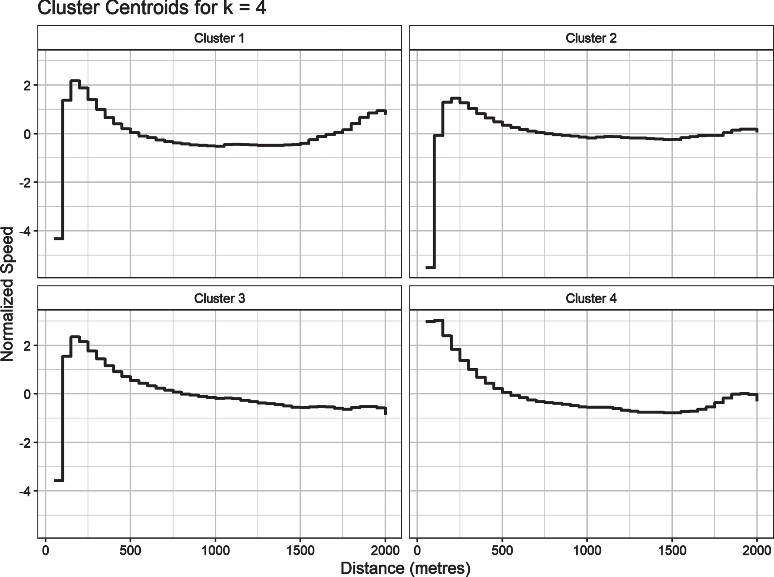
Fig. 1
Cluster Centroids for k-Shape Clustering with 4 Clusters.
3Results
3.1Comparison of pacing profiles
We performed k-Shape clustering for k = 3, 4, 5, 6, and 7. We found that k = 4 gave us the most distinct shapes, created the largest decreases in within group distances from each cluster center and corresponds to the elbow of the often used elbow method heuristic(Thorndike, 1953). The k-Shape clustering algorithm converges, which means there is an iteration of the algorithm where cluster memberships do not change, for our given seed.
To understand the shape of the clusters, we plot the centroids for each cluster in Figure ref :cluster_centroids. The centroids are similar, as expected in an all-race average; however, there are distinct features that separate them. The centroids are plotted with respect to the normalized speed by race (yi,j), in order to identify the shape of the pacing curve without the effect of magnitude that size of boat, weight class, and other variables would affect.
We will now name the clusters based on the definitions given by Abbiss and Laursen (2008).
Cluster 1, n = 1951 is defined by a slow acceleration to a moderate peak velocity, a slow middle section, and a final sprint that almost reaches peak velocity. This agrees with the definition of the U-Shaped pacing profile.
Cluster 2, n = 2277 is defined by a slower acceleration, a smaller peak velocity, and a low variance in speed throughout the rest of the race. This agrees with the definition of the Even pacing profile.
Cluster 3, n = 2548 is defined by an acceleration to top speed in the first 150 metres and a decline in speed for every proceeding split. This agrees with the definition of the Positive pacing profile.
Cluster 4, n = 1444 is defined by a quick acceleration to a higher peak velocity, a slower middle portion of the event, and finally a faster push to the finish. This agrees with the definition of the Reverse J-Shaped pacing profile.
3.2Pacing profiles and race factors
The results of the multinomial logistic regression can now help us unpack how race variables impact the use of each pacing profile discovered during our clustering process. The results of the multinomial logistic regression are reported in Table 3.
To explain how to interpret the table we will use the boat size variable as an example. There are no results reported for the “Even” pacing profile as it is used as our baseline level. Additionally, we used single sculling boats as the baseline for the boat size variable, hence the estimates are relative to these categories.
Table 2
Odds ratio changed by each variable holding all others constant. Statistically significant entries are bolded
| Positive | Reverse J-Shaped | U-Shaped | |
| Intercept | 0.8972 | 0.7654 | 1.4110 |
| Size: One-person (baseline) | – | – | – |
| Size: Two-person | 0.4795 | 0.3802 | 0.6796 |
| Size: Four-person | 0.1272 | 0.1360 | 0.1607 |
| Size: Eight-person | 0.0356 | 0.0757 | 0.0354 |
| Round of Race: Final (baseline) | – | – | – |
| Round of Race: Heat | 1.8120 | 1.037 | 0.5397 |
| Race Placement: 1st Place (baseline) | – | – | – |
| Race Placement: 2nd Place | 0.8631 | 1.020 | 1.2070 |
| Race Placement: 3rd Place | 1.0780 | 1.3260 | 1.4980 |
| Race Placement: 4th Place | 1.3580 | 1.6040 | 1.6000 |
| Race Placement: 5th Place | 1.7600 | 1.9280 | 1.2420 |
| Race Placement: 6th Place | 3.1620 | 3.1600 | 1.2050 |
| Discipline: Sculling (baseline) | – | – | – |
| Discipline: Sweep | 1.8140 | 1.2010 | 1.9660 |
| Gender: Men (baseline) | – | – | – |
| Gender: Women | 1.8830 | 1.6830 | 1.6630 |
| Weight Class: Lightweight (baseline) | – | – | – |
| Weight Class: Open | 1.4320 | 1.5230 | 1.2840 |
The odds that eights would follow a “Positive” pacing profile over a “Even” pacing profile is 0.03 times as large as those of a single sculling boats holding all other variables constant (p-value < 1e-16). We can see that all odds ratios for the eights are less than 1 indicating that eights are more likely to exhibit an “Even” pacing profile than singles are (all p-values < 1e-16).
Holding all other variables constant, the “Positive” pacing profile is nearly 2 times more likely to be used than an “Even” pacing profile in a heat than a final (p-value 2e-16). The U-shaped profile is nearly 2 times less likely to be used than an “Even” profile in a heat than a final (p-value <1e-16)
The pacing profile seems to have an effect on a given boat’s placement in the race. The baseline in this case is boats that came in first place. The question is whether this would affect how the boats would pace themselves. There is no significant difference between pacing profiles chosen by first and second place boats (p-values, Positive: 0.14, Reverse J-Shaped: 0.87, U-Shaped: 0.06). Third place boats have a similar distribution but are more likely to have a “U-Shaped” pacing profile (p-values, Positive: 0.46, Reverse J-Shaped: 0.02, U-Shaped: 0.0001). 4th place boats were more likely to follow both the Reverse J-Shaped and U-Shaped profiles (p-values, Positive: 0.0029, Reverse J-Shaped: 0.000096, U-Shaped: 0.00001). 5th and 6th place boats are significantly more likely to follow the Positive (largest p-value: 7e-8) and Reverse J-Shaped profiles (largest p-value: 1e-7).
Rowing is classified into two disciplines, Sculling and Sweep. We see that “Positive” and “U-Shaped” pacing profiles are more likely in Sweep boats than Sculling boats (p-value 9e-14 and 2e-14 respectively).
Women were statistically less likely to follow “Even” pacing profiles when accounting for all other variables included in the model. “Positive” pacing profiles were seen relatively most often for women when compared to men (p-value < 1e-16).
The “Open” weight class also saw a different distribution of pacing profiles compared to the “Lightweight” class after accounting for the other variables. Holding the other variables constant the “Positive” (p-value: 3e-8) and “Reverse J-Shaped” (p-value: 3e-8) pacing profiles were more likely to be used.
4Discussion
4.1Type of pacing profiles
The bigger the boat the more likely one was to observe an “Even” pacing profile. This is most likely because it takes a lot of inertia for the bigger boats to get moving. In order for the boat to increase its speed the rowers would need to exert power proportional to the cube of the drag force. Therefore, it is harder for larger boats with more people, such as an eight, to adjust speed mid-race. Put simply, once at a high speed it’s harder for an eight to speed up.
It was noted above that the “Positive” pacing profile is nearly two times more likely to be used in a heat than a final. This would make sense as boats that are in heats are more likely to want to conserve their energy for their future races. Anecdotally, boats will often race the first half of the race as planned and then reassess their effort if they should back off to conserve energy for the next round based on their placing at that moment (Garland, 2005). This behaviour propagates from the slowest boats to the fastest. Once the fastest boats are ahead (usually by some margin) they will react based on the slower boats’ strategy; hence contributing to higher odds of using “Positive” racing strategy. However, slowing down to conserve energy is against the FISA rules (FIS, 2019) so publicly speaking about this strategy or overtly slowing downs risks disqualification.
We also found that placing in the last three places to be statistically significant to the pacing profile used. One explanation could be that in most races the first three boats are the ones to qualify for the next race. As discussed above, once the placing is secured (especially in heats) you begin to conserve energy. Third and fourth place boats are usually battling for a qualifying spot. So, the top 2 and bottom 2 boats displayed similar strategies. Unfortunately, looking for an interaction between the race placement and the round of the race would require more data than we have available, so we leave this for further investigation.
Sweep boats were more likely than sculling boats to exhibit “Positive” and “U-Shaped” pacing profiles. This aligns with what we see in the raw race data. Sculling boats are more consistent (smaller average standard deviation of speeds through 500m to 1500m) than their sweep counterparts when comparing boats of the same size (2 sculls against 2 sweeps and 4 sculls against 4 sweeps). The reason for this difference in consistency could be due to the competitiveness of the different disciplines. Sculling races are often thought to have deeper more competitive fields (Good, 2004). If, when going into a race, a boat believes that the field is relatively even they may opt for a more conservative and balanced start (and may exhibit an “Even” or “Reverse J-Shaped” profile). Whereas, if a boat believes that it is outmatched by its competition, it may be more likely to attempt a faster start with a higher chance of fatiguing later in the race, thus exhibiting a “Positive” or “U-Shaped” profile. Both men and boats from the light weight class were associated with a greater chance of following the “Even” pacing profiles. This conflicts slightly with the findings of Garland that there were no differences in pacing profile between men and women (Garland, 2005); although, it is important to note that we used a higher resolution of data and different approaches. We are hesitant to conjecture why there are these effects and believe a more in-depth study is needed to determine why we found this association.
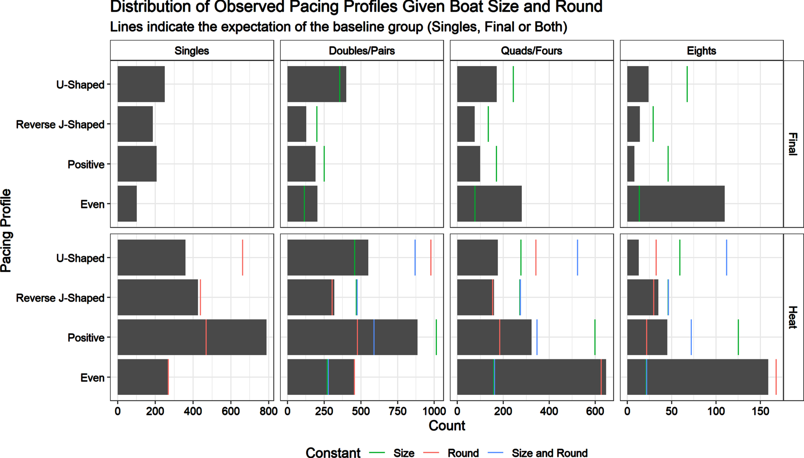
Finally, in Figure 2 we illustrate some of the strong associations we see between the size of the boats, the round of the race and the pacing profile used. When compared proportionally it is striking to see how much more often the “U-shaped” profile is used in Finals compared to Heats (1.8 times more likely than an “Even profile”, p-value < 1e-16) and how drastically the Positive profile usage drops in Finals compared to Heats (0.5 times as likely as an “Even” profile, p-value 2e-16). It is also easy to see the large difference in frequency for “Even” profiles in large boats. To further show the impact of each variable we plot the expected number of boats using each pacing profile holding size or round constant.
For example holding round constant we’d expected to see 500 boats (indicated by the red line) using the “Positive” pacing profiles in single heats. However, we observe nearly 800 of them. A more complex example considers the blue lines which adjusts both size and round to their baseline categories. For example, if the heats for Eights were the same as finals for Singles we’d expect to see nearly 110 “U-Shaped” pacing profiles in the heats for Eights. However, we’ve estimated that “U-Shaped” usage is nearly half as likely as “Even” usage in heats than finals (p-value < 1e-16) and 0.03 times for Eights compared to Singles (p-value < 1e-16). In reality, we observe 13 boats rather than the 110 expected in that category.
Fig. 2
Distribution of Observed Pacing Profiles Given Boat Size and Round. Coloured lines indicate the expectation of the baseline group.
It is important to note that we are not inferring any causal relationships between the variables as we are studying observational data. We are at risk to have unmeasured confounders and sampling bias due to variable interactions. Additionally, we do not currently account for the interaction between boats during the race. We are only able to measure the exhibited pacing profile not the desired or intended pacing profile. These are all areas for improvement and future research.
5Conclusion
Our approach makes an important contribution to the current literature. We provide an objective, data-driven approach to quantifying racing strategy. Previous analyses have been done through a subjective quantification. This approach uses a complex time series clustering method to characterize racing strategies. With these clusters, we developed a model which allows inference to be made about these racing strategies in relation to other factors present during a race. The granularity of the data we provide is what allows the methods we have presented to make accurate classifications. Furthermore, the granular data collected has been made available to the public so that future analyses may be performed with similar accuracy.
Acknowledgments
We would like to thank Dr. Dave Clarke for organizing this partnership between Simon Fraser University and Canadian Sport Institute Pacific, Chuck Rai for his incredible help with scraping data, and Lucas Wu and Kevin Floyd for their consultations on statistics and rowing strategies. We would also like to thank Ron Yurko, Sam Ventura, Rebecca Nugent, and the Carnegie Mellon Sports Analytics Club for hosting the reproducible research competition that pushed us to make our work reproducible and available to the public.
References
1 | (2019). FISA RULE BOOK. Federation Internationale des Societes dAviron. |
2 | Abbiss C. R. , Laursen P. B (2008) , Describing and understandingpacing strategies during athletic competition, Sports Medicine(Auckland, N.Z.), 38: , 239–52. |
3 | Chen Y. , Keogh M. , Hu E. , Begum N. , Bagnall A. , Mueen A. , Batista G. 2015, The UCR Time Series Classification Archive. |
4 | Chu, D. , Reyers, M. , Thomson, J. , Wu, L. Y. (2019) , Routeidentification in the national football league, Journal of Quantitative Analysis in Sports, 0: (0). |
5 | Dunn, O. J. (1961) , Multiple comparisons among means, Journal ofthe American Statistical Association 56: (293), 52–64. |
6 | Garland S. W. (2005) , An analysis of the pacing strategy adopted byelite competitors in 2000 m rowing, British Journal of SportsMedicine, 39: (1), 39–42. |
7 | Good M. (2004) , The sculling crisis, Rowing News, 11: (5), 4251. |
8 | Gregory S. 2019, Ready player run: Off ball run identification and classification. In Proceedings of the2019 Barca Sports Analytics Summit. |
9 | Kennedy M. D. , Bell G. J. (2003) Development of race profilesfor the performance of a simulated 2000-m rowing race, CanadianJournal of Applied Physioligy 28: (4), 536–546. |
10 | Kumar L , Futschik M. 2007, Kumar l, futschik e.. mfuzz: a software package for soft clustering of microarray data. bioinformation 2:5-7. Bioinformation, 2, 5–7. |
11 | Lloyd S. P. (1982) , Least squares quantization in pcm, IEEETransactions on Information Theory 28: , 129–137. |
12 | McNicholas P , Sanjeena , Subedi (2012) , Clustering geneexpression time course data using mixtures of multivariatet-distributions, Journal of Statistical Planning andInference 142: , 1114–1127. |
13 | Miller A.C. , Bornn L. 2017, Possession sketches : Mapping nba strategies. In Proceedings of the 2017 MIT Sloan Sports Analytics Conference. |
14 | Muehlbauer T. , Melges T. (2011) , Pacing patterns in competitiverowing adopted in different race categories, The Journal ofStrength & Conditioning Research 25: . |
15 | Muehlbauer T. , Schindler C. , Widmer A. (2010) , Pacing patternand performance during the 2008 olympic rowing regatta, European Journal of Sport Science, 10: (5), 291–296. |
16 | Paparrizos J. , Gravano L. , (2016) , k-shape: Efficient andaccurate clustering of time series, SIGMOD Record, 45: (1), 69–76. |
17 | Sarda-Espinosa A. 2018, dtwclust: Time Series Clustering Along with Optimizations for the Dynamic Time Warping Distance,R package version 5.5.0. |
18 | Thorndike R. (1953) , Who belongs in the family? Psychometrika, 18: (4), 267–276. |


