
Exploring the potential of the plus/minus in NCAA women’s volleyball via the recovery of court presence information
Abstract
This work describes a collaboration with a single collegiate volleyball team to leverage existing data to examine the potential of the plus/minus metric for player evaluation. Historically, volleyball players have been evaluated through a series of single skill metrics (e.g., number of aces per set and hitting percentage). The advantages of the plus/minus lie in the limited amount of information needed for its calculation (e.g., court presence and scoring) combined with its ability to fuse together both measured and unmeasured contributions. Unfortunately, the primary collection tool (Statcrew) for National Collegiate Athletic Association (NCAA) Women’s Volleyball, does not record the movement of the Libero, resulting in incomplete court presence information for a large percentage of plays. This paper introduces methodology to recover court presence information from standard play-by-play data. The recovery is in the form of a posterior distribution of player presence, which can then be used to not only calculate the plus/minus metric but also quantify the uncertainty of the metric due to the incomplete information. Although the presented methods and results were derived from a collaboration with a single team, the data source and methodology can be extended to multiple teams.
1Context and problem
The role of the keyer on the game day stat crew for a college volleyball team is to enter the live call of the statistician into the computer software program Statcrew. These data are compiled into summary statistics for the coaches, media, and record keeping. One author, who served as a keyer, noticed that not every action taken by players is recorded (e.g., block retained by blocker’s team) and not every recorded action translated into a traditional statistic (e.g., failed dig). Because of this, the author approached team staff to see about using these data to construct the plus/minus metric in the hopes of gaining useful player insights.
The plus/minus has persisted as a tool for player evaluation since the late 1960’s in ice hockey and has more recently become popular in basketball. In its basic form, plus/minus is the points scored by a player’s team minus the points scored by the opposing team when that player is in the game. Kubatko et al. (2007) briefly describes its history in professional basketball and how it entered the official record for the National Hockey League as early as the 1967–68 season (2016a). More recent advances in this methodology describe the use of penalized regression models to construct an adjusted plus/minus that controls for the other players on the court and other contextual factors (Gramacy et al., 2013, Macdonald, 2012).
Focusing on net points accumulated during a player’s time in the game gives this metric the potential to combine various measured skills as well as capture certain intangible qualities that a player provides such as defensive ability. Defensive contributions are under-represented in many sports by traditionally available data. Schatz (2005) points out this deficiency in football statistics and Franks et al. (2015) discuss this issue in basketball.
The focus on net points scored also places players on a common basis of comparison, regardless of role on the team. This contrasts with current metrics in volleyball which focus on the performance of or relative value of single measurable skills. Metrics are not comparable across positions simply due to each player’s assigned responsibilities. Individual performance of actions is interwoven with and dependent upon the actions of teammates, which traditional metrics do not capture. For example, a team that passes well will put the setter in a much better position than one that does not, but they may both record an equal number of digs. Examples of work focusing on single skills include how setters respond to blocking formations (Araújo et al., 2010), the importance of the speed of sets (Fellingham et al., 2013), what affects the type and quality of serves (Quiroga et al., 2012), and how to optimize service error rates (Burton & Powers, 2015). Other work has taken a more general approach examining the relative importance of in-game actions by linking skills to the probability of scoring (Florence et al., 2008, Miskin et al., 2010) or to winning (Claver Rabaz et al., 2013, Eom & Schutz, 1992). The literature is devoid, however, of attempts to quantify player contribution in terms that are comparable across position or in ways that account for actions that do not involve touching the ball like the plus/minus.
Although the plus/minus and its derivatives have generally been applied to sports with a continuous nature of play, such as basketball, hockey, and soccer (Hamilton, 2014, Vilain & Kolkovsky, 2016), there is nothing in the methodology that precludes its use from sports such as volleyball. In fact, the discrete structure of volleyball makes data processing more straightforward than that described by Macdonald (2011). In volleyball, each play contains a point won or lost and the players in the game remain fixed for that play. The average squad carries 15–16 players (Irick, 2015) and up to 15 substitutions per set is allowed (Pufahl, 2016). This often results in a variety of on-court rosters making player performance differentiation possible.
The difficulty in implementing a plus/minus for volleyball lies in the Libero position. The Libero is a designated player restricted to the back row and whose substitutions do not count against the cap. For this reason the movement of the Libero on and off the court is not recorded in Statcrew. This means that for a majority of plays there is incomplete court presence information.
This paper describes the collaboration with a collegiate volleyball team to assess the utility of adjusted plus/minus metrics for player evaluation using these incomplete data. The remainder of the paper is organized as follows. In Section 2, the available data are detailed in terms of format and processing. Section 3 details the method proposed to impute the missing information. Section 4 examines the accuracy of this approach. Section 5 gives various plus/minus results followed by a discussion of the findings and potential future directions.
2Estimation of incomplete data
The primary data collection instrument for college volleyball is a program called Statcrew (2016b). Each home team provides the output of the program to the NCAA for official record keeping. A by-product of the program is a text file that contains play-by-play codes for each game. For example, each play begins with a serve and ends with either a block (point won while on defense), kill (point won while on offense), or error (point lost). This makes it possible to track which team scored on each play. In addition, the file consists of a majority of actions of each play. This includes the type of contact and who performed it. For example, the play output D:1 S:20 K:13 indicates that Player #1 dug the ball (first offensive touch), Player #20 set it (second offensive touch), and Player #13 attacked receiving a kill (hit the ball over the net and scored a point). Other information in the output allows one to track substitutions.
What is not recorded, however, is the movement of the Libero. The Libero is a special position, typically a defensive specialist, who is free to replace players in the back row without counting against the substitution cap. When the opposing team is serving (service out), the Libero can replace any player in the back row. When the team is serving (service in), the Libero is permitted to serve in place of one of the players in the serving rotation and can replace the other two back row players in the other five rotations. Due to the unrecorded movements of the Libero, it is often not possible to know the complete court presence information required for a plus/minus calculation. Inferring whether the Libero is on the court and if so, which player is replaced, is necessary to calculate an accurate plus/minus.
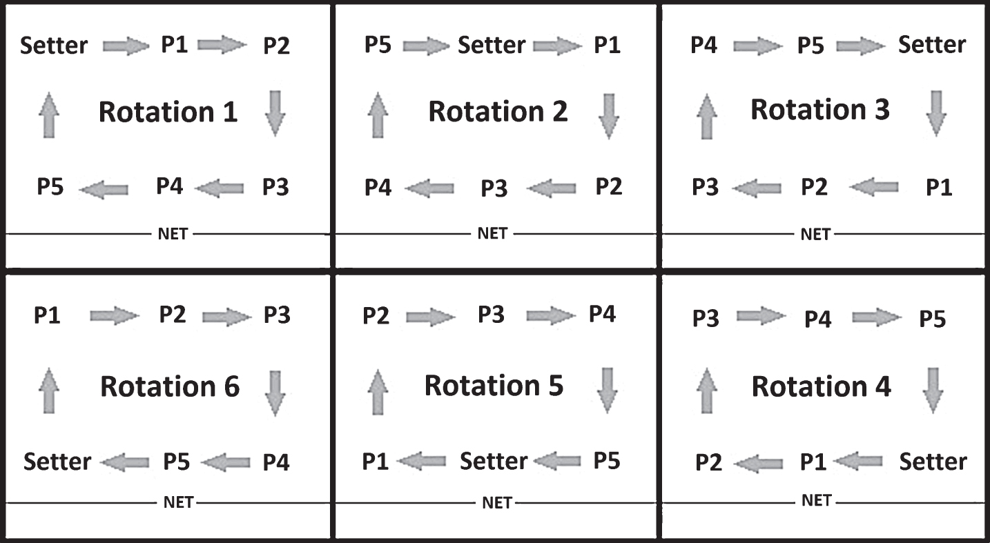
This inference can be done by first using the rules of the game and the data from Statcrew to determine which players are, or might be, on the court. In volleyball, six players per team occupy six predefined spots on the court. The rules require three players to occupy the front row and three to occupy the back row. The player in the back left (as viewed with one’s back to the net) is the server and continues to serve until the other team scores a point. When the team regains the serve, each player rotates one spot clockwise as pictured in Fig. 1.
Fig. 1
Player Rotation in Volleyball. Each box represents half the court with the bottom of the box being the net. The figure demonstrates the designation of players to the front and back row over the series of serve rotations. Positions on the court are described from the perspective of standing with one’s back to the net. P1-P5 stand generically for Players 1, 2, 3, 4, and 5, while the setter is the player whose role is to pass the ball to attacking players.
In Statcrew, the six starters and the Libero for each game of a match are listed, as well as each substitution. This allows us to know which seven players might be on the court, but not the positions they occupy. The positions can be determined through the service order. For example, if Player #1 serves first for their team, Player #2 serves second, and Player #3 serves third it is known that Player #1 began in the back row left spot, Player #2 began in the front left, and Player #3 in the front middle. Sometimes a player who starts does not serve. In that case the substitution information must be used. For example, if Player #8 were to sub into the game for Player #4 and then serves 4th, it is known that Player #4 began the game in the front right spot. An R script (available upon request) was written to handle most of this data processing automatically.
To illustrate how court presence information is derived from the raw data consider the unprocessed sample output in Table 1 from the Statcrew program (line numbers have been added for clarity and player numbers have been altered). The starters for the visiting and home teams are given on Lines 2 and 3, respectively. The last player in each row is always the Libero.
Table 1
Sample Output from Statcrew
| Line | Statcrew Text | Line | Statcrew Text |
|---|---|---|---|
| 1 | RALLY:Y | 21 | TEAM:H SERVE:8 |
| 2 | STARTERS:V,9,17,8,20,15,1,10 | 22 | D:20 S:4 K:17 |
| 3 | STARTERS:H,18,11,16,10,9,8,7 | 23 | SUB:V,13,1,,,, |
| 4 | TEAM:H SERVE:18 | 24 | TEAM:V SERVE:13 |
| 5 | D:10 S:9 A:8 | 25 | D:11 S:11 K:18 |
| 6 | D:16 S:18 A:11,E | 26 | SUB:V,3,13,,,, |
| 7 | TEAM:V SERVE:20 | 27 | SUB:H,16,15,,,, |
| 8 | D:11 S:18 K:10 | 28 | TEAM:H SERVE:16 |
| 9 | TEAM:H SERVE:11 | 29 | D:3 S:4 A:17 |
| 10 | D:9 S:10 K:1 | 30 | S:18 A:11 |
| 11 | SUB:H,15,16,,,, | 31 | S:4 A:20 |
| 12 | TEAM:V SERVE:15 | 32 | D:8 OVER: |
| 13 | D:7 S:18 A:8 B:17,8 | 33 | S:4 K:14 |
| 14 | TEAM:V SERVE:15,E | 34 | TEAM:V SERVE:10,E |
| 15 | TEAM:H SERVE:10 | 35 | TEAM:H SERVE:7 |
| 16 | D:20 S:9 K:8 | 36 | D:3 S:4 K:14 |
| 17 | SUB:V,4,8,14,9,, | 37 | SUB:V,8,4,9,14,, |
| 18 | TEAM:V SERVE:4 | 38 | TEAM:V SERVE:9 |
| 19 | D:11 S:18 K:9 | 39 | D:11 S:18 A:11 |
| 20 | TEAM:H SERVE:8,A RE:10 | 40 | D:9 S:20 A:8,E |
The first goal is to put the starting players into their spots in the rotation for the first play. For this illustration the visiting team will be used. The first step is to find the serve order by locating the first 6 lines that begin with TEAM:V SERVE: followed immediately by a unique number. Lines 7, 12, 18, 24, 34, and 38 reveal the visitor service order to be Players #20, #15, #4, #13, #10, and #9. Note that line 14 is skipped, as it is redundant information. Figure 2B shows these six players in positions according to the order in which they served. Players #17, #8, and #1 started the game but are not in this service order. We must use the sub information (Lines 17, 23, 26, and 37) and the fact that the Libero, Player #10, serves to get back to the original players on the floor at the start of the game.
Fig. 2
A: Rotation Spots on the Floor. B: Players Placed by Serve Order. C: Player Position Adjusted by Subs. D: Player Position Adjusted by Libero.
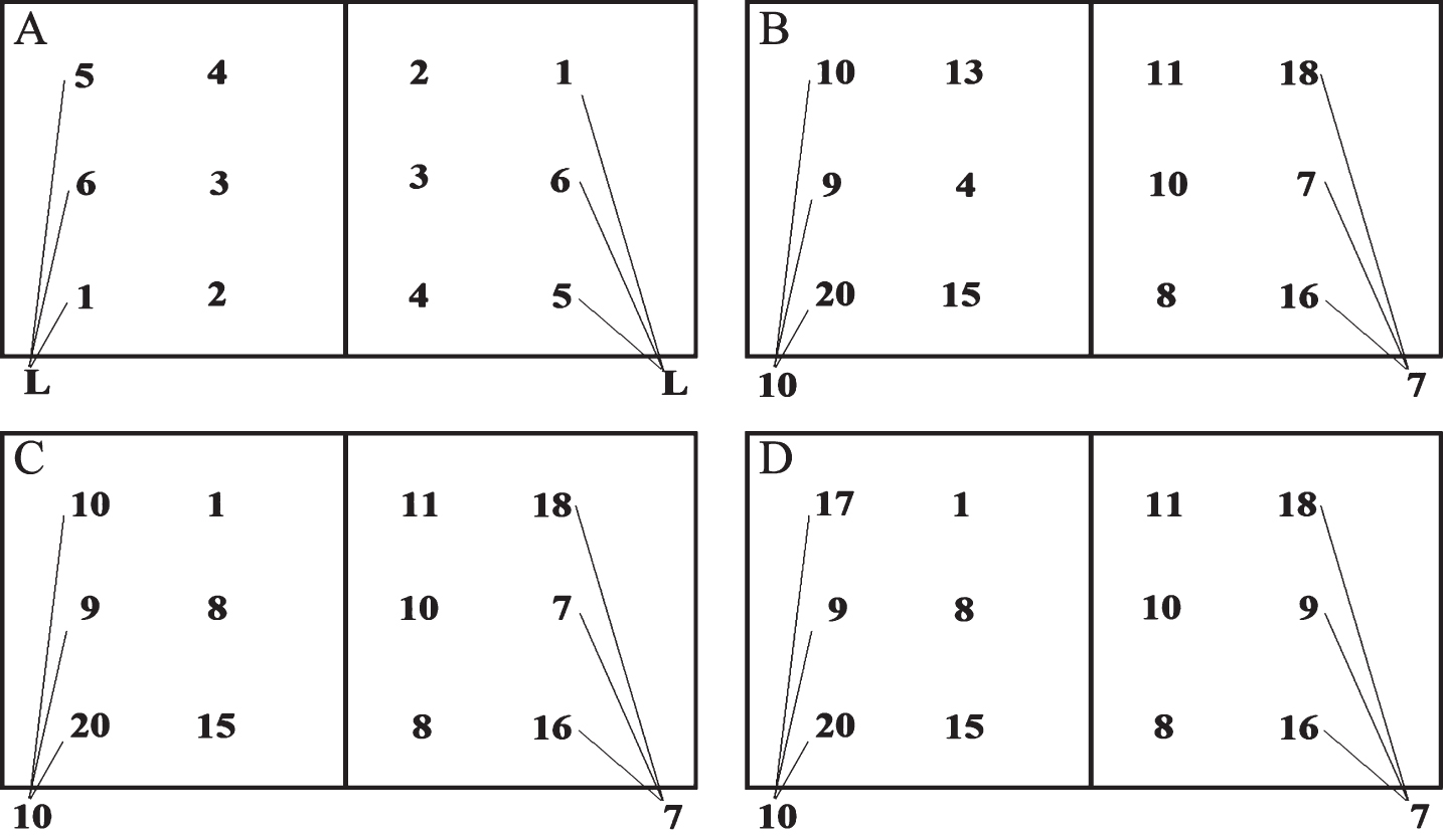
The software allows for a maximum of three substitutions per line, each entered as a player pair. The first number in the pair indicates which player came in, and the second number indicates which player was replaced. Line 17, for example, indicates that Player #4 entered the game and replaced #8, and Player #14 entered the game replacing #9. In order to use the sub information to go from serving rotation to starters, work through the substitution lines in reverse order, placing the second player in a sub pair into the rotation in place of the first. Line 37 indicates that Player #4 replaces #8 (ignored because 4 is already in the serve order) and Player #14 replaces #9 in Spot 6. Line 26 specifies that Player #13 should replace #3, this is ignored since Player #3 is not in the serve order. For Line 23, Player #1 replaces #13 in Spot 4. Lastly, in Line 17, Player #8 replaces #4 in Spot 3 and Player #9 replaces #14 in Spot 6. The players on the floor now resemble Fig. 2C. Since Player #10 is the Libero and in the service order, and Player #17 started the game, was not subbed for, and did not serve, replace #10 with #17 in Spot 3. The correct starting rotation is shown in Fig. 2D. The method is repeated for the home team, but now using lines with H instead of V.
Given the starting rotation for both teams, court presence for each play can be filled in by working through the play by play. For the remainder of the set, every time service is gained by the visiting team, visiting players are rotated one spot closer to 1 with 1 moving to Spot 6. Similarly for the home team when they gain the serve. Players are swapped in whenever their team makes a substitution. Proceeding in this fashion identifies which seven players might be in for each play. The players occupying the front row (Spots 2, 3, and 4) are known to be in by rule. Only three players out of the Libero and the players in the back row (Spots 1, 6, and 5) are in. The play-by-play data contain some indication of which of these players are in the game through their recorded actions, but the remaining plays are missing complete court presence information.
To develop and test methodology to recover this court presence information, the Statcrew output for a recent season of a Division I volleyball team is used. After processing this output as described, the data set is constructed as a 4988×16 matrix. Each row stands for a play that occurred during the season. The columns of the matrix contain indicators of which team scored as well as characteristics of the play (i.e., whether the service was in or out, which spot on the court the setter occupied, and the court presence information for each of 13 players who participated in at least one play over the course of the season). Uncertain court presence is designated as a missing value.
3Modeling court presence
Given the starting rotation, it is known which seven players may be on the court for any play. To compute the plus/minus, it is necessary to determine which three players out of four occupy the back row. This information is either known, partially known, or entirely unknown. Rather than choose the three players who are in, a model was developed to choose which of the four possible players is out. For this purpose, a Bayesian multinomial model is adopted using rotation and serve information to predict the omitted player. The resulting posterior distribution of court presence allows the computation of players’ plus/minus across the possible court presence matrices, thereby incorporating uncertainty of court presence into the plus/minus metrics.
Rather than focus on the absence of specific players, the model predicts the absence of specific spots in the rotation. Since the three front row spots are always in, only four spots need to be considered, the three back row spots and the Libero position. The absence matrix Z is defined as an N×4 matrix with elements as defined in Equation 1.
(1)
The missing elements of matrix Z need to be estimated using two sources of information.
3.1Rotation information
This source relies on the assumption that coaching substitution strategy is based on a player’s role. For example, if a player is a strong front row player, but a weak back row player, a coach will choose one of two options to keep her from being a back row liability: The coach may 1) sub her out anytime she rotates to the back row or 2) use the Libero for the same purpose. If two such players are in play simultaneously, it is possible to space them in the rotation such that only one ever appears in the back row at a time, and use the Libero for both.
A team will rotate six times before the original server returns to the service position as displayed in Fig. 1. The original position of the players on the court is called Rotation 1. When the 2nd player takes the service position, this is called Rotation 2. This proceeds up to Rotation 6 after which the players will be in their original places, or back to Rotation 1. Each rotation represents a unique decision for the coach to place the Libero in one of the back row spots or on the bench.
3.2Serve information
By NCAA rule, the Libero is permitted to occupy one spot in the service order (Pufahl, 2016). This affects the predictions for a team that has two players in their rotation who are replaced by the Libero as at least one of them will have to serve. While service is in, that player will be in the back row. Once the other team gains the serve, however, that player may be replaced by the Libero. This highlights the need to use service information to predict Libero presence.
Using the six rotations and service in or out gives 12 possible combinations to consider as predictor variables. An indicator matrix R is used to operationalize this, where each play is a row and each column indicates a rotation and service in/out combination. For example, Ri1 is Rotation 1 service in, Ri2 is Rotation 1 service out, and Ri3 is Rotation 2 service in for play i. Across games, rotations are matched based on the starting position of the setter.
For example, if the setter is in the service position, it is called Rotation 1, regardless if the other players match across games. In the example data set, the setter started every game and was therefore a reliable link across games for matching rotations. If two different setters are employed over the course of a season, simply using the one that is in provides the link. If two setters are used simultaneously, one of them should be chosen and used consistently to designate rotation. Failure to properly match rotations will lead to additional uncertainty in the estimate of court presence.
3.3Multinomial model and notation
Each row of matrix Z is assumed multinomial with four categories. The probabilities are modeled as
3.4Model estimation
Of primary interest is the posterior distribution of Z, which is a function of the posterior distribution of β. For estimation, the approach of Polson et al. (2013) is adopted. They built upon the use of auxiliary variables in Bayesian multinomial regression (Holmes & Held, 2006). Their approach introduces the Polya-Gamma (PG) random variate distribution to sample auxiliary variables (ωj), which allow for a Gibbs sampler.
To sample new β, the package BayesLogit (Windle et al., 2014) is used. Given θ, it is possible to directly sample Z (the missing court presence information), which is the primary interest. The following algorithm is adopted to sample Z.
Algorithm
0) Define:
1) Initialize
For iterations t:
2) Draw β|R, Zt-1 using BayesLogit
2a) ωt|βt-1 ∼ PG (·)
2b)
3) Draw
4) Iterate through Steps 2 and 3 saving each draw of Zt.
The initialization in Step 1 allows all rows to contribute to the initial estimates ω1, β1, and θ1. Fractional values do not cause an issue as all three estimates rely on a collapsed Z matrix for unique rows of the R matrix. Including the partial rows allows spots in particular rotation serve combinations with more missing information across plays to begin as a more likely candidate to be out. Greater detail for the distribution parameters of Step 2 are given in the Appendix. This process is run for 1000 iterations taking the first 20 draws as a burn-in as convergence occurred quickly. The remaining 980 draws can be used in two ways. First, each draw on court presence can be used to calculate plus/minus resulting in a posterior distribution of plus/minus. Second, the draws can be used to calculate the most likely court presence configuration by designating the player drawn to be out the most number of times as actually out. This is the maximum a posteriori (MAP) estimate of court presence.
4Testing the reliability of estimated court presence
In order to verify the model’s ability to recover court presence, results were compared against true court presence information. Game film was obtained for two matches and the movement of the Libero was tracked and input by hand. One game was home and one was away, against unique conference opponents. The standard plus/minus were calculated for the 12 players appearing in the two matches using the model-based approach and three naïve estimates for court presence.
If the complete court presence information is known, it is straightforward to calculate the standard plus/minus metric. Let Y be the vector of N play outcomes, 1 if a point was won and – 1 if a point was lost. Let P be the N×m player presence matrix, where the ijth element is 1 if the jth player is on the court for play i and 0 otherwise. The plus/minus calculation is simply YTP.
In this context, however, P is not completely known and must be estimated. For purposes of comparison with the model approach and for motivation to recover court presence, three naïve estimates are introduced. With complete information, ∑ Pij = 6 for each play i, so all three estimates maintain this property. They are ordered by the amount of information used / data processing required.
The first estimate splits the six spots on the court evenly amongst the seven players who might be on the court (Equation 2). This only requires tracking starters and subs. On any play, however, the players occupying the front row are known to be in, since, by rule the Libero cannot replace them. This leads to the second estimate (Equation 3), which additionally requires tracking player rotation. Finally, tracking the play data often reveals some of the back row players. This leads to the third estimate (Equation 4).
(2)
(3)
(4)
The third approach represents the most complete estimate without modeling court presence and includes two ways to arrive at complete or partially complete information for a play. First, when the Libero is serving, it is known whose spot the Libero is occupying. This provides complete presence information. Second, it is assumed the personnel on the court remains unchanged as long as the server remains unchanged and is uninterrupted by a timeout or a recorded substitution. This allows touch information across a set of plays to provide complete or partially complete information for that set of plays. For the example data set, approximately 25% of the rows are complete, and 75% have between 2–4 players that might be on the court.
The average absolute deviation errors in calculating plus/minus from the different methods across all 12 players are shown in Table 2. There is improvement in the estimates as additional information is incorporated with the Bayesian model outperforming all of them by a dramatic amount. The Maximum A Posterior (MAP) estimate in this case recovers the true plus/minus.
Table 2
Court Presence Estimation Methods Impact on Plus/Minus
| Court Presence Estimation Method | Participation | Position | Share | Bayes Model | Bayes MAP |
|---|---|---|---|---|---|
|
| 4.47 | 4.29 | 3.20 | 0.16 | 0.00 |
5Application of plus/minus metric using the court presence data
In this section, some potential player evaluation metrics using court presence are examined. The data consist of a single season’s matches (32) containing 114 sets with a total of 4,988 plays. All plays had one team in common with 25 unique opponents and 7 home and away series. This team played 13 different players with a consistent Libero and setter across all matches. In order to protect the privacy of the athletes, each player is labeled using a randomly assigned letter.
The plus/minus results from the entire season are given in Table 3 in the second column. Five versions of the adjusted plus/minus (APM), used in other sports, are shown in Columns 4 through 8. These metrics utilize regression models to adjust a player’s court presence impact for the other players on the court and various play context such as home court. The use of penalized regression (or the Bayesian equivalents) is due to multicollinearity in the player court presence data commonly found in APM models. These regression coefficients were derived from three different R packages.
Table 3
Adjusted Plus/Minus Estimates
| PLYR | Plus/minus | Plus/minus per 50 Plays | APM per 50 Plays BayesLogit | APPM per 50 Plays GLMNET Ridge | APM per 50 Plays GLMNET Elastic Net α = 0.5 | APM per 50 Plays GLMNET Lasso | APM per 50 Plays Reglogit | Plays |
|---|---|---|---|---|---|---|---|---|
| G | 300 | 3.01 | 3.63 | 3.42 | 6.33 | 7.46 | 5.62 | 4976 |
| A | 363 | 3.94 | 1.73 | 1.82 | 1.03 | 0.69 | 1.29 | 4609 |
| K | 126 | 2.86 | 0.78 | 0.78 | 0.12 | 0.03 | 0.00 | 2204 |
| I | 160 | 3.07 | 0.72 | 0.70 | 0.08 | 0.00 | 0.00 | 2608 |
| M | 0 | 0.00 | 0.66 | 0.72 | 0.13 | 0.04 | 0.00 | 18 |
| C | 64 | 2.26 | 0.57 | 0.51 | 0.00 | –0.11 | 0.00 | 1418 |
| J | 240 | 3.22 | 0.36 | 0.35 | –0.21 | –0.32 | 0.00 | 3730 |
| F | 206 | 2.85 | 0.14 | 0.19 | 0.00 | –0.32 | 0.00 | 3608 |
| B | 87 | 3.24 | 0.00 | 0.05 | –0.16 | –0.49 | 0.00 | 1343 |
| L | 8 | 6.06 | –0.70 | –0.64 | –1.29 | –1.75 | 0.00 | 66 |
| D | 74 | 1.52 | –1.01 | –0.92 | –1.59 | –1.94 | 0.00 | 2430 |
| E | 82 | 3.06 | –1.11 | –1.01 | –1.73 | –2.09 | 0.00 | 1342 |
| H | 54 | 1.71 | –1.30 | –1.21 | –1.90 | –2.25 | 0.00 | 1576 |
Each row represents a player from the team studied for a single season. Each column is a measurement from the season. APM stands for adjusted plus/minus. Plays include MAP estimate for missing data.
The five penalized regression models can be broken down by the choice between the lasso and ridge penalties and the choice between Bayesian and frequentist estimation methods. The lasso penalty adds the sum of the absolute value of the regression coefficients to the optimization function. This has the impact of shrinking coefficients to zero making the model more sparse, thereby highlighting particular players (Tibshirani, 1996). The ridge penalty adds the sum of the squared coefficients to the optimization function. It adds bias to the regression coefficients while reducing the variability in the estimates making them more likely to be near the true value (Hoerl & Kennard, 1970) To illustrate the difference between the two penalties, consider two players who are perfectly collinear (i.e., either both on or off the court together). The lasso penalty chooses one to be an average player (coefficient of 0) and essentially gives the credit of their combined effort to the other player. The ridge penalty splits the credit evenly between the two players. A compromise between the two is called the elastic net. The Bayesian approaches utilize a Laplace prior (lasso) or a Normal prior (ridge) on the regression coefficients to accomplish the same result. The primary advantage of the Bayesian approach is that it produces a posterior distribution for the regression estimates which allows for probability statements and measures of uncertainty. The primary advantage of the frequentist approach is that its estimation is faster and tends to be easier to implement. Examples of implementation of these models in sports are given in Sill (2010), Macdonald (2012), and Gramacy et al. (2013).
The calculation of the APM using the regression coefficients (λ) is as follows. The APM assumes an even odds context (plus/minus of 0) as the baseline. Player j is then substituted for a player with no impact such that the adjusted plus/minus per 50 plays is given by Equation 5.
(5)
The choice of 50 plays as the rate denominator is tied to the average game (or set) length in the data. The BayesLogit package fits a logistic regression with a Normal prior on the regression coefficients. GLMNET (Friedman et al., 2010) was used to fit the frequentist Ridge, Elastic Net, and LASSO penalized regression methods. Reglogit is described by Gramacy et al. (2013) and can be thought of in simplified terms as a Bayesian LASSO model, although in practice it is more complex. The two-step process they recommend was utilized for estimating a prior, which also requires the Textir package of Taddy (2013). The final column includes the number of plays in which, according to the MAP estimate, each player participated.
Given the data are from a single team, generalizability of the results are limited, however insights as to their usefulness are still possible. For example the two Lasso methods (GLMNET Lasso and Reglogit) are designed to introduce sparsity. They both agree on Player’s G and A as being the strongest, but the Lasso model had many more non-zero estimates making Reglogit preferred in that respect. The choice of G and A as the strongest passes the eye test as these are also the two players the coaching staff played the most often (almost 900 plays more than the third place player). The two ridge methods produce similar orderings. If the coefficients are the only interest, the authors prefer GLMNET for its ease of implementation. If, however, the use of the regression coefficient posterior distribution is needed for estimation of uncertainty and interesting player and roster comparisons as illustrated by Deshpande and Jensen (2016) than the authors prefer BayesLogit. In general the results from the adjusted plus/minus were found to be believable by staff with a few exceptions. Player F was seen as being rated too low given that she was considered the best at her position. Players L and M were rated by coaches to be the lowest contributors and typically only played towards the end of matches that were well in hand.
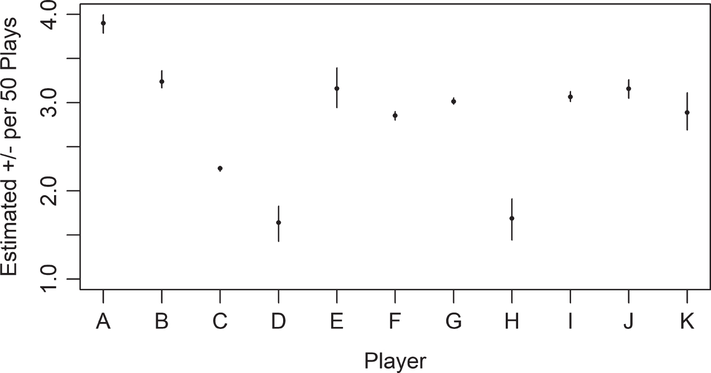
Figure 3 displays the 95% equal tailed credible intervals for player’s plus/minus, standardized to be per 50 plays, if they appeared in at least 5% of the season (249 plays). The circle gives the estimated median and the line gives the credible interval across the draws on court presence. The variability across player estimates dominates the variability within a player across draws of court presence suggesting that it may not add much to include the full posterior of court presence in future analysis with these data. This represents a meaningful reduction in estimation time. Note that all estimates are positive because the team outscored its opponents in the aggregate.
Fig. 3.
Variability in the Plus/Minus due to Court Presence Uncertainty Over a Single Season (4988 Plays).
6Conclusions
This paper describes the results of a collaboration with a single NCAA Women’s volleyball team on the usefulness of the plus/minus and adjusted plus/minus metrics in player evaluation. To get the plus/minus information, one first recovers complete court information. This is necessary because Statcrew does not track the court presence of the Libero. Court presence is estimated using a Bayesian multinomial model that assumes that the coaches are consistent in their use of roles over the course of the season. This model did well when compared to video evidence from a few games but could suffer if substitution patterns involving the Libero were to change course drastically during the year. An example of a detrimental change would be if a team went from having two middle blockers who are replaced by the Libero when rotated to the back row, to allowing one of the middle blockers to remain in the game for all six rotations. Court presence information could be estimated separately for each section of the season in this case but one would need to classify the sections manually. Failure to account for such a change would increase the uncertainty in the estimate for court presence and bias the plus/minus results calculated from it.
In the dataset used to illustrate the methodology, the variability due to court presence was dominated by the variability in the scaled plus/minus metric. This indicated that it was not necessary to use the full set of draws from the posterior distribution of court presence in subsequent analysis. This may not be the case for all such data and the analyst would be wise to check the level of uncertainty due to court presence. If it is relatively large, presenting the plus/minus metric as in Fig. 3 or sampling across the draws on court presence if estimating a Bayesian APM model is recommended.
The primary road block to creating metrics based on the Statcrew data is the inherent messiness that the program allows. For example, data inputters will sometimes fail to input a substitution as it occurs while they are still sorting out the previous play’s actions. Such errors are easy to catch automatically, but less easy to correct automatically. Access to the raw data files may also be limited. Play-by-play data are generally available through the NCAA, but these data are a derivative of the Statcrew raw files and omit much of the in-play touch information as well as some of the substitution information. This makes data processing more difficult and decreases the number of plays with complete data. Alternative data sources, such as DataVolley, that collect substitution patterns and scoring outcomes, but omit the movement of the Libero, can also utilize the presented model to recover court presence data.
This work is limited in a few ways. Primarily by the fact that all results are drawn from a single team. This limits generalizability. The use of data from multiple teams may present as yet undiscovered difficulties. The team studied was also fairly consistent in strategy and injury free which allowed for combination of data across matches with relative ease. Given the large amount of collinearity in player use in volleyball, separation in player estimates requires multiple games making this metric less useful for in-season roster adjustments.
In this particular instance, the results based on the plus/minus model were not surprising to collaborators. This was a positive in that the model was able to order players in a reasonable fashion. It was also a negative as the plus/minus results did not provide new information from their perspective. This work, however, has led to projects on other data sources which appear more fruitful. These methods require the court presence estimation model outlined in this paper, and their description is left for future work.
What makes this framework potentially useful is that the data source is already being generated for use by the NCAA. This means that the metrics illustrated are potentially scalable to the entire association. If data were to be obtained and processed for an entire conference, the use of team effects in an APM model could produce results similar to that of work done for closed leagues as in professional basketball and hockey. The plus/minus metrics provide a way to incorporate otherwise difficult to measure contributions and place all players on the same scale for comparison. Such results may be interesting from an entertainment perspective or useful for consideration of post season awards, picking national teams, or as a tool for professional teams looking to acquire new talent.
Appendices
APPENDIX
Detailed Notation from Polson et al. Model
(A1)
(A2)
The Polya-Gamma distribution shown in Equation A3, is an infinite sum of Gamma random variables. The value ni is the number of total plays the ith combination of rotation and serve occurred. The parameter ηij is equal to
(A3)
The Normal mean mj, of Equation A2, is equal to
References
1 | 2016a. 1967-68 NHL Stats [Online]. QuantHockey.com. Available: http://www.quanthockey.com/nhl/seasons/1967-68-nhl-players-stats.html. [Accessed 8-22-16 2016]. |
2 | 2016b. Statistics Policies and Guidelines. The National Collegiate Athletics Association. |
3 | Araújo, R.M. , Castro, J. , Marcelino, R. & Mesquita, I.R. (2010) , Relationship between the opponent block and the hitter in elite male volleyball, Journal of Quantitative Analysis in Sports, 6. |
4 | Burton, T. & Powers, S. (2015) , A linear model for estimating optimal service error fraction in volleyball, Journal of Quantitative Analysis in Sports 11: , 117–129. |
5 | Claver Rabaz, F. , Jiménez Castuera, R. , Gil Arias, A. , Moreno Domiguez, A. & Moreno Arroyo, M.P. (2013) , Relationship between performance in game actions and the match result. A study in volleyball training stages, Journal of Human Sport and Exercise, 8. |
6 | Deshpande, S.K. & Jensen, S.T. (2016) , Estimating an NBA player’s impact on his team’s chances of winning, Journal of Quantitative Analysis in Sports 12: , 51–72. |
7 | Eom, H.J. & Schutz, R.W. (1992) , Statistical analyses of volleyball team performance, Research quarterly for exercise and sport 63: , 11–18. |
8 | Fellingham, G.W. , Hinkle, L.J. & Hunter, I. (2013) , Importance of attack speed in volleyball, Journal of Quantitative Analysis in Sports 9: , 87–96. |
9 | Florence, L.W. , Fellingham, G.W. , Vehrs, P.R. & Mortensen, N.P. (2008) , Skill evaluation in women’s volleyball, Journal of Quantitative Analysis in Sports, 4. |
10 | Franks, A. , Miller, A. , Bornn, L. & Goldsberry, K. Counterpoints: Advanced defensive metrics for nba basketball. 9th Annual MIT Sloan Sports Analytics Conference, Boston, MA, (2015) . |
11 | Friedman, J. , Hastie, T. & Tibshirani, R. (2010) , Regularization paths for generalized linear models via coordinate descent, Journal of Statistical Software, 33: , 1. |
12 | Gramacy, R.B. , Jensen, S.T. & Taddy, M. (2013) , Estimating player contribution in hockey with regularized logistic regression, Journal of Quantitative Analysis in Sports 9: , 97–111. |
13 | Hamilton, H. (2014) , Adjusted Plus/Minus in football - why it’s hard, and why it’s probably useless [Online]. Soccermetrics Research. Available: http://www.soccermetrics.net/player-performance/adjusted-plus-minus-deep-analysis [Accessed 8-22-16 2016]. |
14 | Hoerl, A.E. & Kennard, R.W. (1970) , Ridge regression: Biased estimation for nonorthogonal problems, Technometrics, 12: , 55–67. |
15 | Holmes, C.C. & Held, L. (2006) , Bayesian auxiliary variable models for binary and multinomial regression, Bayesian analysis, 1: , 145–168. |
16 | Irick, E. (2015) , NCAA Sports Sponsorship and Participation Rates Report. The National Collegiate Athletic Association. |
17 | Kubatko, J. , Oliver, D. , Pelton, K. & Rosenbaum, D.T. (2007) , A starting point for analyzing basketball statistics, Journal of Quantitative Analysis in Sports, 3. |
18 | Macdonald, B. (2011) , A regression-based adjusted plus-minus statistic for NHL players, Journal of Quantitative Analysis in Sports, 7. |
19 | Macdonald, B. (2012) , Adjusted plus-minus for nhl players using ridge regression with goals, shots, fenwick, and corsi, Journal of Quantitative Analysis in Sports, 8. |
20 | Miskin, M.A. , Fellingham, G.W. & Florence, L.W. (2010) , Skill importance in women’s volleyball, Journal of Quantitative Analysis in Sports, 6. |
21 | Polson, N.G. , Scott, J.G. & Windle, J. (2013) , Bayesian inference for logistic models using Pólya–Gamma latent variables, Journal of the American Statistical Association, 108: , 1339–1349. |
22 | Pufahl, A. (2016) , Women’s Vollyeball 2016 and 2017 Rules and Interpretations. The National Collegiate Athletic Association. |
23 | Quiroga, M.E. , Rodriguez-Ruiz, D. , Sarmiento, S. , Muchaga, L.F. , Grigoletto, M.D.S. & García-Manso, J.M. (2012) , Characterisation of the main playing variables affecting the service in high-level women’s volleyball, Journal of Quantitative Analysis in Sports, 8. |
24 | Schatz, A. (2005) , Football’s Hilbert problems, Journal of Quantitative Analysis in Sports, 1. |
25 | Sill, J. Improved NBA adjusted+/-using regularization and out-of-sample testing. Proceedings of the 2010 MIT Sloan Sports Analytics Conference, (2010) . |
26 | Taddy, M. (2013) , Multinomial inverse regression for text analysis, Journal of the American Statistical Association, 108: , 755–770. |
27 | Tibshirani, R. (1996) , Regression shrinkage and selection via the lasso, Journal of the Royal Statistical Society. Series B (Methodological), 58: (1), 267–288. |
28 | Vilain, J.-B. & Kolkovsky, R.L. (2016) , Estimating individual productivity in football. |
29 | Windle, J. , Polson, N. & Scott J. (2014) , BayesLogit: Bayesian logistic regression, R package version: 0.5, 1. |

