
Classification of all-rounders in limited over cricket - a machine learning approach
Abstract
In cricket, all-rounders play an important role. A good all-rounder should be able to contribute to the team by both bat and ball as needed. However, these players still have their dominant role by which we categorize them as batting all-rounders or bowling all-rounders. Current practice is to do so by mostly subjective methods. In this study, the authors have explored different machine learning techniques to classify all-rounders into bowling all-rounders or batting all-rounders based on their observed performance statistics. In particular, logistic regression, linear discriminant function, quadratic discriminant function, naïve Bayes, support vector machine, and random forest classification methods were explored. Evaluation of the performance of the classification methods was done using the metrics accuracy and area under the ROC curve. While all the six methods performed well, logistic regression, linear discriminant function, quadratic discriminant function, and support vector machine showed outstanding performance suggesting that these methods can be used to develop an automated classification rule to classify all-rounders in cricket. Given the rising popularity of cricket, and the increasing revenue generated by the sport, the use of such a prediction tool could be of tremendous benefit to decision-makers in cricket.
1Introduction
An all-rounder in cricket is a player who is capable of performing well at both batting and bowling. These all-rounders still have their dominant role by which one categorizes them as batting all-rounders or bowling all-rounders. To the knowledge of authors of this paper, currently, there is no precise method for a player to be categorized as a bowling all-rounder or a batting all-rounder. Therefore, the current practice of accomplishing this tends to be very much subjective. In this paper, authors attempt to find a precise method to categorize all-rounders using machine learning techniques. A review of the literature on the problem including a brief introduction to cricket is presented in the next section.
1.1What is cricket?
Cricket is a field game played between two teams. Each team consists of eleven players that include several batsmen, several bowlers, and a wicket keeper. Cricket matches are played on a grass field, in the center of which is a flat strip of ground 20 m long and 3 m wide called the pitch. At both ends of the pitch, 20 m apart, wickets are placed. A wicket, usually made of wood, is used as a target of the bowler. The bowler bowls the ball from one end of the pitch, and the batsman who is on the other end (striker) tries to hit the ball with the bat while protecting his wicket. Once a batsman hits the ball sufficiently far, he runs to the (non-striker) wicket while the other batsman at the non-striker wicket simultaneously runs to the striker wicket, accumulating a single run. Manage and Scariano (2013) provides more details about scoring and other aspects of cricket.
There are three main types of cricket games, namely test cricket, One Day International (ODI), and Twenty20, which is rapidly becoming popular among cricket fans. In a cricket game, before play commences, the two team captains toss a coin to decide which team shall bat or bowl first. The captain who wins the toss makes his decision on the basis of tactical considerations, based on ground conditions and the strengths and weaknesses of the two teams.
1.2One day international (ODI) cricket
An ODI cricket match is played on a single day. Each team gets only one innings, and that innings is restricted to 50 overs (six deliveries per over). In an innings, each bowler is restricted to bowling a maximum number of overs equal to one fifth (10 overs in ODI) of the total number of overs in the innings. If ten batsmen are out before the end of the 50th over, the innings is also over. Note that the batsmen play as pairs and as soon as the 10th batsman is out, the last batsman does not have a partner to play. Even if the first team’s innings ends in this manner, the second team still has all of its 50 overs to score the required runs. If the second team passes the score before they run out of the resources (overs or wickets), then it wins the match. On the other hand, if the second team runs out of resources before it reaches the target, the first team wins the match.
It is the responsibility of the selectors to strategically choose batsmen, bowlers, and a wicket keeper based on both teams– strengths and weaknesses. Furthermore, as we mentioned, each team must have at least five players who are capable of bowling. Cricket captains usually change the bowlers around to introduce variation and to prevent the batsmen building longer innings and partnerships. For this, even though a team must consist of a minimum of five bowlers, team captains usually take advantage of having more than five players to bowl during an innings. Consequently, team selectors place particular emphasis on having several players who can excel in both batting and bowling.
1.3All-rounders
An all-rounder is a player who is capable of contributing to the team by both bat and ball as needed. Having several capable all-rounders in a team is a great asset to the captain. While it is not uncommon to have all-rounders as top-order batsmen, they usually play in the middle order. Their task is to carry on the momentum built by the top-order batsmen or to take control of building the innings if the top-order batsmen collapse early. Even though all-rounders are good at both batting and bowling, they still have their dominant role by which we categorize them as batting all-rounders or bowling all-rounders. In some situations, this classification can be a challenging task. To best of our knowledge, there is no standard method to do this classification. The goal of this paper is to determine an appropriate method for classifying all-rounders into bowling all-rounders or batting all-rounders, based on their performance parameters.
1.4Applications of machine learning in cricket
Machine learning is becoming popular in statistical data analysis, especially as a classification technique. It has the potential to predict both game outcomes and player performance in cricket. Given the rising popularity of cricket, and the increasing revenue generated by the sport, the use of machine learning as a prediction tool could be of tremendous benefit to decision-makers in cricket.
Several studies have used machine learning techniques and other related statistical procedures for prediction and classification in sports. Saikia and Bhattacharjee (2011) used stepwise multinomial regression and naïve Bayes classification models to classify all-rounders in the Indian Premier League (IPL) tournament. In that article, the authors suggested four different classifications of cricket players as performer, underperformer, batting all-rounder, and bowling all-rounder. Akhtar and Scarf (2012) suggested a method to forecast the outcome probabilities of test matches using a sequence of multinomial logistic regression models. Davis et al. (2015) provided a methodology to investigate both career performances and current form of the players in Twenty20 cricket. Asif and McHale (2016) developed a dynamic logistic regression (DLR) model for forecasting the winner of ODI cricket matches at any point of the game. Pathak and Wadhwa (2016) used modern classification techniques such as naïve Bayes, support vector machines, and random forest to conduct a comparative study to predict the outcome of ODI cricket. Agarwal et al. (2017) have considered factors for the selection of 11 players from a pool of 16 players, based on relative team strengths between the competing teams. Jayalath (2018) discussed a machine learning approach to analyze ODI cricket games. Jayanth et al. (2018) proposed a supervised learning method using the SVM model with linear, polynomial, and RBF kernels to predict the outcome of cricket matches. They also introduced a player ranking system using the performance statistics. Khan et al. (2019) used logistic and log-linear regression models to explore the association of influential factors with match results of ODI cricket games. Wickramasinghe (2020) discussed a naïve Bayes approach to predict the winner of an ODI cricket game.
There have been numerous studies that apply machine learning techniques and other related methods in other sports data as well. Ofoghi et al. (2013) discussed the utilization of an unsupervised machine learning that assist cycling experts in the crucial decision-making processes for athlete selection, training, and strategic planning in the track cycling. Leung and Joseph (2014) presented a sports data mining approach to predict outcomes in sports such as college football. Rein and Memmert (2016) discussed how big data and modern machine learning technologies aid in developing a theoretical model for tactical decision making in team sports. Baboota and Kaur (2019) created a feature set for determining the most important factors for predicting the results of a football match using feature engineering and exploratory data analysis. They also created a highly accurate predictive system using machine learning. Thabtah et al. (2019) proposed a new intelligent machine learning framework for predicting game results in the National Basketball Association (NBA) by aiming to discover the influential features that affect the outcomes of NBA games. Yi and Wang (2019) used the advantages of machine learning techniques in data analysis and feature mining in the training of dragon boat sports. They proposed a machine learning-based safety mode control model for dragon boat sports physical fitness training. Cust et al. (2019) reviewed the literature on machine and deep learning for sport-specific movement recognition using inertial measurement units and computer vision data inputs. By analyzing some recent research on sports prediction, Bunker and Thabtah (2019) have also shown that machine learning techniques such as artificial neural network can be used as a prediction and classification technique in sports data.
2Data set
We have included 149 players (all-rounders) in our study, most of whom are currently playing in international games. We have also included some players who have recently retired from international cricket to improve the applicability of our conclusions. Out of these, 83 were bowlers (bowling all-rounders) and 66 were batsmen (batting all-rounders). This was based on the categorization from the respective teams (countries). There were some players for whom that categorization was not listed. For those cases, we have searched through expert match commentaries and decided the category based on those expert comments. We have separated the data set into two sets, using random assignment as usual. Consequently, 112 players (75%) were used in model building; that was called the training data set. The remaining 37 players (25%) were set aside as the testing data set to validate the models. In the training data set, there were 62 bowlers and 50 batsmen. The testing data set consisted of 21 bowlers and 16 batsmen.
Classification of all-rounders is done based on their performance statistics. The authors have carefully selected the following statistics to accomplish this task.
X1- Runs: Total number of runs scored by the player
X2- Batting Average: Total number of runs a batsman has scored divided by the total number of times he has been called out
X3- Batting Strike Rate: The number of runs scored per 100 balls faced by a batsman
X4- Wickets: The number of wickets taken by a bowler
X5- Bowling Average: The average number of runs conceded per wicket by a bowler X6- Economy Rate: The average number of runs conceded per over by a bowler
X7- Bowling Strike Rate: The average number of balls bowled per wicket taken by a bowler
Runs scored, batting average, and batting strike rate are batting statistics, for which a higher value indicates better performance. The number of wickets taken, bowling average, economy rate, and bowling strike rate are bowling statistics. Better performance is indicated by higher values for wickets taken, and lower values for the other three bowling statistics. As shown in Table 2.1, for the data set we considered, mean batting averages respectively for batting all-rounders and bowling all-rounders were 33.74 and 15.42. This indicates that a batting all-rounder scores 18.32 runs more than a bowling all-rounder on average. The batting strike rate for batting all-rounders was 87.63, while the same for bowling all-rounders was 76.32. This indicates that a batting all-rounder scores 11.31 runs more per hundred balls on average. The mean bowling averages for batting all-rounders and bowling all-rounders were 48.78 and 32.45 respectively. This shows that a batting all-rounder conceded 16.33 more runs per wicket on average. Based on mean bowling strike rates, we see that a typical batting all-rounder uses 14.68 more balls per wicket than a bowling all-rounder. Economy rates indicate that a batting all-rounder concedes 0.33 more runs per over on average. These statistics can be used as reference guidelines as we try to derive an automated classification mechanism for classifying all-rounders.
Table 2.1
Descriptive Statistics of Performance Parameters
| Variable | Cat | N | Mean | StDev | Median |
| Runs | bat | 66 | 3680.00 | 3024.00 | 2657.00 |
| bowl | 83 | 593.80 | 895.30 | 284.00 | |
| Batting Average | bat | 66 | 33.74 | 9.26 | 33.81 |
| bowl | 83 | 15.42 | 8.24 | 14.33 | |
| Batting Strike Rate | bat | 66 | 87.63 | 12.79 | 86.92 |
| bowl | 83 | 76.32 | 18.89 | 78.39 | |
| Wickets | bat | 66 | 45.24 | 49.78 | 30.50 |
| bowl | 83 | 99.59 | 72.29 | 82.00 | |
| Bowling Average | bat | 66 | 48.78 | 27.01 | 41.95 |
| bowl | 83 | 32.45 | 7.02 | 31.13 | |
| Economy Rate | bat | 66 | 5.44 | 0.54 | 5.38 |
| bowl | 83 | 5.11 | 0.50 | 5.04 | |
| Bowling Strike Rate | bat | 66 | 53.03 | 24.47 | 47.20 |
| bowl | 83 | 38.35 | 9.01 | 35.50 |
Furthermore, due to the nature of the predictor variables in our study, they usually have some inherited dependency among them. To overcome issues like multicollinearity that arise due to this dependency, we have converted these predictor variables to principal components and those principal components were used as the new predictor variables with model building. The first five principal components explain 97.6% of the total variability, and they can be expressed as linear combinations of the original predictors as below;
L1 = 0.369X1 + 0.438X2 + 0.226X3 - 0.287X4 + 0.487X5 + 0.290X6 - 0.466X7
L2 = 0.403X1 + 0.456X2 - 0.518X3 + 0.319X4 - 0.354X5 - 0.178X6 - 0.321X7
L3 = -0.373X1 - 0.043X2 - 0.370X3 + 0.442X4 + 0.209X5 - 0.600X6 - 0.351X7
L4 = -0.393X1 + 0.255X2 - 0.578X3 - 0.540X4 - 0.282X5 - 0.069X6 - 0.264X7
L5 = -0.286X1 - 0.045X2 - 0.345X3 + 0.529X4 + 0.023X5 - 0.703X6 - 0.152X7
Next section presents results along with a brief introduction to the six different classification techniques that we used.
3Classification methods - different machine learning approaches
In this study, we have applied six different techniques that are being commonly used by practitioners for classification, to classify all-rounders into bowling all-rounders or batting all-rounders based on their performance parameters. Those techniques are:
(1) Logistic Regression (LR)
(2) Linear Discriminant Analysis (LDA)
(3) Quadratic Discriminant Analysis (QDA)
(4) Naíve Based Classifier (NB)
(5) Support Vector Machine (SVM)
(6) Random Forest (RF)
To quantify the performance of the different classification methods, we used two evaluation metrics; the first was accuracy, in which the classification strength is evaluated at a specific threshold. This is, in fact, the rate of correct classification based on that threshold. The second metric was the Area Under Curve (AUC) of the Receiver Operating Characteristic (ROC) curve, which is a more comprehensive measure. It is a tradeoff between the true positive rate and false positive rate of a particular classification method. AUC is a more aggregate measure that gives an overall summary of the performance based on multiple thresholds. Therefore, it is known that the AUC outranks accuracy measures when quantifying the performance of classification techniques. Nevertheless, we present the results of both accuracy and AUC for each of the six classification methods. Both of these measures were calculated for the training sample as well as for the testing sample. Performance based on testing sample is essential to evaluate the robustness of the techniques.
3.1Logistic regression
Logistic Regression is a machine learning technique that is commonly used for classification. It is highly used in binary classification problems. A binary logistic regression model was fitted by taking the player’s grouping (bat or ball) as the response variable. The predicted probability of the ith player under the model developed by using the 112 players in the training data set is given by;
For the training sample, out of the 62 bowlers, the model misclassified 2 players (Mohammad Saifuddin and Imad Wasim). Out of the 50 batsmen, 4 were misclassified (Hardik Pandya, Dwayne Smith, Moises Henriques, and Mominul Haque). This gave a correct classification rate of 94.64% with an area under the ROC curve 0.9829. To assess the robustness, the model was used to predict the class of the players in the testing sample. Out of the 21 bowlers, none were misclassified. Furthermore, out of the 16 batsmen, 3 were misclassified (Dasun Shanaka, Stuart Binny, and Corey Anderson). The confusion matrix for logistic regression along with other confusion matrices for the rest of the techniques are provided in the Appendix. The model gave a correct classification rate of 91.89%, with an area under the curve 0.9912 for the testing sample. Fig. 4 shows the ROC curve for the testing sample.
3.2Linear discriminant analysis
Linear Discriminant Analysis (LDA) is another simple and effective method for classification. LDA is commonly used as a dimensionality reduction technique as well. As a classification technique, LDA creates the axes for best class separability. The LDA algorithm divides the data into output categories using linear boundaries based on the given predictor variables. As usual, here we used the training sample to build the LDA classification function. The predictive performance was evaluated based on both training and testing samples.
In the training sample, out of the 62 bowlers, 4 were misclassified (Mohammad Saifuddin, James Faulkner, Andile Phehlukwayo, and Imad Wasim). Out of the 50 batsmen, 3 were misclassified (Dwayne Smith, Moises Henriques, and Mominul Haque). The model gave a correct classification rate of 93.75%, with an area under the curve 0.9729. In the testing sample, out of the 21 bowlers, only Andre Russell was misclassified. Furthermore, out of the 16 batsmen, none were misclassified. The correct classification rate for the testing sample was 97.3%, with an area under the curve 0.9792. Fig. 5 shows the ROC curve for testing sample.
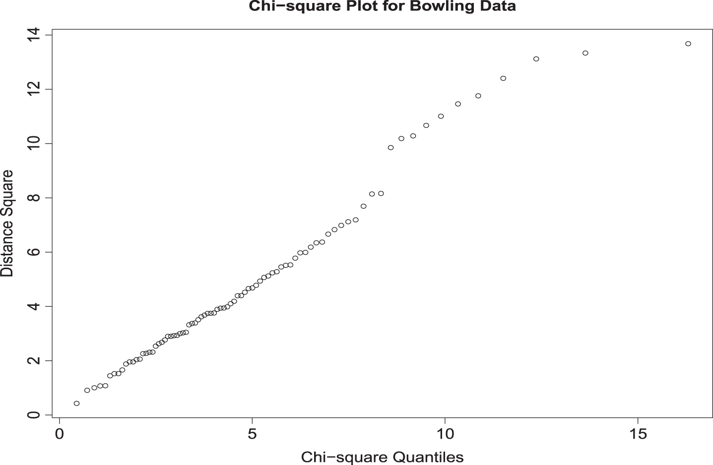
The assumption of normality is required for both LDA and QDA methods. Chi-square plots for batting and bowling data in Fig. 1 and 2 do not indicate any serious violations of this assumption. Homogeneity of the covariance matrices is an assumption for the LDA method. Box–s M test indicated that (Approximate chi-square value = 241.06 with degrees of freedom = 15) the two covariance matrices are not the same. However, since the Box–s M test is highly sensitive to normality, it not uncommon to see such outcomes.
Fig. 1
Chi square Plot for Batting Data.
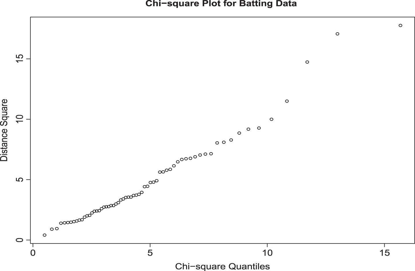
Fig. 2
Chi square Plot for Bowling Data.
3.3Quadratic discriminant analysis
Quadratic Discriminant Analysis (QDA) is an extension of Linear Discriminant Analysis. QDA is more flexible than LDA and it is applied when the within-class covariance matrices are not equal. The flexibility is achieved due to the relaxation of the assumptions in the covariance structure of the classes. However, it requires a substantial amount of computation due to the large number of parameter estimations. The discriminant function for the QDA is given by;
Si : Sample covariance matrix of the ith category
pi : Prior probability that the observation belongs to the ith category
The classification is done by categorizing the player in the category that gives the highest value of
In the training sample, the QDA model misclassified 4 out of the 62 bowlers (Seekkuge Prasanna, Mohammad Saifuddin, Andile Phehlukwayo, and Mohammad Nabi). Out of the 50 batsmen, 8 were misclassified (Hardik Pandya, Moeen Ali, Dwayne Smith, Moises Henriques, Nasir Hossain, Colin Grandhomme, Mosaddek Hossain, and Mominul Haque). Consequently, the model correctly classified 89.29% of the players, giving an area under the curve 0.9645. In the testing sample, the model correctly classified all 21 bowlers and only one of 16 batsmen was misclassified (Dhananjaya de Silva). The model possessed high robustness, giving a correct classification rate of 97.30%, with an area under the curve 0.9970 for the testing sample. Fig. 6 shows the ROC curve for testing sample.
As shown in the previous section, the assumption of normality can be verified by the chi-square plots(Fig. 1 and 2). Box–s M test results (Approximate chi-square value = 241.06 with degrees of freedom = 15) show that the covariance matrices are not equal which is the second assumption that should be satisfied for the QDA method.
3.4Naïve Bayes classifier
Naïve Bayes is a probabilistic machine learning technique based on Bayes Theorem. It uses the probabilistic approach to classify a data set. Naïve Bayes assumes that the predictor variables of the classes are independent. Although this is a strong assumption, it is true in our data set, as our predictor variables are independent, being the principal components. In our data set, each feature variable Li, i = 1, 2, 3, 4, 5 comes from a class of conditional Gaussian distribution
and Cj, j = 1, 2. Here C1 and C2 are the two classes (batting and bowling).
Given the prior P (C), the decision rule using the Naive Bayes approach is given by;
When we applied Naïve Bayes Classifier to the training sample, it misclassified 4 of the 62 bowlers (Seekkuge Prasanna, Mohammad Saifuddin, James Faulkner, and Imad Wasim) and 6 of the 50 batsmen (Elton Chigumbura, Dwayne Smith, Moises Henriques, Nasir Hossain, Colin Grandhomme, and Mominul Haque). The model had a correct classification rate of 91.07%, with an area under the ROC curve 0.9716. In the testing sample, the model incorrectly classified two of 21 bowlers (Andre Russell and Al-Amin Hossain) and 3 of 16 batsmen (Dhananjaya de Silva, Kevin O’Brien, and Stuart Binny). The model predicts the players 86.49% times correctly, giving an area under the ROC curve 0.9554. Fig. 7 shows the ROC curve for the testing sample.
3.5Support vector machine
Support Vector Machine (SVM) is a machine learning technique that can be used for classification and regression. As in the other methods, here our focus was to use SVM as a classification technique to categorize all-rounders as batting all-rounders or bowling all-rounders. The goal in SVM is to find the optimal boundary to classify a data set. SVM maximizes the margin around the hyperplane that separates the classes. The support vectors are the subset of training samples that help to specify the decision function. Depending on the nature of the data set, an analyst has to select the appropriate kernel function for SVM. The task of a kernel function is to transform the data set into a form that facilitates a linear classification. Furthermore, these kernel functions are generalizations of the dot products. The simplest one is the linear kernel, which does not need any transformation. Several other non-linear kernel functions can be applied to transform the data, such as radial bases kernel (RBF), polynomial kernel and sigmoid kernel. An Introduction to Statistical Learning with Applications in R by James et al. (2013) provides an excellent introduction to SVM and other manchine learning teachniques.
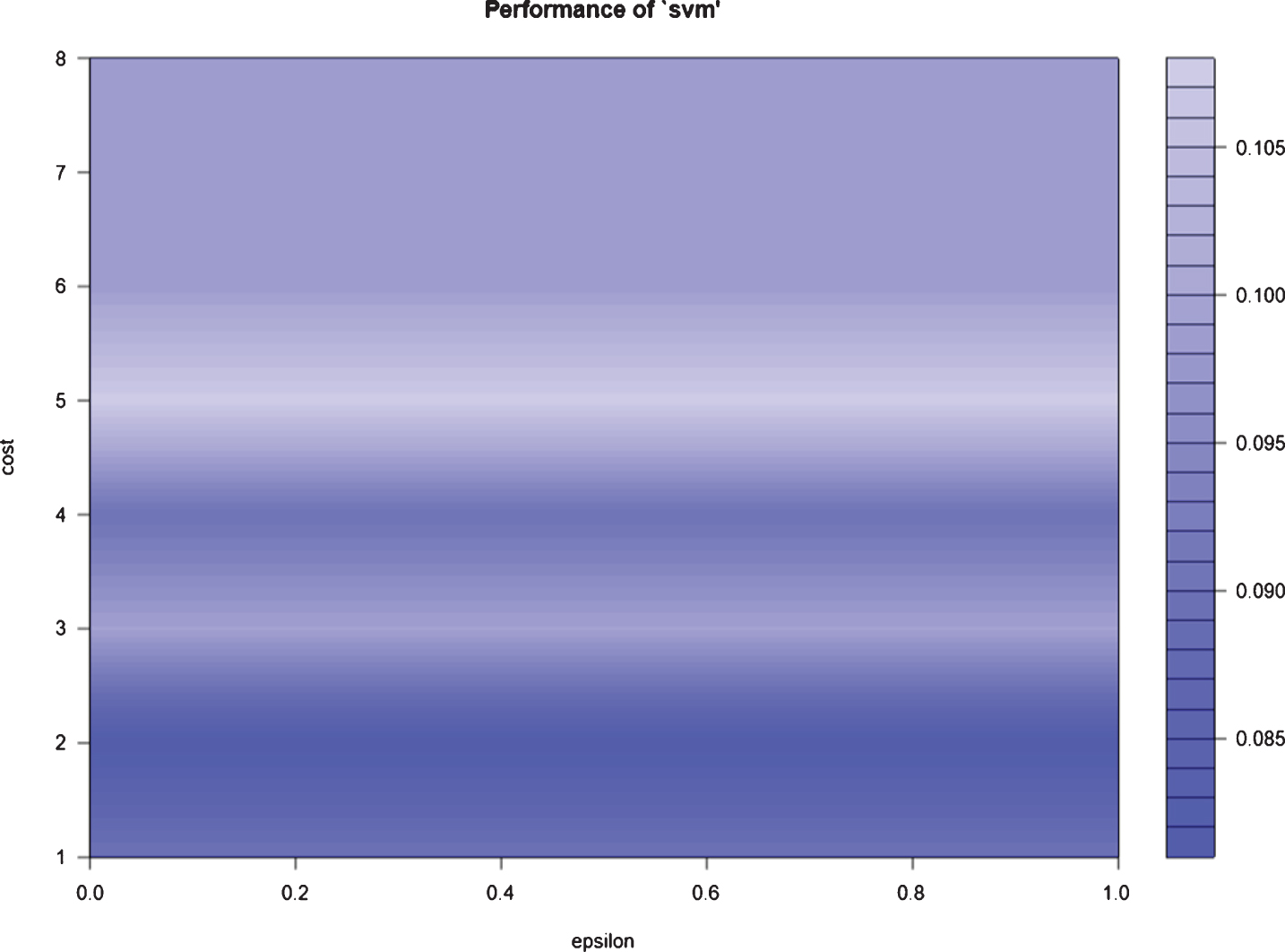
To find the appropriate kernel in our study, we have investigated four different kernels, namely linear kernel, radial base kernel (RBF), polynomial kernel, and sigmoid kernel. Based on the classification accuracy of both training and testing samples, we have decided to use the RBF kernel in our analysis. As shown in Fig. 3, the appropriate value of the cost (tuning parameter) is 2. In the training sample, out of the 62 bowlers, 3 were misclassified (Seekkuge Prasanna, Mohammad Saifuddin, and Imad Wasim). Out of the 50 batsmen in the training sample, 3 were misclassified (Moeen Ali, Dwayne Smith, and Moises Henriques). The model gave a correct classification rate of 94.64%, with an area under the curve 0.9458. In the testing sample, out of 21 bowlers, only Andre Russell was misclassified. Furthermore, out of the 16 batsmen, none were misclassified. The model predicted correctly 97.30% of the times, with an area under the ROC curve 0.9706. Fig. 8 shows the ROC curve for testing sample.
Fig. 3
Performance of SVM.
3.6Random forest
Random Forest (RF) is another machine learning technique that is applied to both classification and regression. As in the other approaches applied above, our goal here was to use it for classification. Random forest is a meta estimator consisting of a large number of individual decision trees on different subsamples of the training data, and it aggregates the outcomes of these decision trees to decide the class of the subjects. It applies the bootstrap aggregating method called bagging with model building. Bagging is a technique in which the algorithm collects a large number of uncorrelated trees to boost the predictive performance of the model. In random forest, the model is decided based on an error rate called out-of-bag (OOB) error, which is calculated using the left-out samples.
Tuning was done to control the training process and to gain better accuracy in model prediction. In random forest, tuning was focused on two parameters; the number of variables randomly selected to be sampled at each split, and the number of trees to grow to derive the average prediction. In our case, the number of variables randomly selected to be sampled at each split was 2 and the number of trees to grow for taking the average prediction was 300.
Application of random forest for classifying all-rounders resulted the following outcomes. In the training sample, out of the 62 bowlers and 50 batsman, none were misclassified. The correct classification rate was 100%, with an area under the curve 1. In the random forest, since the model used the data points many times during the resampling process, it is not uncommon to have a higher accuracy of prediction for the training sample. In the testing sample, out of the 21 bowlers only 1 was misclassified (Andre Russell). However, out of the 16 batsmen, 5 were misclassified (Corey Anderson, Dhananjaya de Silva, Grant Elliott, Kevin O’Brien, and Stuart Binny). The model gave a correct classification rate of 83.78%, with an area under the curve 0.9479 for the testing sample. Fig. 9 shows the ROC curve for testing sample.
4Discussion and conclusion
This paper focuses on utilizing the machine learning techniques to classify all-rounders in cricket. One can develop an automated classification rule based on the findings of this study, which can be used by cricket administrators with player selection. The remainder of this section summarizes the findings in detail.
Misclassified players based on different methods for the training and testing data sets are shown in Tables 4.1 and 4.2. Assessment of the performance of the methods were done using measures; accuracy and AUC. Fig. 4-9 give the ROC curves of the six classification techniques for testing data. Table 4.3 shows the accuracy of the methods separately for the training and testing samples. Table 4.4 gives the AUC values for the different classification methods. Evaluating the performance of different methods for testing sample is essential to assess the robustness of the models. Here, we start our discussion with the training sample and later conclude with the results for the testing sample.
Table 4.1
Misclassified Players in Training Data Set
| Name(bowling/batting)* | LR | LDA | QDA | NB | SVM | RF |
| Moeen Ali (batting) | NO | NO | YES | NO | YES | NO |
| Elton Chigumbura (batting) | NO | NO | NO | YES | NO | NO |
| James Faulkner (bowling) | NO | YES | NO | YES | NO | NO |
| Colin Grandhomme (batting) | NO | NO | YES | YES | NO | NO |
| Mominul Haque (batting) | YES | YES | YES | YES | NO | NO |
| Moises Henriques (batting) | YES | YES | YES | YES | YES | NO |
| Mosaddek Hossain (batting) | NO | NO | YES | NO | NO | NO |
| Nasir Hossain (batting) | NO | NO | YES | YES | NO | NO |
| Mohammad Nabi (battiing) | NO | NO | YES | NO | NO | NO |
| Hardik Pandya (batting) | YES | NO | YES | NO | NO | NO |
| Andile Phehlukwayo (bowling) | NO | YES | YES | NO | NO | NO |
| Seekkuge Prasanna (bowling) | NO | NO | YES | YES | YES | NO |
| Mohammad Saifuddin (bowling) | YES | YES | YES | YES | YES | NO |
| Dwayne Smith (batting) | YES | YES | YES | YES | YES | NO |
| Imad Wasim (bowling) | YES | YES | NO | YES | YES | NO |
* Original classification.
Table 4.2
Misclassified Players in Testing Data Set
| Names (bowling/batting)* | LR | LDA | QDA | NB | SVM | RF |
| Corey Anderson (batting) | YES | NO | NO | NO | NO | YES |
| Stuart Binny (batting) | YES | NO | NO | YES | NO | YES |
| Dhananjaya de Silva (batting) | NO | NO | YES | YES | NO | YES |
| Grant Elliott (batting) | NO | NO | NO | NO | NO | YES |
| Al-Amin Hossain (bowling) | NO | NO | NO | YES | NO | NO |
| Kevin O’Brien (batting) | NO | NO | NO | YES | NO | YES |
| Andre Russell (bowling) | NO | YES | NO | YES | YES | YES |
| Dasun Shanaka (batting) | YES | NO | NO | NO | NO | NO |
* Original classification.
Fig. 4
Logistics Regression.
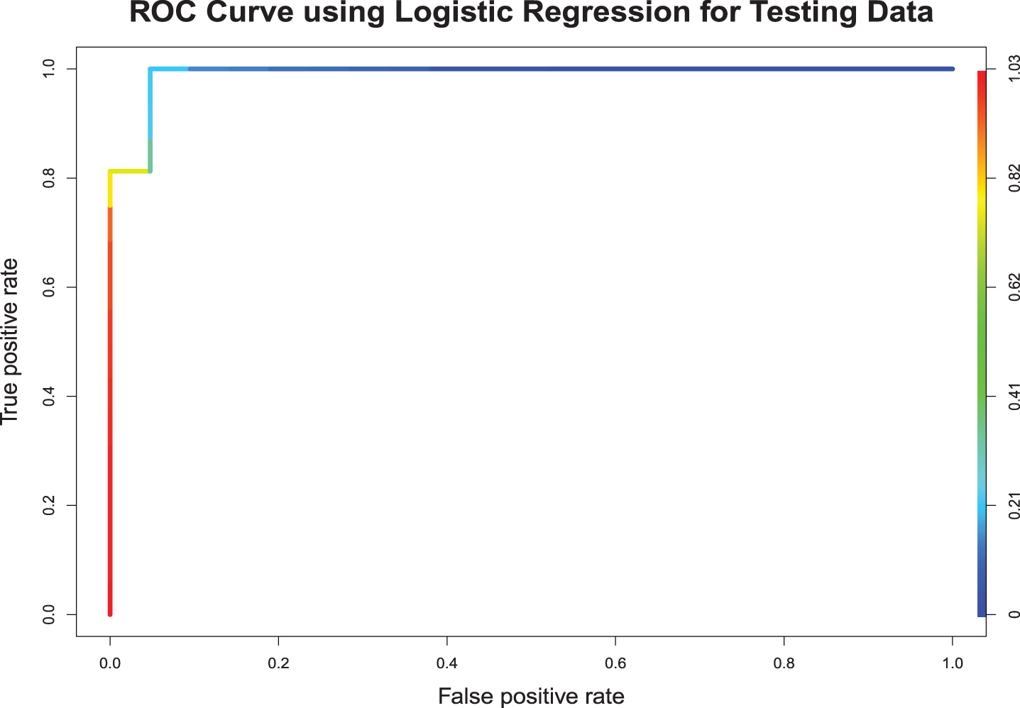
Fig. 5
Linear Discriminant Function.
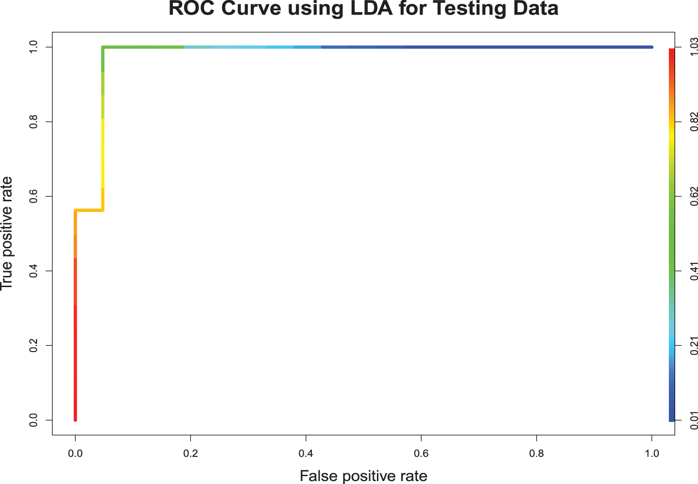
Fig. 6
Quadratic Discriminant Function.
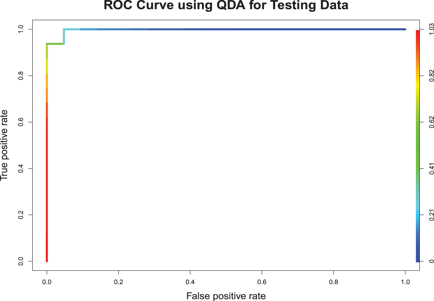
Fig. 7
Naíve Bayes.
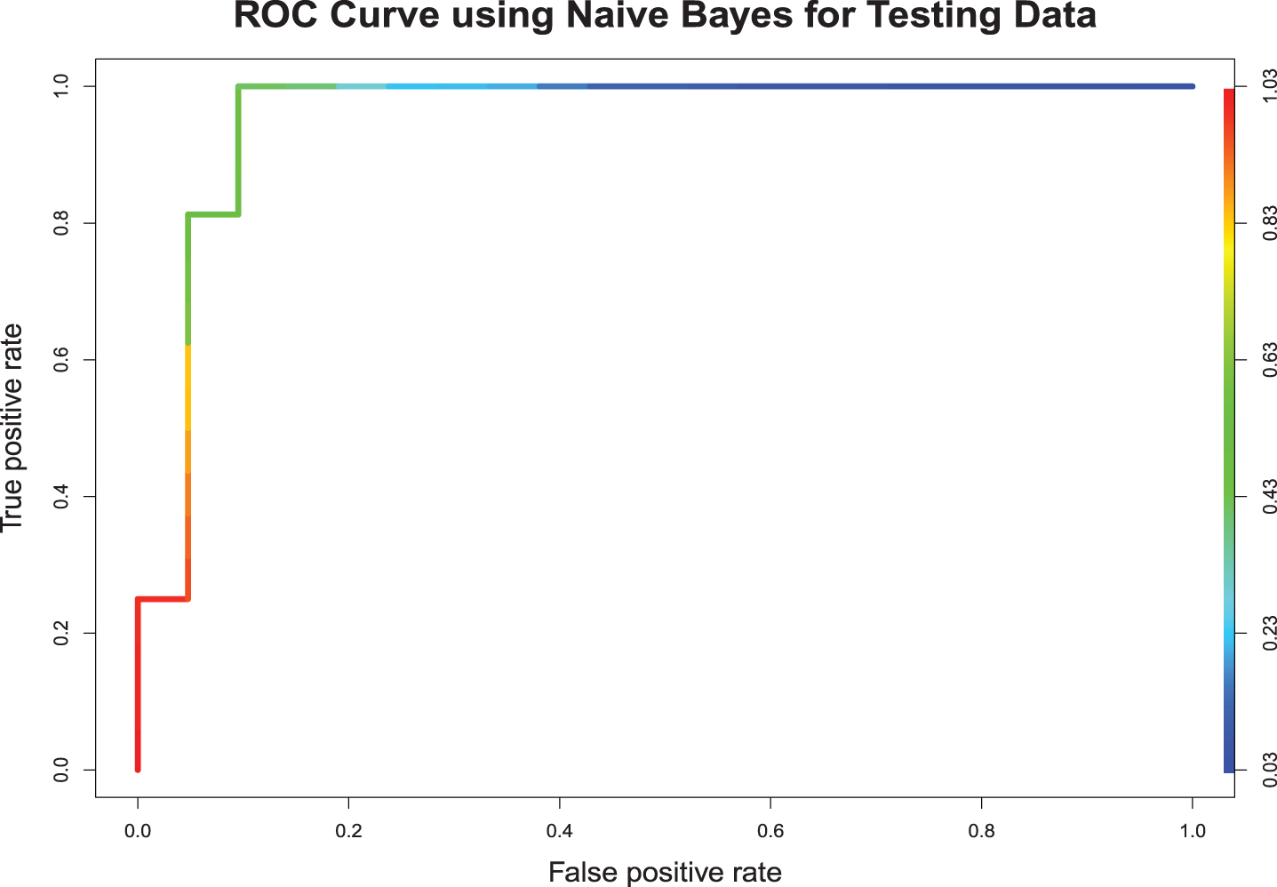
Fig. 8
Support Vector Machine.
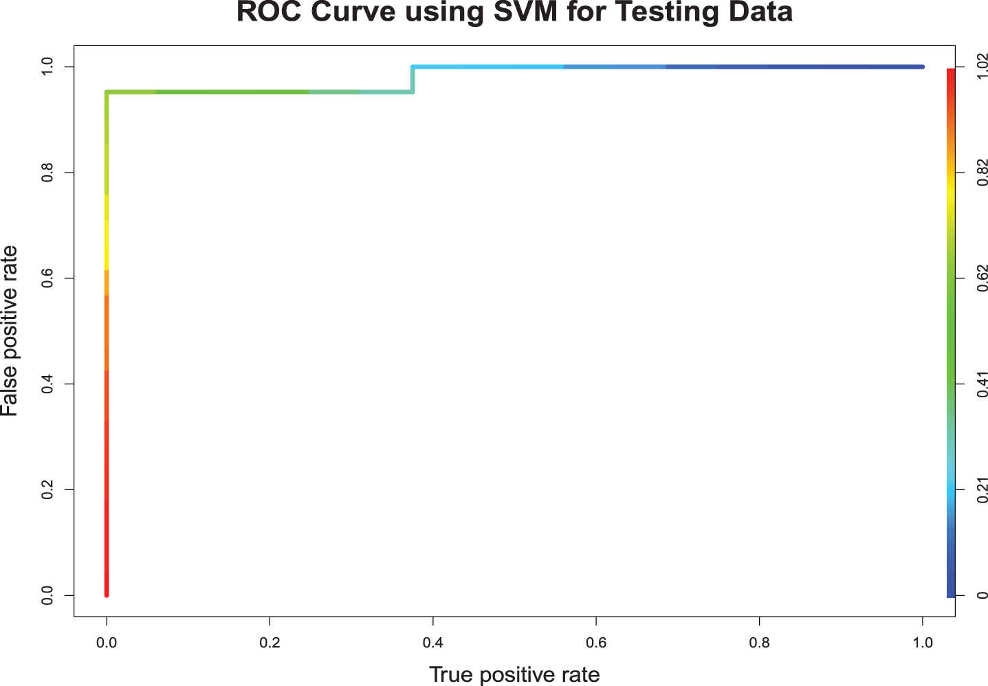
Fig. 9
Random Forest.
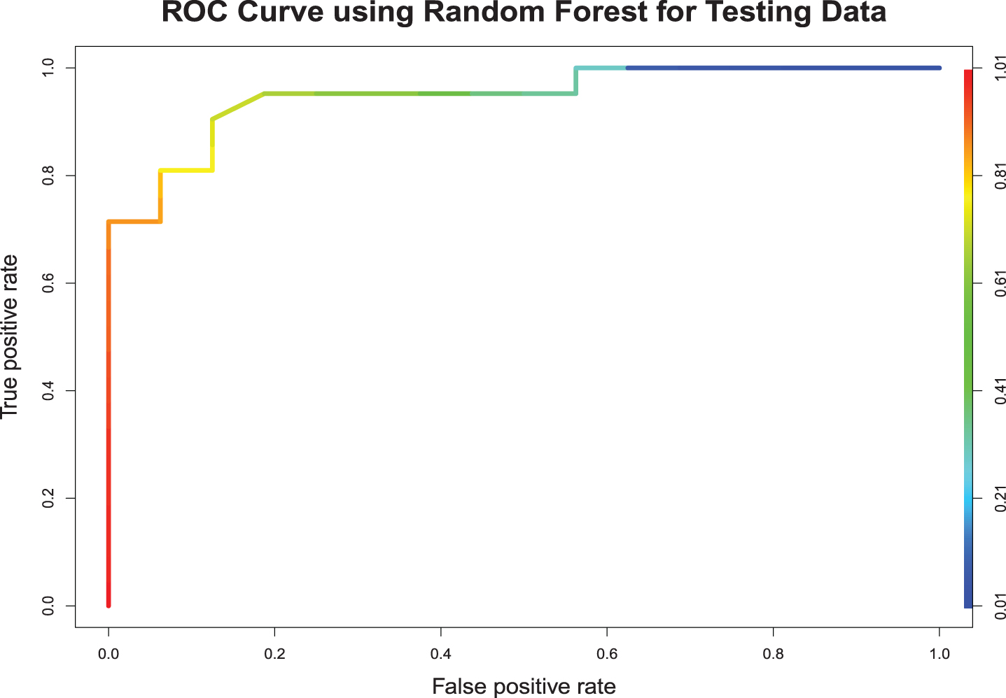
Table 4.3
Accuracy-Correct Classification
| Method | Training Data | Testing Data |
| LR | 0.9464 | 0.9189 |
| LDA | 0.9375 | 0.9730 |
| QDA | 0.8929 | 0.9730 |
| NB | 0.9107 | 0.8649 |
| SVM | 0.9464 | 0.9730 |
| RF | 1.0000 | 0.8378 |
Table 4.4
Area Under the ROC Curve
| Method | Training Data | Testing Data |
| LR | 0.9829 | 0.9912 |
| LDA | 0.9729 | 0.9792 |
| QDA | 0.9645 | 0.9970 |
| NB | 0.9716 | 0.9554 |
| SVM | 0.9458 | 0.9706 |
| RF | 1.0000 | 0.9479 |
For the training sample, random forest was the most accurate classification method, resulting in no misclassifications. However, as we discuss later, this method had serious overfitting issues. This is common for the random forest method due to the repeated resampling in the model building process. As we see from Table 4.4, AUC for all six methods is above 0.9458 (lowest, which was for SVM), which is an indication that these classifiers do an outstanding job in classifying all-rounders in the training sample. There were 3 players who were misclassified by all the methods except the random forest method. As we evaluate the classification methods, we scrutinized these players to see if there were any errors in the original classification. Those players were Mohammad Saifuddin, Dwayne Smith, and Moises Henriques.
Mohammad Saifuddin is a player from Bangladesh who was categorized as a bowling all-rounder in our original data set. He has played 20 innings with a bowling average of 37.87, which was somewhat higher than the mean for bowling all-rounders (32.45). This means that he concedes more runs per wicket than a typical bowling all-rounder. His bowling strike rate was 38.00, which was slightly lower than the mean for bowling all-rounders (38.35). This shows that he is slightly better than an average bowling all-rounder, in terms of number of balls used per wicket. His economy rate of 5.98 shows that he concedes more runs per over than even a typical batting all-rounder, where the mean economy rate for batting all-rounders was 5.94. He has a batting average of 29.11, which is closer to the mean for a batting all-rounder than that of a bowling all-rounder. His batting strike rate was 81.36, which was above the mean for bowling all-rounders (76.32) but below the mean for batting all-rounders (87.63). Considering these figures, one can argue that Mohammad Saifuddin is more of a batting all-rounder than a bowling all-rounder. Consequently, this could be the reason for him to be misclassified in five of the methods we considered. In hindsight, we think, he should have been classified as a batting all-rounder. This however, clearly affirms the reliability of the classification techniques we used.
Dwayne Smith is a West Indies cricketer who was categorized as a batting all-rounder in our original classification. He is an explosive batsman who can also break partnerships using effective bowling. He had comparable bowling statistics with a bowling average of 37.45, which was better than the mean for a typical batting all-rounder (48.78). He also had a bowling strike rate of 44.6, which was better than the mean of a batting all-rounder (53.03). His economy rate, 5.02, was better than even that of a typical bowling all-rounder. This shows that Dwayne Smith is a real all-rounder who can effectively contribute to the team in both batting and bowling. Five of our methods categorized him as a bowling all-rounder, contrary to our original categorization as a batting all-rounder. This also shows that the effectiveness of the classification technique that we used.
Moises Henriques is an Australian player who was categorized as a batting all-rounder in our original classification. His batting statistics were low in ODI cricket, but higher in Twenty20, which is the 20 over version of the limited over cricket format. That may have been the reason for him to be categorized as a batting all-rounder in our original list. However, our methods used statistics from the ODI matches, which evaluated him as an ODI all-rounder. That could be the reason why he was classified as a bowling all-rounder by five of our six methods.
Based on Tables 4.2 and 4.3, we see that for the testing sample, support vector machine, linear discriminant function, and quadratic discriminant function show significantly better performance than the other three methods. Each of these three methods misclassified only a single player giving a correct classification rate above 0.97. Logistic regression had an accuracy rate of 0.9189. Random forest and Naive Bayes method performed poorly relative to the other methods for the validation sample. As can be seen from the AUC values in Table 4.4, all six methods performed well for the testing sample which assures the robustness of the classification. Logistic regression, linear discriminant function, quadratic discriminant function, and support vector machine were all highly accurate, with AUC values 0.9912, 0.9792, and 0.9970, and 0.9706 respectively. Even the random forest and naive Bayes method that showed lower accuracy had considerably high AUC values (0.9479 and 0.9554 respectively). As a further investigation, we scrutinize three players who were missclassified by at least three methods we considered. These players were Andre Russell, Stuart Binny, and Dhananjaya Silva.
Andre Russell is a West Indies bowling all-rounder. He was misclassified by the linear discriminant analysis, naíve Bayes, support vector machine, and random forest methods in our analysis. In the international arena, he has played 47 innings to score 1034 runs, with a batting average of 27.21 and a batting strike rate of 130.22. In bowling, he has played 55 innings to take 70 wickets, with a bowling average 31.84, an economy rate 5.84, and batting strike rate 32.7. In the batting order, he has mostly played in positions 7, 8, and 9, with the median position 8. That justifies why he has been categorized as a bowling all-rounder in our original classification. However, as a batsman, his average was 27.21, which was closer to the mean batting average for batsmen (33.74), and his strike rate is 130.22, which is significantly higher than the mean strike rate for batsmen (87.63). Consequently, these classification methods suggest that Andre Russell should have been categorized as a batting all-rounder instead of a bowling all-rounder and we believe that should have been the correct classification for him. This also justifies the appropriateness and the effectiveness of the classification techniques authors suggesting for all-rounder classification in this article.
Stuart Binny is a batting all-rounder who had a short ODI career, with 11 innings of batting that accumulated 230 runs, with a batting average 28.75 and a batting strike rate of 93.49. His batting average was slightly below the mean batting average for batsmen (33.74), but his batting strike rate was well above the mean strike rate for batsmen (87.63). That could be the reason why he has been categorized as a batsman in our original classification. However, his bowling statistics indicate that he has also shown equally impressive performance as a bowler. He conceded considerably fewer runs per wicket (with a 21.95 bowling average) than a typical bowler (32.45). He also used far fewer balls per wicket (with a 24.5 bowling strike rate) than a typical bowler (38.35). His outstanding bowling performance may be the reason why he was misclassified as a bowler by logistics regression, naïve Bayes, and random forest methods.This further shows the preciseness of the classification techniques we used.
Dhananjaya de Silva is a Sri Lankan player who plays as a batting all-rounder for the national team. He has played 38 innings as a batsman and scored 796 runs in total for the period of this study. His batting average was 25.67, which was a bit lower than the average for a batsman (33.74). His batting strike rate was 75.02, which was also lower than that of a typical batsman (87.63). As a batsman, he has played in every position starting from the opening pair to the 9th position. His median position was 6, which may have been the reason for him to be categorized as a batting all-rounder in our original list. As a bowler, he has played 33 innings to accumulate 20 wickets. His bowling average was 40.55 and his strike rate was 45.4. Both of these figures were too high for an effective bowler. As we have seen, his batting figures were also not to the level of an effective batsman. Consequently, we can categorize him as an under-performer in both areas, batting and bowling. While he has been categorized as a batting all-rounder due to his front-order batting positions in our original classification, he has been misclassified by three of our classification methods, namely quadratic discriminant analysis, naíve Bayes, and random forest. Furthermore, based on his statistics, we believe that Dhananjaya Silva is yet to establish his position as a batting all-rounder or a bowling all-rounder. Misclassification of a such a player is not a weakness of a specific classification method.
This study has shown the capability of machine learning techniques for classifying all-rounders in cricket. Based on the findings of this study, it is clear that logistic regression, linear discriminant function, quadratic discriminant function, and support vector machine can be used to develop an automated classification rule that can be used by cricket administrators and team managers with player selection. A classification rule that incorporates all the above four methods would be highly effective. Furthermore, the sample size (number of matches) could play a significant role in classification accuracy. It will be an interesting future study to investigate the effect of the sample size on the classification accuracy of the methods that we discussed in this article.
Appendices
Appendix
Table A1
Confusion Matrices for Logistic Regression
| (A) Training Data | ||||
| Predicted | ||||
| bowl | bat | |||
| Actual | bowl | 60 | 02 | |
| bat | 04 | 46 | ||
| (B) Testing Data | ||||
| Predicted | ||||
| bowl | bat | |||
| Actual | bowl | 21 | 00 | |
| bat | 03 | 13 | ||
Table A2
Confusion Matrices for LDA
| (A) Training Data | ||||
| Predicted | ||||
| bowl | bat | |||
| Actual | bowl | 58 | 04 | |
| bat | 03 | 47 | ||
| (B) Testing Data | ||||
| Predicted | ||||
| bowl | bat | |||
| Actual | bowl | 58 | 04 | |
| bat | 03 | 47 | ||
Table A3
Confusion Matrices for QDA
| (A) Training Data | ||||
| Predicted | ||||
| bowl | bat | |||
| Actual | bowl | 58 | 04 | |
| bat | 08 | 42 | ||
| (B) Testing Data | ||||
| Predicted | ||||
| bowl | bat | |||
| Actual | bowl | 21 | 00 | |
| bat | 01 | 15 | ||
Table A4
Confusion Matrices for Naíve Bayes
| (A) Training Data | ||||
| Predicted | ||||
| bowl | bat | |||
| Actual | bowl | 58 | 04 | |
| bat | 06 | 44 | ||
| (B) Testing Data | ||||
| Predicted | ||||
| bowl | bat | |||
| Actual | bowl | 19 | 02 | |
| bat | 03 | 13 | ||
Table A5
Confusion Matrices for SVM
| (A) Training Data | ||||
| Predicted | ||||
| bowl | bat | |||
| Actual | bowl | 59 | 03 | |
| bat | 03 | 47 | ||
| (B) Testing Data | ||||
| Predicted | ||||
| bowl | bat | |||
| Actual | bowl | 20 | 01 | |
| bat | 01 | 15 | ||
Table A6
Confusion Matrices for Random Forest
| (A) Training Data | ||||
| Predicted | ||||
| bowl | bat | |||
| Actual | bowl | 62 | 00 | |
| bat | 00 | 50 | ||
| (B) Testing Data | ||||
| Predicted | ||||
| bowl | bat | |||
| Actual | bowl | 20 | 01 | |
| bat | 05 | 11 | ||
References
1 | Agarwal, S. , Yadav, L. and Mehta, S. (2017) , Cricket Team Prediction with Hadoop: Statistical Modeling Approach, Procedia Computer Science, 122: , 525–532. |
2 | Akhtar, S. and Scarf, P. (2012) , Forecasting test cricket match outcomes in play, International Journal of Forecasting, 28: (3), 632–643. |
3 | Asif, M. and McHale, I. G. (2016) , In-play forecasting of win probability in One-Day International cricket: A dynamic logistic regression model, International Journal of Forecasting, 32: (1), 34–43. |
4 | Baboota, R. and Kaur, H. (2019) , Predictive analysis and modelling football results using machine learning approach for English Premier League, International Journal of Forecasting, 35: (2), 741–755. |
5 | Bunker, R. P. and Thabtah, F. (2019) , A machine learning framework for sport result prediction, Applied Computing and Informatics, 15: (1), 27–33. |
6 | Cust, E. E. , Sweeting, A. J. , Ball, K. and Robertson, S. (2019) , Machine and deep learning for sport-specific movement recognition: a systematic review of model development and performance, Journal of Sports Sciences, 37: (5), 568–600. |
7 | Davis, J. , Perera, H. and Swartz, T. B. (2015) , Player evaluation in Twenty20 cricket, Journal of Sports Analytics, 1: (1), 19–31. |
8 | James, G. , Witten, D. , Hastie, T. and Tibshirani, R. (2013) ) An Introduction to Statistical Learning with Application in R, Springer. |
9 | Jayalath, K. P. (2018) , A machine learning approach to analyze ODI cricket predictors, Journal of Sports Analytics, 4: (1), 73âĂŞ84. |
10 | Jayanth, S. B. , Anthony, A. , Abhilasha, G. , Shaik, N. and Srinivasa, G. (2018) , A team recommendation system and outcome prediction for the game of cricket, Journal of Sports Analytics, 4: (4), 263–273. |
11 | Khan, J. R. , Biswas, R. K. and Kabir, E. (2019) , A quantitative approach to influential factors in One Day International cricket: Analysis based on Bangladesh, Journal of Sports Analytics, 5: (1), 57–63. |
12 | Leung, C. K. and Joseph, K. W. (2014) , Sports data mining: predicting results for the college football games, Procedia Computer Science, 35: , 710–719. |
13 | Manage, A. B. , Scariano, S. M. (2013) , An Introductory Application of Principal Components to Cricket Data, Journal of Statistics Education, 21: (3). |
14 | Ofoghi, B. , Zeleznikow, J. , Dwyer, D. and Macmahon, C. (2013) , Modelling and analysing track cycling Omnium performances using statistical and machine learning techniques, Journal of Sports Sciences, 31: (9), 954–962. |
15 | Pathak, N. and Wadhwa, H. (2016) , Applications of modern classification techniques to predict the outcome of ODI Cricket, Procedia Computer Science, 87: , 55–60. |
16 | Rein, R. , Memmert, D. (2016) ) Big data and tactical analysis in elite soccer: future challenges and opportunities for sports science., SpringerPlus 5(1). |
17 | Saikia, H. and Bhattacharjee, D. (2011) , On Classification of All-rounders of the Indian Premier League (IPL): A BaYESian Approach, Vikalpa, 36: (4), 51–66. |
18 | Thabtah, F. , Zhang, L. and Abdelhamid, N. (2019) , NBA game result prediction using feature analysis and machine learning, Ann Data Sci, 6: (1), 103âĂŞ116. |
19 | Wickramasinghe, I. (2020) , Naive Bayes approach to predict the winner of an ODI cricket game, Journal of Sports Analytics, 6: (2), 75âĂŞ84. |
20 | Yi, J. and Wang, X.Q. (2019) , Study on safety mode of dragon boat sports physical fitness training based on machine learning, Safety Science, 120: , 1–5. |


