
On the relationship between +/– ratings and event-level performance statistics
Abstract
This work considers the challenge of identifying and properly assessing the contribution of a single player towards the performance of a team. In particular, we study the use of advanced plus-minus ratings for individual football players, which involves evaluating a player based on the goals scored and conceded with the player appearing on the pitch, while compensating for the quality of the opponents and the teammates as well as other factors. To increase the understanding of plus-minus ratings, event-based data from matches are first used to explain the observed variance of ratings, and then to improve their ability to predict outcomes of football matches. It is found that event-level performance statistics can explain from 22% to 38% of the variance in plus-minus ratings, depending on player positions, while incorporating the event-level statistics only marginally improves the predictive power of plus-minus ratings.
1Introduction
The development of ratings for individual players in team sports has attracted increased attention from researchers in recent years, as the availability and quality of data have improved. Such individual ratings are not straightforward to derive, but potentially offer valuable inputs to fans (McHale et al., 2012), media (Tiedemann et al., 2011), clubs (Macdonald, 2012), coaches (Schultze and Wellbrock, 2018), associations (Hass and Craig, 2018), tournament organizers (McHale et al., 2012), gamblers and bookmakers (Engelmann, 2017), and the players themselves (Tiedemann et al., 2011).
This paper contributes to the understanding of a particular type of rating system, collectively known as plus-minus (PM) ratings. PM ratings have been developed for basketball players (Engelmann, 2017), ice-hockey players (Gramacy et al., 2017), volleyball players (Hass and Craig, 2018), and association football players (Sæbø and Hvattum, 2019). For additional historical references and a discussion of key publications on PM ratings, the reader can consult a recently published review paper (Hvattum, 2019). While simpler forms of PM ratings exist, the focus in this paper is on (regularized) adjusted PM ratings, calculated using some form of (regularized) regression model.
A particular feature of PM ratings is that they only use information about how the score changes during matches and about which players appear on the playing field at different points in time. This contrasts to methods that apply detailed event-based data to derive player ratings, typically focusing on particular aspects of play, such as goal scoring or passing (Szczepański, 2015).
Arguments against the top-down perspective of PM ratings include that it is unreasonable to distribute credit of performance onto players without knowing the actual actions taken by players. However, bottom-up ratings that depend on the actions taken by players typically also miss some aspects of play that the top-down perspective could capture, such as the motivating influence on teammates. In addition, unless tracking-data is available, bottom-up ratings would have to ignore typical off-the-ball actions that may be important in many team sports.
The purpose of this work is to increase our understanding about the relationship between PM ratings and event-based performance statistics of individual players in association football. This relationship has not previously been examined in football, but there is some related work from basketball.
Rosenbaum (2004, 2005) examined adjusted PM ratings for basketball. He also calculated a set of game statistics, measured per 40 minutes of playing time. The adjusted PM ratings were regressed on the game statistics, to estimate how different actions can explain the players’ PM ratings. Using in total 14 independent variables, including pure and derived game statistics, the multiple linear regression model could explain 44% of the variance in the PM rating. Furthermore, the regression coefficients were used to directly calculate a statistical PM rating, which turned out to provide ratings with smaller standard errors, and which in turn could be combined with the initial PM ratings for yet another rating measure.
Fearnhead and Taylor (2011) used a Bayesian framework to calculate adjusted PM ratings, where each player received both an offensive and a defensive rating. Regressing the PM ratings on ten different dependent variables, they were able to explain 41% of the variance of the offensive ratings, but only 3% of the variance of the defensive ratings.
There are few papers comparing the quality of PM ratings and alternative ratings. Engelmann (2011) developed an ad hoc player rating for basketball players that made use of information about individual player actions. The ad hoc model was better at predicting point differentials than a regularized PM rating. Matano et al. (2018) compared regularized PM ratings for football with ratings from the FIFA computer game series, which are partly based on subjective inputs from scouts. They showed that the PM ratings outperformed the FIFA ratings in two out of three seasons. By using the FIFA ratings as priors for the PM ratings, the resulting ratings outperformed the other two ratings in all three seasons.
Given the context of using PM ratings to evaluate individual players in football, the goal of this paper is three-fold. One goal is to test whether PM ratings capture the information contained in event-level player performance statistics. The second goal is to test the extent to which past event-level statistics contain information that is not captured by PM ratings and that can be used to improve predictions for outcomes of future football matches. The third goal is to test whether improved player ratings can be derived by combining the PM ratings with information from player events.
The remainder of the paper is structured as follows. Section 2 provides information about the data used, the calculation of the plus-minus ratings that are analyzed, and the variables derived from event data. Results from regressing PM ratings on the performance statistics are presented in Section 3. Section 4 contains results from tests using PM ratings and performance statistics to predict match outcomes. The attempts at deriving improved player ratings are discussed in Section 5, and Section 6 concludes the paper.
2Experimental setup
The data consist of individual on-the-ball player events recorded for the seasons 2009–2017 in five European Tier 1 domestic competitions (English Premier League, French Ligue 1, German Bundesliga, Italian Serie A and Spanish La Liga). Cartesian pitch coordinates are given for each event, and passes are encoded with origin and end-point coordinates. Four matches were incomplete and excluded from the analysis, leaving 16,430 matches in the analysis dataset. There were approximately 1,514 on-the-ball events per match. In addition to the on-the-ball player events, the data contain information about substitutions and players sent off, so that at any time the players present on the pitch are known.
2.1Plus-minus ratings
The PM ratings that we analyze in this work are based on a model presented by Pantuso and Hvattum (2019), which is an extension of the work by Sæbø and Hvattum (2015, 2019). The model is formulated as an unconstrained quadratic program, which generalizes a multiple linear regression model estimated using ridge regression (Tikhonov regularization).
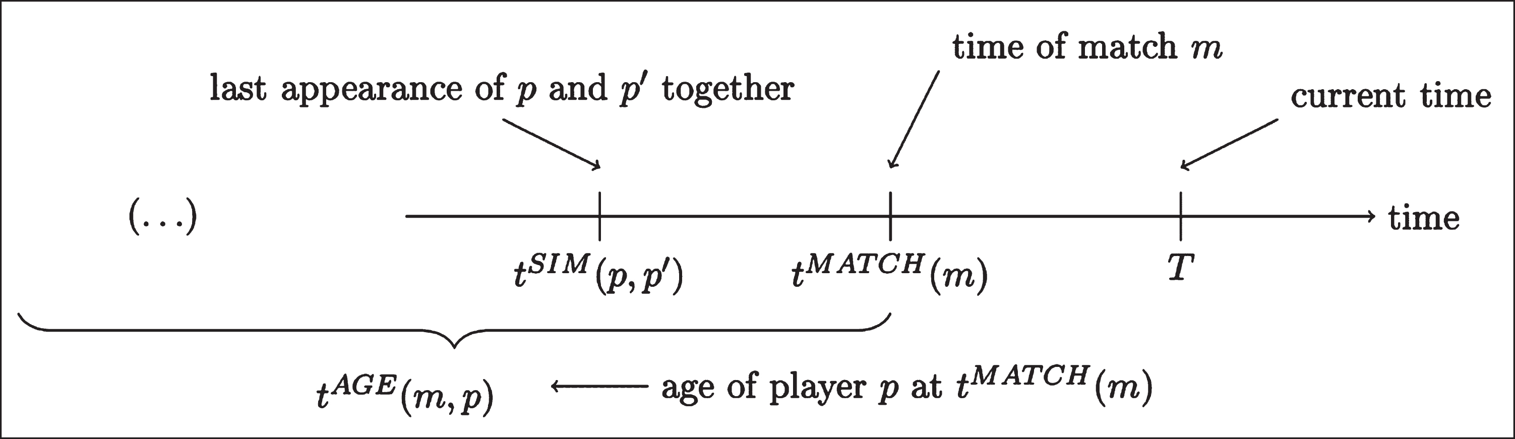
Let M be a set of matches, where each match m ∈ M is split into a set of segments Sm. For our PM ratings this is done by creating one segment for each interval with no changes to the players appearing on the pitch. In other words, segments are created for each substitution and each red card. The duration of segment s ∈ Sm is denoted by d (m, s). Let t = tMATCH (m) denote the time that match m is played, and let T be the current time, at which ratings are calculated. The parameters of the model associated to the timing of events are illustrated in Fig. 1. Each match belongs to a given competition type, such as the English Premier League, or the Spanish La Liga. Denote the competition type of match m by c (m).
Fig. 1
Illustration of the parameters referring to the time of events.
Let h = h (m) and a = a (m) be the two teams involved in match m, where h is the home team, unless the match is played on neutral ground. The goal difference in favour of h in segment s ∈ Sm of match m is denoted by g (m, s). We also define g0 (m, s) as the goal difference in favour of h at the beginning of the segment, and g1 (m, s) as the goal difference at the end of the segment.
The set of players of team t∈ { h, a } that appear on the pitch for segment s is denoted by Pm,s,t. For n = 1, . . . , 4, define r (m, s, n) = 1 if team h has received n red cards and team a has not, r (m, s, n) = -1 if team a has received n red cards and team h has not, and r (m, s, n) = 0 otherwise. We let C be the set of competition types and define Cp as the set of competition types in which player p has participated. Each player p is associated to a set
The model includes an age profile, as the playing strength of players is expected to improve while young and then decline when getting older. To this end, tAGE (m, p) is defined as the age of player p at the time of match m. A discrete set of possible age values Y ={ yMIN, …, yMAX } is defined, and for a given match and player, the age of the player is taken as a convex combination of the possible age values. That is, by introducing parameters u (y, tMATCH (m) , p) to select among the age combinations, it holds that max { min { tAGE (m, p) , yMAX } , yMIN } = ∑y∈Yu (y, tMATCH (m) , p) y, where at most two values u (y, tMATCH (m) , p) are non-zero, ∑y∈Yu (y, tMATCH (m) , p) = 1, and 0 ≤ u (y, tMATCH (m) , p) ≤1. As an example, tMATCH (m) = 25.4 would result in the unique combination of u (25, tMATCH (m) , p) = 0.6, u (26, tMATCH (m) , p) = 0.4, and u (y, tMATCH (m) , p) =0. for y∉ { 25, 26 }.
Define the following parameters: λ is a regularization factor, ρ1 is a discount factor for older observations, ρ2 and ρ3 are parameters regarding the importance of the duration of a segment, and ρ4 is a factor for the importance of a segment depending on the goal difference at the start of the segment. The parameter wAGE is a weight to balance the importance of the age factors when considering similarity of players. Finally, wSIM is a weight that controls the extent to which ratings of players with few minutes played are shrunk towards 0 or towards the ratings of similar players. The values of the parameters are set as in (Pantuso and Hvattum, 2019).
The variables used in the model can be stated as follows. Let βp correspond to the base rating of player p. The value of the home advantage in competition c (m) is represented by
The full model for our PM ratings can now be written as follows:
This is a way to express the estimation of a multiple linear regression model with Tikhonov regularization. In particular, w (m, s) fLHS (m, s) corresponds to the values of the independent variables, w (m, s) fRHS (m, s) represents the value of the dependent variable, and fREG (βj) expresses the regularization penalties. The rating model defined here generalizes this by allowing fREG (βj) to deviate from the standard regularization terms.
Defining the details of the rating model, w (m, s) is a weight that is used to express the importance of a given segment s of match m:
The dependent variable is simply the observed goal difference from the perspective of the home team, multiplied by the weight of the observation:
The independent variables can be split into those that describe properties of each player, fPLAYER (m, s, p), those that describe properties of a given segment fSEGMENT (m, s), and those that describe a given match, fMATCH (m). These are defined as follows:
Finally, the form of fREG (βj) varies for the different regression coefficients. For the competition adjustment coefficients,
The estimated rating for player p at time T can now be written as fAUX (p, T, 1). For large data sets, solving the unconstrained quadratic programming can become time consuming. Sæbø and Hvattum (2015) described how a simpler version of the ratings can be estimated using commercially available software. However, in this model, regularization terms for the player ratings fREG (βp) and for the age effects
The calculations outlined above provides a point estimate for the rating of each player. To provide a measure of the uncertainty in the rating of each player, we sugge to use bootstrapping (Fox, 2008, Chapter 21). In this procedure, observations from a regression model are sampled with replacement, until the bootstrap sample has the same size as the original data set. The model is then estimated on the bootstrap sample and the relevant values are recorded, which in our case means recording fAUX (p, T, 1) for each player p. By repeating the bootstrap procedure multiple times, confidence intervals for the rating of a given player can be derived by referring to the percentiles of the recorded ratings for that player.
2.2Variables
Key performance indicators (KPIs) are derived for each player from counts of the associated ball-touch events. In Table 1, definitions are provided of the different events that are counted. Then, Table 2 gives the definitions for how the KPIs are derived from the event counts.
Table 1
Definitions of counted events
| Counted Event | Definition |
| Aerial Duel | When two players contest a 50/50 ball in the air, each player is awarded an aerial duel. The winning player is awarded a successful aerial duel and the losing player is awarded an unsuccessful duel. |
| Assist | A pass to a teammate who scores a goal. |
| Block | An interception where the intercepting player is close to the passing player |
| Card | Referee issues a yellow (warning) card or a red card. A player issued a red card is sent off the pitch for the rest of the game. |
| Clearance | A player under pressure kicks the ball clear of the defensive zone or out of play. |
| Dispossessed | Player is tackled and loses possession of the ball. |
| Foul Attracted | The player is fouled according to the referee, and is awarded a free kick. |
| Foul Committed | The referee judges a player to have committed a foul. |
| Goal | All goals, including penalty goals. |
| Ground Duel | A ground duel event is counted for both players involved in a tackle or take on event. The winning player is awarded a successful ground duel and the losing player is awarded an unsuccessful duel. |
| Interception | Player intercepts a pass and prevents it reaching its intended destination. |
| Key Pass | A pass to a teammate who makes an unsuccessful attempt on goal. |
| Loose Ball Recovered | Player takes possession of a loose ball when both teams have lost possession. |
| Pass | Pass from one player towards a teammate. Passes from dead-ball situations such as throw-ins, free-kicks, goal-kicks and corner kicks are included. A pass is successful if it reaches a teammate or unsuccessful if it is intercepted or goes out of play. |
| Save (Goalkeeper) | Goalkeeper saves a shot on goal. |
| Save (Outfield player) | Player blocks a shot on goal. |
| Shot on Target | An attempt on goal that is on target (includes goals). |
| Tackle Made | Player dispossess an opponent of the ball. |
| Take-On | Player attempts to dribble ball past an opponent. A successful take on is awarded if the player dribbles past. |
| Through Ball | A pass made for an attacker to run on to and create a goal attempt. |
| Touch | Any touch of the ball. |
Table 2
Definitions of key performance indicators
| Key Performance Indicator | Definition |
| .../90 | Per 90 event count. Event count divided by the number of minutes played and multiplied by 90 to give a per 90 statistic. |
| % Aerial Duels Won | Count of successful aerial duels as a percentage of total aerial duels. |
| % Ground Duels Won | Count of successful ground duels as a percentage of total ground duels. |
| % Passes Completed | Count of Successful passes as a percentage of total passes. |
| Mean Pass Length | Total Pass Length/Total number of passes. |
| Pass Value | Pass value is calculated by an algorithm which awards positive values to successful passes that move the ball incrementally closer to the opposition goal and penalizes unsuccessful passes that concede position close to player’s own goal. |
| Saves-to-Shots Ratio | Goalkeepers only. Count of saves divided by count of saves plus goals conceded. |
| Times Dispossessed per Touch | Count of dispossessions divided by count of touches. |
| Total Pass Length | Sum of lengths of successful passes (m.) |
3Regressing ratings on key performance indicators
For this phase of the analysis we use matches in the seasons 2009–2016. Because per 90 KPIs are unstable when a player has played only a few minutes, players with fewer than 540 minutes playing time (equivalent to six full-time matches) are excluded. Twenty-four KPIs that are commonly used to evaluate players are entered into the analysis. One KPI (Saves-to-Shots Ratio) is only defined for goalkeepers. The correlations of the KPIs with PM ratings are reported in Table 3. Statistical significance levels are indicated by *** for p <0.001, ** for p <0.01, and * for p <0.05.
Table 3
Correlations of KPIs with PM ratings
| KPI | r |
| Touches/90 | 0.35*** |
| Successful Passes/90 | 0.34*** |
| Saves-to-Shots Ratio† | 0.30*** |
| % Passes Completed | 0.27*** |
| Successful Take-Ons/90 | 0.25*** |
| Total Pass Length/90 | 0.24*** |
| Assists/90 | 0.23*** |
| Key Passes/90 | 0.22*** |
| Goals Scored/90 | 0.18*** |
| Shots on Target/90 | 0.16*** |
| Loose Balls Recovered/90 | 0.15*** |
| Clearances/90 | –0.12*** |
| Saves/90 | –0.09*** |
| Cards/90 [neg] | 0.09*** |
| Fouls Committed/90 [neg] | 0.09*** |
| Through Balls/90 | 0.07*** |
| Pass Value/90 | 0.07*** |
| Interceptions &Blocks/90 | 0.07*** |
| % Ground Duels Won | 0.06*** |
| % Aerial Duels Won | –0.03 |
| Mean Pass Length | 0.03 |
| Tackles Made/90 | 0.02 |
| Times Dispossessed per Touch [neg] | 0.01 |
| Successful Aerial Duels/90 | 0.00 |
Note: † = Goalkeepers only, N = 395, otherwise outfield players only, N = 4,726.
Most of the KPIs correlate positively with PM ratings, indicating some convergence between the two measures of player quality. This is further explored by a series of ordinary least squares regression analyses below. Separate regression equations were estimated for each player position, and in each case, the predictors were selected by a filtering process (Saeys, Inza, & Larrañaga, 2007). The data was resampled according to a five-fold cross-validation scheme, and a generalized additive model was used to screen for a significant relationship between the plus-minus ratings and a spline on each of the candidate predictors (23 KPIs for outfield players, 24 for goalkeepers). The procedure was repeated three times, producing 15 cross-validation samples. Table 4 reports statistics for the R2 values obtained.
Table 4
Variances explained statistics in 15 cross-validation samples
| Position | Mean R2 | SD R2 | Minimum R2 | Maximum R2 |
| Goalkeepers | 21.7% | 9.3% | 7.7% | 40.2% |
| Defenders | 36.2% | 3.8% | 31.1% | 44.6% |
| Defensive Midfielders | 27.0% | 6.9% | 15.7% | 41.8% |
| Midfielders | 33.3% | 6.6% | 23.6% | 45.0% |
| Attacking Midfielders | 33.5% | 10.0% | 15.2% | 47.7% |
| Forwards | 36.1% | 7.1% | 25.7% | 52.7% |
Predictors that survived this filtering process were used in the positional regression equations reported below. Residuals in each positional equation were tested for normality and heteroscedasticity and outlying/influential observations removed (Peña & Slate, 2006). After removal of these observations (only necessary for defenders and midfielders), all tests for heteroscedasticity and departures from skewness and kurtosis were non-significant at p ≤ 0.05, indicating that the linear model assumptions of normality and constant variance were satisfied.
Tables 5 to 10 show the regression models for the full positional datasets. Table 11 shows the relative importance of the predictors for each position.
Table 5
KPIs to explain PM of goalkeepers, explains 22.4% of variance
| estimate | std. error | statistic | |
| (Intercept) | –0.330 | 0.063 | –5.23*** |
| % Passes Completed | 0.271 | 0.060 | 4.50*** |
| Saves-to-Shots Ratio | 0.249 | 0.053 | 4.67*** |
| % Ground Duels Won | 0.013 | 0.010 | 1.35 |
| Successful Aerial Duels/90 | 0.069 | 0.021 | 3.30** |
| Pass Value/90 | –0.010 | 0.012 | –0.86 |
| F = 22.4, df = (5, 389) |
Note: N = 395.
Table 6
KPIs to explain PM of defenders, explains 36.1% of variance
| estimate | std. error | statistic | |
| (Intercept) | –0.088 | 0.029 | –3.00*** |
| Successful Passes/90 | 0.003 | 0.000 | 14.07*** |
| Successful Aerial Duels/90 | 0.016 | 0.002 | 9.77*** |
| Key Passes/90 | 0.029 | 0.005 | 5.76*** |
| Pass Value/90 | 0.026 | 0.005 | 5.45*** |
| Successful Take-Ons/90 | 0.014 | 0.003 | 4.54*** |
| Interceptions &Blocks/90 | 0.007 | 0.002 | 4.51*** |
| Fouls Committed/90 [neg] | 0.005 | 0.003 | 1.52 |
| Goals Scored/90 | 0.022 | 0.028 | 0.79 |
| Saves/90 | 0.004 | 0.006 | 0.75 |
| Assists/90 | 0.031 | 0.033 | 0.94 |
| Cards/90 [neg] | 0.003 | 0.011 | 0.31 |
| % Passes Completed | 0.000 | 0.039 | 0.01 |
| F = 88.61, df = (12, 1802) |
Note: N = 1,815.
Table 7
KPIs to explain PM of defensive midfielders, explains 30.7% of variance
| estimate | std. error | statistic | |
| (Intercept) | –0.156 | 0.037 | –4.19*** |
| Successful Passes/90 | 0.002 | 0.000 | 5.11*** |
| Successful Take-Ons/90 | 0.028 | 0.005 | 5.08*** |
| Interceptions &Blocks/90 | 0.014 | 0.004 | 3.13** |
| % Ground Duels Won | 0.062 | 0.048 | 1.28 |
| % Passes Completed | 0.052 | 0.061 | 0.86 |
| Tackles Made/90 | 0.000 | 0.005 | –0.08 |
| F = 20.86, df = (6, 283) |
Note: N = 290.
Table 8
KPIs to explain PM of midfielders, explains 35.0% of variance
| estimate | std. error | statistic | |
| (Intercept) | –0.247 | 0.021 | –11.53*** |
| Touches/90 | 0.001 | 0.000 | 5.27*** |
| Successful Take-Ons/90 | 0.018 | 0.003 | 6.94*** |
| % Passes Completed | 0.217 | 0.029 | 7.63*** |
| Goals Scored/90 | 0.074 | 0.019 | 3.84*** |
| Key Passes/90 | 0.022 | 0.004 | 5.48*** |
| Interceptions &Blocks/90 | 0.010 | 0.002 | 4.46*** |
| Assists/90 | 0.065 | 0.027 | 2.4* |
| Times Dispossessed per Touch [neg] | 0.179 | 0.142 | 1.26 |
| Through Balls/90 | –0.002 | 0.007 | –0.35 |
| Fouls Committed/90 [neg] | 0.003 | 0.003 | 0.93 |
| Tackles Made/90 | 0.000 | 0.002 | –0.2 |
| Saves/90 | 0.013 | 0.010 | 1.34 |
| F = 48.73, df = (12, 1084) |
Note: N = 1,097.
Table 9
KPIs to explain PM of attacking midfielders, explains 36.4% of variance
| estimate | std. error | statistic | |
| (Intercept) | –0.126 | 0.037 | –3.39*** |
| Key Passes/90 | 0.025 | 0.005 | 5.44*** |
| Successful Take-Ons/90 | 0.019 | 0.003 | 7.29*** |
| Goals Scored/90 | 0.063 | 0.022 | 2.82*** |
| % Passes Completed | 0.103 | 0.051 | 2.05* |
| Assists/90 | 0.055 | 0.032 | 1.75 |
| Fouls Committed/90 [neg] | 0.003 | 0.004 | 0.75 |
| Successful Aerial Duels/90 | 0.003 | 0.003 | 1.18 |
| Pass Value/90 | 0.012 | 0.006 | 1.96 |
| Successful Passes/90 | 0.001 | 0.000 | 2.87** |
| Cards/90 [neg] | 0.015 | 0.019 | 0.82 |
| Clearances/90 | 0.015 | 0.005 | 2.77** |
| F = 28.78, df = (11, 553) |
Note: N = 565.
Table 10
KPIs to explain PM of forwards, explains 37.9% of variance
| estimate | std. error | statistic | |
| (Intercept) | –0.155 | 0.027 | –5.82*** |
| Shots on Target/90 | 0.012 | 0.005 | 2.49* |
| Successful Take-Ons/90 | 0.012 | 0.003 | 4.49*** |
| Goals Scored/90 | 0.087 | 0.014 | 6.36*** |
| Key Passes/90 | 0.024 | 0.004 | 6.14*** |
| Interceptions &Blocks/90 | 0.018 | 0.004 | 4.94*** |
| % Passes Completed | 0.129 | 0.033 | 3.95*** |
| Assists/90 | 0.099 | 0.025 | 4.05*** |
| Pass Value/90 | 0.015 | 0.004 | 3.62*** |
| Successful Aerial Duels/90 | 0.005 | 0.002 | 3.00** |
| Cards/90 [neg] | 0.022 | 0.014 | 1.53 |
| % Ground Duels Won | 0.046 | 0.034 | 1.37 |
| F = 49.45, df = (11, 890) |
Note: N = 902.
Table 11
Relative importance of KPIs by position
| KPI | GK | D | DM | M | AM | FW |
| Successful Aerial Duels/90 | 11.9% | 10.0% | 0.0% | 0.0% | ||
| Assists/90 | 2.2% | 6.8% | 11.6% | 9.4% | ||
| Clearance/90 | 0.0% | |||||
| Cards/90 [neg] | 0.6% | 1.8% | 0.9% | |||
| Fouls Committed/90 [neg] | 0.8% | 0.9% | 1.9% | |||
| Saves-to-Shots Ratio | 28.6% | |||||
| Goals Scored/90 | 0.9% | 4.8% | 8.3% | 22.4% | ||
| Interceptions &Blocks/90 | 3.1% | 10.6% | 7.2% | 3.4% | ||
| Key Passes/90 | 10.3% | 10.3% | 26.2% | 22.3% | ||
| Times Dispossessed per Touch [neg] | 1.3% | 0.4% | ||||
| Successful Passes/90 | 50.6% | 47.4% | 13.9% | |||
| % Ground Duels Won | 3.6% | 3.3% | 4.1% | |||
| % Passes Completed | 48.2% | 13.1% | 13.7% | 20.5% | 8.0% | 6.7% |
| Pass Value/90 | 7.7% | 3.2% | 2.6% | 3.4% | ||
| Saves/90 | 0.2% | 0.1% | ||||
| Shots on Target/90 | 14.2% | |||||
| Tackles Made/90 | 3.7% | 0.5% | ||||
| Successful Take-Ons/90 | 4.9% | 21.3% | 16.3% | 25.7% | 12.8% | |
| Through Balls/90 | 1.1% | |||||
| Touches/90 | 30.4% |
Tables 5 through 10 show that player PM ratings are related to a wide variety of KPIs which are conditional upon player position, and suggest that PM ratings capture a range of positionally relevant skills.
Table 11 shows the relative importance (CAR scores; Zuber and Strimmer, 2011) of the KPIs in each regression equation, and the values in each column sum to 100%. So for example, the value of 8.4% for Successful Aerial Duels/90 in the defenders column means that this KPI contributes 8.4% of the explained variance in PM ratings for defenders, while the value of 1.8% for Assists/90 means that this KPI contributes a much smaller proportion, and is accordingly a less important predictor of PM ratings.
The overall pattern of results seems plausible. For instance, the most important predictors of PM ratings for forwards are Goals Scored/90, Key Passes/90 and Shots on Target/90. For attacking midfielders, the most important predictors are Key Passes/90, Successful Take-Ons/90, and Successful Passes/90. For the other outfield positions, Goals, Key Passes and Shots are less important, and Successful Passes/90 and % Passes Completed dominate the other predictors of PM ratings. For midfielders the dominant predictor is Touches/90, but if this KPI is forced out of the regression equation, it is replaced by Successful Passes/90 as the most dominant predictor.
The shared variance between KPIs and PM ratings indicates a modest degree of convergent validity (Campbell and Fiske, 1959) between the top-down and bottom-up metrics of evaluating players. Nevertheless, it is clear that most of the variance in PM ratings cannot be explained by the bottom-up indicators we have examined here.
4Predicting match outcomes using ratings and key performance indicators
PM ratings can be used as a basis for predicting outcomes of football matches where the starting line-ups are known (Sæbø and Hvattum, 2019), by using the difference of the average ratings of home team players and away team players as a single covariate in an ordered logit regression (OLR) model (Greene, 2012). In this section we test whether information from KPIs can be used as additional covariates to improve the prediction quality.
To this end, seasons 2009 through 2015 are used to calculate initial values for PM ratings and KPIs for each player. Seasons 2016 and 2017 provide initial observations for the OLR, where player ratings and KPIs are updated before each new day with matches played. Finally, season 2017 is used as the validation set: before each day of matches, player ratings and KPIs are updated and the regression model is re-estimated using all current information. Then, the predictions are generated for each match of the day, and the quadratic loss (Witten et al., 2011) of the prediction is calculated.
Five models are considered. Model 1 has only one covariate, based on the PM ratings of the players in the starting line-up. Model 2 has 32 covariates, one based on PM ratings, and the rest derived from KPIs. The KPIs included are the 24 from Table 1, in addition to Aerial Duels Won/90, Aerial Duels Lost/90, Unsuccessful Passes/90, Unsuccessful Take-Ons/90, Challenges/90, Saves by Goalkeeper/90, and Fouls Attracted/90. For the KPI-based covariates, the values are first calculated for each individual player in the starting line-up, and then the covariate is calculated as the difference between the averages for the two teams.
To improve the second model, a form of recursive feature elimination (Guyon et al., 2002) is used. The feature selection is performed before considering the data in the validation set and is based on recursively eliminating the covariate that leads to the greatest improvement in the Bayesian information criterion (BIC) until no covariates are left. The final set of covariates retained is the set that provided the best value of BIC throughout the procedure. Starting from Model 2 and performing such feature selection results in Model 3. Models 4 and 5 are created in the same manner as Model 2 and Model 3, respectively, but without including the PM ratings as one of the initial covariates.
Table 12 presents, for each model, the log-likelihood when estimating the model on the full data set, the quadratic loss from out-of-sample predictions in the validation set, and the final regression coefficients. Model 2 and Model 4 are omitted from the table. Their log-likelihood measures are –5112.2 and –5157.6, respectively, while their quadratic loss, which is more importantly addressing their out-of-sample performance, is 0.5684 and 0.5731. Despite their performance thus being slightly better than that of Model 3 and Model 5, we prefer to focus our further analysis on the more parsimonious models. The main reason for this is that the regression coefficients in Model 2 and Model 4 are largely not statistically significant.
Table 12
Ordered logit estimation of three different models. Log-likelihoods and regression coefficients are reported for models using observations from seasons 2015 to 2017. Quadratic loss is calculated out-of-sample for season 2017. Standard errors are reported in parentheses. All the reported coefficients have significance levels of p <0.001
| Model 1 | Model 3 | Model 5 | |
| Log-likelihood | –5161.0 | –5141.1 | –5193.1 |
| Quadratic loss | 0.5704 | 0.5689 | 0.5770 |
| θ1. | –0.197 (0.029) | –0.206 (0.029) | –0.206 (0.029) |
| θ2 | 1.015 (0.033) | 1.014 (0.033) | 0.995 (0.033) |
| PM Rating | –1.215 (0.042) | –0.998 (0.056) | |
| Successful Passes/90 | –0.045 (0.005) | ||
| Clearance/90 | –0.289 (0.069) | ||
| Loose Balls Recovered/90 | –0.235 (0.055) | ||
| Saves/90 | 0.967 (0.225) | 1.718 (0.254) | |
| Key Passes/90 | –0.559 (0.133) | –1.093 (0.137) | |
| Goals Scored/90 | –3.477 (0.625) | ||
| Saves-to-Shots Ratio | –1.096 (0.233) |
The models without PM ratings are worse at predicting future matches, with a higher quadratic loss. On the other hand, Model 3, which adds covariates based on the number of saves and the number of key passes to the model with only PM ratings, is able to predict future matches slightly better. For comparison, a model with no covariates, thus predicting future matches based on past frequencies of outcomes only, obtains a quadratic loss of 0.6442, and a log-likelihood value of –5668.1.
This indicates that the PM ratings do not fully incorporate useful information derived from looking at the number of saves and the number of key passes during a match. As the regression coefficient of Saves/90 is positive, it means that a higher number of saves is associated with worse future results. An increased number of key passes, on the other hand, is associated with higher probabilities of better results. In total, 24 different KPIs were included in Model 2 and Model 4, but were removed by the feature selection for both Model 3 and Model 5
5Improving ratings using key performance indicators
In this section, we discuss two attempts at creating improved PM ratings for individual football players. The first attempt is based on the regression results in Section 3, where the PM ratings were regressed on player KPIs. Rosenbaum (2004, 2005) did this for basketball players, and then suggested a statistical PM rating, where the rating of each player is calculated directly from the regression formulas obtained and the observed KPIs. As a next step, a convex combination of the statistical PM and the regular PM was calculated so as to minimize an error measure.
Rosenbaum (2004, 2005) proposed the statistical PM and its combination with regular PM ratings mainly to reduce the noise in the ratings. This work was performed on adjusted PM, before the use of regularization was popularized (Sill, 2010). As noise is a much less significant issue in the PM ratings used here, the combination of statistical PM and regular PM ratings may be less effective. A difference to the statistical PM ratings of Rosenbaum (2004, 2005), is that our regressions are performed for each player position separately.
To calibrate the overall rating, as a convex combination of statistical PM and regular PM, we consider the log-likelihood of an OLR model fitted on observed match results in the training data, with a single covariate based on the overall rating. The relative weight of statistical PM is varied in a grid search from 0 to 1 in intervals of 0.05. Figure 2 shows the obtained log-likelihoods. The best log-likelihood is obtained for a weight equal to 0.05, which means that there is some value in the statistical PM, but not much. For comparison, in (Rosenbaum, 2005), a weight of 0.4 was used for the statistical PM.
Fig. 2
Tuning of the overall rating combining statistical PM and regular PM.
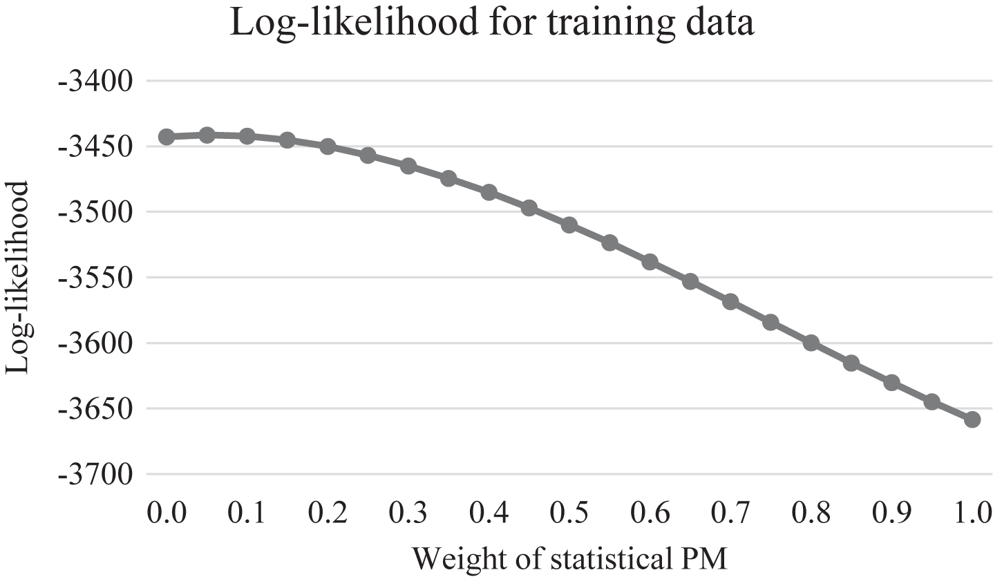
Table 12 shows the results of Model 6, which uses the combined rating as the basis of a single co-variate to predict future matches. Comparing with the results of Model 1 in Table 12, we can see that the new rating performs only slightly better. Furthermore, Table 14 and Table 15 show the top 20 rated players according to PM ratings and the new combined rating, calculated based on the whole data set. The top-rated players are mostly identical for the two ratings, which is as expected, given that a weight of 0.95 is used on the regular PM ratings in the combined rating.
Table 13
Ordered logit estimation of two additional models. Values reported as in Table 12. All the reported coefficients have significance levels of p <0.001
| Model 6 | Model 7 | |
| Log-likelihood | –5148.4 | –5141.0 |
| Quadratic loss | 0.5701 | 0.5688 |
| θ1 | –0.199 (0.029) | –0.206 (0.029) |
| θ2 | 1.016 (0.033) | 1.013 (0.033) |
| PM + Statistical Rating | –1.254 (0.044) | |
| Enhanced PM Rating | –1.448 (0.050) |
Table 14
Top 20 players according to the regular PM rating. Also shown are results from the bootstrapping procedure, showing the median bootstrap rating as well as the limits of a 90 % confidence interval for the estimated rating. All ratings calculated based on data from seasons 2009 through 2017
| Bootstrapped ratings | Diff. to Muller | |||||||
| Name | Position | Rating | Minutes | 5 % | Median | 95 % | 5 % | 95 % |
| Thomas Muller | FW | 0.278 | 21531 | 0.233 | 0.273 | 0.310 | NA | NA |
| Lionel Messi | FW | 0.269 | 25297 | 0.221 | 0.262 | 0.301 | –0.042 | 0.070 |
| T. Alcantara | M | 0.266 | 10207 | 0.214 | 0.258 | 0.301 | –0.032 | 0.067 |
| Neymar | FW | 0.260 | 11947 | 0.202 | 0.253 | 0.300 | –0.038 | 0.080 |
| David Alaba | D | 0.257 | 16080 | 0.215 | 0.250 | 0.291 | –0.019 | 0.065 |
| Ederson | GK | 0.257 | 3263 | 0.198 | 0.248 | 0.292 | –0.036 | 0.086 |
| Toni Kroos | M | 0.255 | 20767 | 0.205 | 0.247 | 0.287 | –0.025 | 0.079 |
| Danilo | D | 0.249 | 4694 | 0.188 | 0.237 | 0.293 | –0.032 | 0.096 |
| Marcelo | D | 0.240 | 20820 | 0.194 | 0.235 | 0.274 | –0.013 | 0.090 |
| Casemiro | M | 0.238 | 6077 | 0.188 | 0.228 | 0.265 | –0.011 | 0.099 |
| R. Lewandowski | FW | 0.237 | 20165 | 0.188 | 0.228 | 0.271 | 0.003 | 0.087 |
| Jerome Boateng | D | 0.237 | 16084 | 0.193 | 0.231 | 0.274 | –0.002 | 0.085 |
| Mohamed Salah | FW | 0.228 | 9543 | 0.179 | 0.219 | 0.265 | –0.007 | 0.108 |
| James Rodriguez | M | 0.224 | 9377 | 0.171 | 0.218 | 0.261 | 0.001 | 0.108 |
| Nacho F. | D | 0.223 | 7232 | 0.176 | 0.215 | 0.261 | 0.001 | 0.108 |
| Kyle A. Walker | D | 0.218 | 20286 | 0.158 | 0.209 | 0.254 | 0.004 | 0.120 |
| Mario Gotze | AM | 0.215 | 13305 | 0.166 | 0.209 | 0.253 | 0.007 | 0.122 |
| Marco Verratti | M | 0.215 | 11185 | 0.169 | 0.203 | 0.241 | 0.013 | 0.119 |
| Pedro | FW | 0.214 | 17301 | 0.161 | 0.207 | 0.253 | 0.006 | 0.122 |
| Raphael Varane | D | 0.213 | 13136 | 0.168 | 0.210 | 0.249 | 0.013 | 0.118 |
Table 15
Top 20 players according to the combined rating using statistical PM and regular PM, and the new enhanced PM based on PM in combination with saves and key passes. All ratings calculated based on data from seasons 2009 through 2017. For enhanced PM, only players with more than 540 minutes of playing time are included
| Statistical + Regular PM | Enhanced PM | ||||
| Thomas Muller | FW | 0.270 | Lionel Messi | FW | 0.313 |
| Lionel Messi | FW | 0.268 | Neymar | FW | 0.310 |
| T. Alcantara | M | 0.262 | Thomas Muller | FW | 0.304 |
| Neymar | FW | 0.258 | R. Lewandowski | FW | 0.300 |
| David Alaba | D | 0.252 | C. Ronaldo | FW | 0.269 |
| Ederson | GK | 0.249 | J. Rodriguez | M | 0.259 |
| Toni Kroos | M | 0.249 | Toni Kroos | M | 0.256 |
| Danilo | D | 0.243 | Luis Suarez | FW | 0.255 |
| Marcelo | D | 0.234 | Mohamed Salah | FW | 0.251 |
| R. Lewandowski | FW | 0.233 | Arjen Robben | AM | 0.248 |
| Jerome Boateng | D | 0.232 | Kevin de Bruyne | AM | 0.248 |
| Casemiro | M | 0.230 | Mario Gotze | AM | 0.247 |
| Mohamed Salah | FW | 0.224 | Karim Benzema | FW | 0.244 |
| James Rodriguez | M | 0.221 | Angel di Maria | FW | 0.237 |
| Nacho F. | D | 0.217 | Franck Ribery | AM | 0.236 |
| Kyle A. Walker | D | 0.212 | T. Alcantara | M | 0.234 |
| Marco Verratti | M | 0.212 | Mesut Ozil | AM | 0.229 |
| Mario Gotze | AM | 0.211 | David Silva | AM | 0.228 |
| David Silva | AM | 0.208 | M. Mandzukic | FW | 0.227 |
| Pedro | FW | 0.208 | Sadio Mane | FW | 0.222 |
To evaluate the uncertainty of the rating estimates, Table 14 provides PM ratings based on 500 bootstrap samples (Fox, 2008). For the bootstrapped ratings, the median rating is shown together with the 5th and the 95th percentile ratings, thus providing a 90 % confidence interval for the PM rating. Additionally, we show a 90 % confidence interval for the difference in rating to Thomas Muller, the player with the highest PM rating. The latter is useful when determining whether a given player has a rating that is significantly different from the rating of another player, although only as a descriptive statistic of the players’ performances in the data set.
A second attempt at finding an improved rating is based on the regression results in Section 4. The results of Model 3 presented there, suggested that information about saves and key passes could be helpful to improve the regular PM ratings. To this end, we define an enhanced PM rating by taking a linear combination of the regular PM rating and the individual values for Saves/90 and Key passes/90 for each player. The weights of the linear combination are determined by maximizing the log-likelihood for an OLR model on the training data. A variant of coordinate search (Kolda et al., 2003; Schwefel, 1995) is used as a direct search method to optimize the log-likelihood as a function of the weights of the components in the enhanced PM rating. Starting the search with weights (1.0, 0.0, 0.0), the best weights found are (0.681, –0.0643, 0.0363), with a log-likelihood of –3427.87, which is slightly better than what was obtained using the combination of statistical PM and regular PM ratings.
Table 13 provides results for Model 7, using the enhanced PM rating as the basis for the sole covariate included in OLR to predict future match results. This model performs slightly better than the other models with only a single rating covariate, and even marginally better than Model 3. This confirms that information about saves and key passes can be used to improve the predictive ability of PM ratings.
However, it is also worthwhile to look at Table 14, showing the top 20 ranked players according to the enhanced PM ratings. For the enhanced PM ratings, it was necessary to enforce a cut-off based on the number of minutes played to produce the top 20 list. Whereas the regular PM ratings ensure that players with few minutes played are not represented in the extremes of the rating lists, this is not the case for enhanced PM ratings. Some players with few minutes recorded may obtain very high values for Key Passes/90, and thus will dominate the other players on the list.
When listing only players with more than 540 minutes of playing time, the top 20 list looks very reasonable, and perhaps even more so than the list based on regular PM ratings. However, while the top list for PM ratings contain players of all positions, the enhanced PM ratings seem to favour offensive players, and there are no goalkeepers and no defenders in the top 20.
6Discussion
Our first main finding is that top-down and bottom-up performance indicators for football players share a non-trivial amount of variance. For goalkeepers, regression of KPIs on PM ratings finds an R2 of 0.22, while for outfield players the R2 values range from 0.31 for defensive midfielders to 0.38 for forwards. These findings are comparable to previous research on NBA player ratings. Rosenbaum (2004, 2005) regressed PM ratings on fourteen different KPIs, reporting an R2 of 0.44. Fearnhead and Taylor (2011) regressed offensive and defensive PM ratings on a common set of ten KPIs, finding R2 values of 0.42 and 0.03 respectively.
Although these results show that some of the variance of PM ratings for football players can be explained by event data, most of the variance remains unexplained. It may be that some of the variance is due to properties not covered by the event data, such as a player’s ability to create or cover space, pressing that does not lead to ball interaction, and physical abilities such as pace. However, it may also be that a substantial part of the variance is simply noise, as was the case in early versions of PM ratings (Hvattum, 2019).
Our second main finding is that marginal improvements in the prediction of match results can be achieved by combining information from player top-down and bottom-up ratings. However, the application of multiple rating perspectives produces comparatively little change in the predicted probabilities of match results. Correlations between the modelled probabilities of a home win for the pure (Model 1), statistical (Model 6) and enhanced PM models (Model 7) are all over 0.98, as are the correlations between away win probabilities, while the correlations between draw probabilities are all over 0.97.
As the improvement in prediction quality for the versions of PM ratings incorporating event-based data is modest, it may be argued that the PM ratings, aggregated on a team level, provides a reasonable assessment of team quality. However, on a player level, the new enhanced PM rating has some interesting differences to the standard PM rating; while the two methods evaluate players within a given player position similarly, the different player positions are ranked differently. Within position correlations between the standard and enhanced ratings are uniformly high, ranging from 0.85 for goalkeepers to 0.94 for forwards. However, taken over all players, the correlation is 0.61.
For standard PM ratings and the mix of standard and statistical PM ratings, the average ranks for each player position are similar, as shown in Table 16. On the other hand, the enhanced PM rating suggests that forwards are the most influential, followed by attacking midfielders, whereas defenders and goalkeepers are less influential and receive lower ratings.
Table 16
Average rank for players of different positions, considering 5,499 players with at least 540 minutes of playing time, and three different PM ratings
| GK | D | DM | M | AM | FW | |
| PM | 2891.6 | 2793.8 | 2758.3 | 2771.6 | 2607.6 | 2656.9 |
| Statistical + Regular PM | 2893.6 | 2794.9 | 2761.5 | 2774.0 | 2604.4 | 2651.7 |
| Enhanced PM | 5252.4 | 3292.3 | 2862.7 | 2488.8 | 1696.9 | 1483.8 |
As two opposing teams will use a similar number of players from each position at any time, this shift in relative evaluation of players of different positions does not in itself lead to significant differences in predictions. For example, since all teams will almost always use exactly one goalkeeper, any shift in ratings of goalkeepers will not have any consequences for predictions made. Therefore, although enhanced PM has slightly better predictive power than the other two variants, it would be premature to conclude that goalkeepers and defenders are less important for winning football matches.
Combining different base learners often leads to reductions in noise and improvements in predictive accuracy (see e.g. Hanson and Salamon, 1990). A natural extension to the present research would therefore be to investigate a stacked ensemble that combines match predictions from a model based on PM ratings alone and a model based only on player KPIs.
References
1 | Campbell,D.T. and Fiske,D.W. , (1959) , Convergent and discriminant validation by the multitrait-multimethod matrix, Psychological Bulletin 56: , 81–105. |
2 | Engelmann,J. , (2011) , A new player evaluation technique for players of the National Basketball Association (NBA), Proceedings of the MIT Sloan Sports Analytics Conference. |
3 | Engelmann,J. , (2017) , Possession-based player performance analysis in basketball (adjusted +/- and related concepts). In J. Albert, M. Glickman, T. Swartz, and R. Koning, editors., Handbook of Statistical Methods and Analyses in Sports, pages 215-228. Chapman and Hall/CRC, Boca Raton. |
4 | Fearnhead,P. and Taylor,B. , (2011) , On estimating the ability of NBA players. Journal of Quantitative Analysis in Sports 7: , https://doi.org/10.2202/1559-0410.1298. |
5 | Fox,J. , (2008) , Applied Regression Analysis and Generalized Linear Models, Sage Publications, California, USA, 2nd edition. |
6 | Gramacy,R. , Taddy,M. and Tian,S. , (2017) , Hockey performance via regularized logistic regression. In J. Albert, M. Glickman, T. Swartz, and R. Koning, editors., Handbook of Statistical Methods and Analyses in Sports, pages 287-306. Chapman and Hall/CRC, Boca Raton. |
7 | Greene,W. , (2012) , Econometric Analysis. Pearson, Harlow, England, 7th edition. |
8 | Guyon,I. , Weston,J. , Barnhill,S. and Vapnik,V. , (2002) , Gene selection for cancer classification using support vector machines, Machine Learning 46: , 389–422. |
9 | Hansen,L.K. and Salamon,P. , (1990) , Neural network ensembles, IEEE Transactions on Pattern Analysis and Machine Intelligence 12: , 993–1001. |
10 | Hass,Z. and Craig,B. , (2018) , Exploring the potential of the plus/minus in NCAA women’s volleyball via the recovery of court presence information, Journal of Sports Analytics 4: , 285–295. |
11 | Hvattum,L.M. , (2019) , A comprehensive review of plus-minus ratings for evaluating individual players in team sports, International Journal of Computer Science in Sport 18: , 1–23. |
12 | Kolda,T.G. , Lewis,R.M. and Torczon,V.J. , (2003) , Optimization by direct search: New perspectives on some classical and modern methods, SIAM Review 45: , 385–482. |
13 | Macdonald,B. , (2012) , Adjusted plus-minus for NHL players using ridge regression with goals, shots, Fenwick, and Corsi, Journal of Quantitative Analysis in Sports 8: . |
14 | Matano,F. , Richardson,L. , Pospisil,T. , Eubanks,C. and Qin,J. , (2018) , Augmenting adjusted plus-minus in soccer with FIFA ratings, ArXiv:1810.08032v1. |
15 | McHale,I. , Scarf,P. and Folker,D. , (2012) , On the development of a soccer player performance rating system for the English Premier League, Interfaces 42: , 339–351. |
16 | Pantuso,G. and Hvattum,L.M. , (2019) , Maximizing performance with an eye on the finances: A chance constrained model for football transfer market decisions, ArXiv: 1911.04689v1. |
17 | Peña, E.A. , Slate,E.H. , ((2006) ). Global validation of linear model assumptions. Journal of the American Statistical Association 101: (473), 341–354. |
18 | Rosenbaum,D. , (2004) , Measuring how NBA players help their teams win, http://www.82games.com/comm30.htm, Accessed 2018-08-31. |
19 | Rosenbaum,D. , (2005) , Defense is all about keeping the other team from scoring, http://82games.com/rosenbaum3.htm, Accessed 2018-09-28. |
20 | Saeys, Y , Inza, I. , Larrañaga,P. , ((2007) ). A review of feature selection techniques in bioinformatics, Bioinformatics 23: , 2507–2517. |
21 | Schultze,S. and Wellbrock,C. , (2018) , A weighted plus/minus metric for individual soccer player performance, Journal of Sports Analytics 4: , 121–131. |
22 | Schwefel,H.P. , (1995) , Evolution and Optimum Seeking. Wiley-Interscience. |
23 | Sill,J. , (2010) , Improved NBA adjusted +/- using regularization and out-of-sample testing, Proceedings of the 2010 MIT Sloan Sports Analytics Conference. |
24 | Szczepański,Ł. , (2015) , Assessing the skill of football players using statistical methods. PhD thesis, University of Salford. |
25 | Sæbø,O.D. and Hvattum,L.M. , (2015) , Evaluating the efficiency of the association football transfer market using regression based player ratings. In NIK: Norsk Informatikkonferanse, 12 pages. Bibsys Open Journal Systems. |
26 | Sæbø,O.D. and Hvattum,L.M. , (2019) , Modelling the financial contribution of soccer players to their clubs, Journal of Sports Analytics 5: , 23–34. |
27 | Tiedemann,T. , Francksen,T. and Latacz-Lohmann,U. , (2011) , Assessing the performance of German Bundesliga football players: A non-parametric metafrontier approach, Central European Journal of Operations Research 19: , 571–587. |
28 | Witten,I. , Frank,E. and Hall,M.A. , (2011) , Data Mining: Practical Machine Learning Tools and Techniques. Morgan Kaufmann Publishers, 3rd edition. |
29 | Zuber,V. and Strimmer,K. , (2011) , High-dimensional regression and variable selection using CAR scores, Statistical Applications in Genetics and Molecular Biology 10. |


