
Dynamically scheduling NFL games to reduce strength of schedule variability
Abstract
The National Football League (NFL) schedules regular season games so that some matchups are based on the previous year’s results. Since team composition changes from year to year, this scheduling policy creates variation in teams’ strength of schedules and sometimes benefits teams unfairly, allowing some an easier path to the playoffs than others. This paper proposes methods to produce an NFL schedule that combine some of its traditional elements with dynamically scheduled games aimed at optimizing different objectives, such as reducing the variability of teams’ strength of schedule or minimizing the number of pairwise comparisons needed to differentiate team quality so as to make each teams’ regular season schedule as fair as possible.
1Introduction
Many sports leagues, college and professional, have tournaments or playoffs at the end of the season to crown a champion. Ideally, to determine which teams should make the playoffs, each team would play every other team in a round-robin fashion so that each team would have an equalized strength of schedule. However, in sports where few games are played, such as football, or where there are many more teams than available games, such as college basketball and baseball, the possibility of creating a round-robin season schedule is unrealistic. So, without head-to-head information, the problem of choosing which teams should make the playoffs creates debate about which factors are most important in that selection.
Two important factors often mentioned in these debates are a team’s strength of schedule and head-to-head results (pairwise comparisons). Strength of schedule is often an important consideration, especially when a team with a mediocre record played a particularly tough schedule or when an undefeated team played a weaker schedule. Traditionally in college athletics, it has been left up to the individual schools to schedule their non-conference opponents, usually years in advance when an opponent’s quality is not known with certainty. This gives each school the ability to somewhat control its out-of-conference schedule strength, but it allows for inequity in schedule strengths if some teams prefer easier out-of-conference schedules to bolster their win percentage. Further, many college football conferences, such as the Big Ten and the Southeastern Conference, have two divisions where teams play a round-robin within their division but only a couple of teams from the other division. This cross-divisional scheduling is set in the preseason before the quality of teams is known. So, it is possible that the strongest team in one division is scheduled to play the two weakest teams in the other division. This type of scheduling is not helpful in determining the quality of a strong team because its strength of schedule is weakened by scheduling those out of division games.
The last example also highlights that the opportunity for information to be gained from a head-to-head match-up with a good team from the cross division. Pairwise comparisons are used in playoff debates, especially when one team is selected for the playoffs, yet lost to another team under playoff consideration in the regular season. Another scenario in which pairwise comparisons are important occurs when debating the merits of two teams, A and C, that did not play during the regular season but did have a common opponent, B. If team A beat team B which beat team C, then one can make an argument that team A is better or more deserving of the playoff spot than team C.
Dynamically scheduling a portion of a team’s opponents could be used to help to combat these issues. Nate Silver has discussed the use of dynamic scheduling in debate tournaments in the form of matching teams with similar standings/records to face off in the next round and how that might apply to college football (Silver 2017). Beginning in the 2018 college basketball season, Conference USA dynamically scheduled games within three tiers Landon (2018). The top five schools in the conference (Tier 1) played a round robin schedule at the end of the season and before the conference tournament. Likewise, the five teams within each of the other two tiers played round-robin schedules. The benefits of this type of “power pairing" scheduling allow the top teams in the division to boost their strength of schedules and the opportunity to get quality wins so as to increase their chances of getting selected for the college basketball tournament. Power pairing works well in the debate world and there are opportunities to see a similar method used to better schedule college football and other sports. Inspired by this desire, this work endeavors to alter the NFL’s scheduling practices by dynamically scheduling a few games based on current season standings with the objective of producing fairer schedules and power pairings.
2The fairness of the NFL scheduling system
The National Football League consists of 32 teams split among two conferences, the National Football Conference (NFC) and the American Football Conference (AFC). There are four four-team divisions within each conference: North, South, East, and West. An NFL team plays 16 regular season games, 14 of which are set by the conference/division structure while two games are scheduled based off the previous season’s standings (nfl.com 2018). A team’s opponents for the 14 structured games are chosen by the following conventions. Each team plays their divisional opponents twice, once home and once away, for a total of six games. Each team plays every team in one division in their own conference and every team in one division in the other conference. This provides eight additional games. The divisional matchups rotate among the three divisions within a team’s conference and the four divisions in the other conference so that this portion of a team’s season opponent list will repeat every 12 years, assuming no changes to teams or divisions. The remaining two games, referred to as parity games, are scheduled against the teams that finished with the same divisional rank in each of the two intraconference divisions not played in the aforementioned assignments. In summary, a team’s 16 game schedule consists of 14 structured games and two parity games. The order of the games does not match the order presented here and locations are assigned so that each team has eight home and eight away games. In this work, the list of a team’s opponents is determined and not the timing or location of individual games.
To give an example of the structure of an NFL schedule, Fig. 1 shows the Tennessee Titans’ opponents for the 2016 season.
Fig. 1
Tennessee Titans’ opponents in the 2016 NFL season with parity games shown in red.
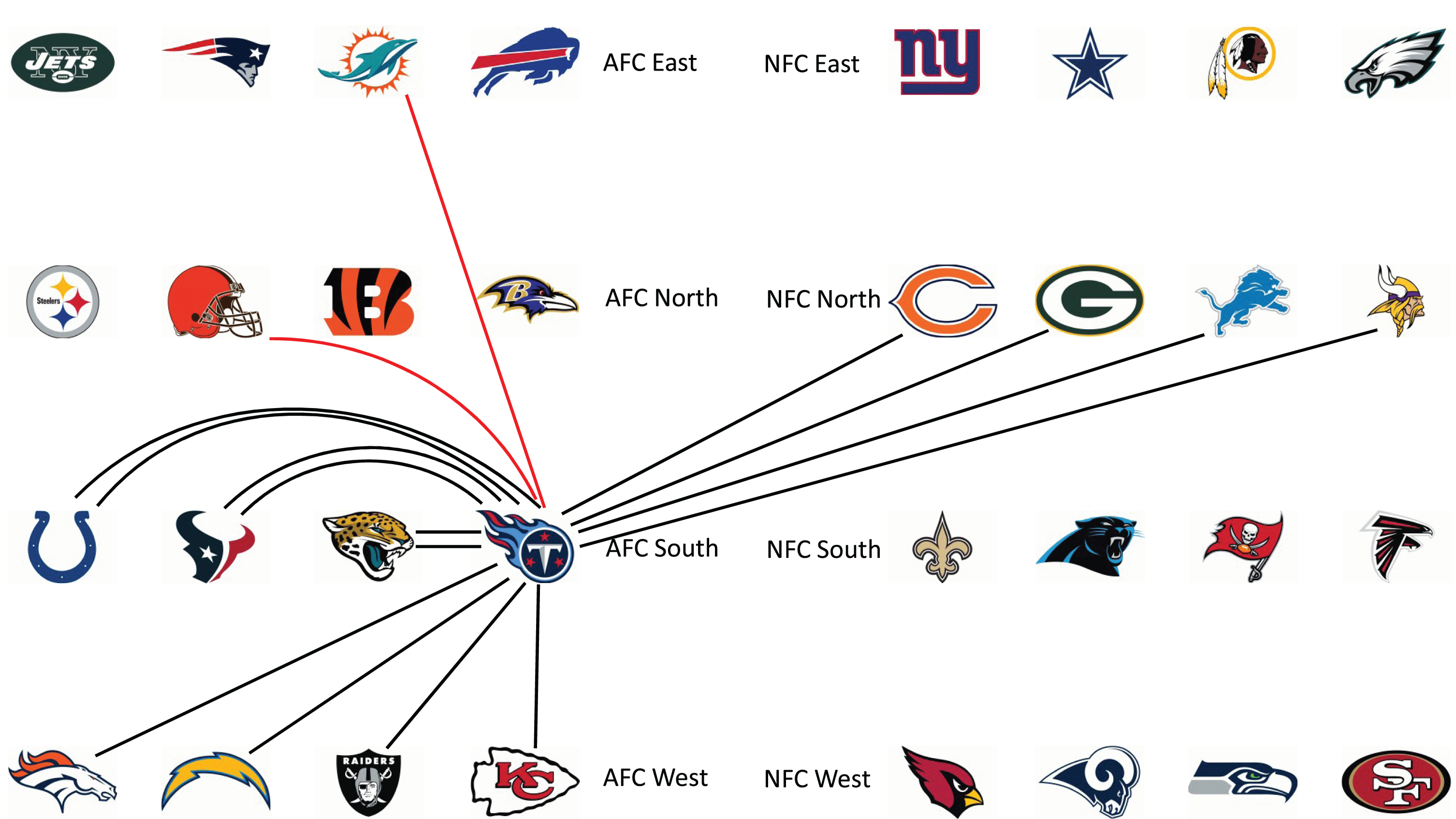
The Titans are in the AFC South, so they play each of the other teams in the AFC South twice, once home and once away. In 2016, the AFC South was matched with the AFC West and the NFC North for the remainder of their structured games. For the parity games, the Titans were matched with the Cleveland Browns in the AFC North and the Miami Dolphins in the AFC East. The Titans, Dolphins, and the Browns all finished in last place in their respective divisions in the 2015 season.
Several authors have explored aspects of the NFL schedule. Dilkina and Havens used a constraint programming approach to schedule NFL games to national television broadcasts so that the assigned games were the best possible (Dilkina and Havens 2004). Karwan, et al. were the first to study the NFL scheduling practice from the standpoint of fairness (Karwan et al. 2015). They used an integer programming approach to craft a schedule that was more equitable in terms of minimizing the maximum number of games that each team plays against more-rested opponents. Here, more-rested opponents means playing teams coming off bye weeks or teams having an extra couple of days rest from playing a Thursday night game. They also tried to equally distribute games against divisional opponents for each team. A study of Murray showed a negative impact on shorter rest periods for games won and points scored giving credence to the need for fairer scheduling practices (Murray 2018). Although this work uses a different definition of fairness, it could be combined with the work of (Karwan et al. 2015).
Here, we define fairness based on each team achieving an equalized strength of schedule. Scheduling games based on previous season’s results presents some issues because the composition and quality of a team can change dramatically from season to season. The combination of a change in team composition combined with a having to play a much harder or much easier schedule based on the parity games can dramatically change a team’s fortune. Figure 2 shows the season to season change in win totals from the 2010 to 2018 seasons.
Fig. 2
Season to season change in wins for all NFL teams from 2010–2018. Differences of at least ±4 wins account for 34% of teams and are highlighted in blue.
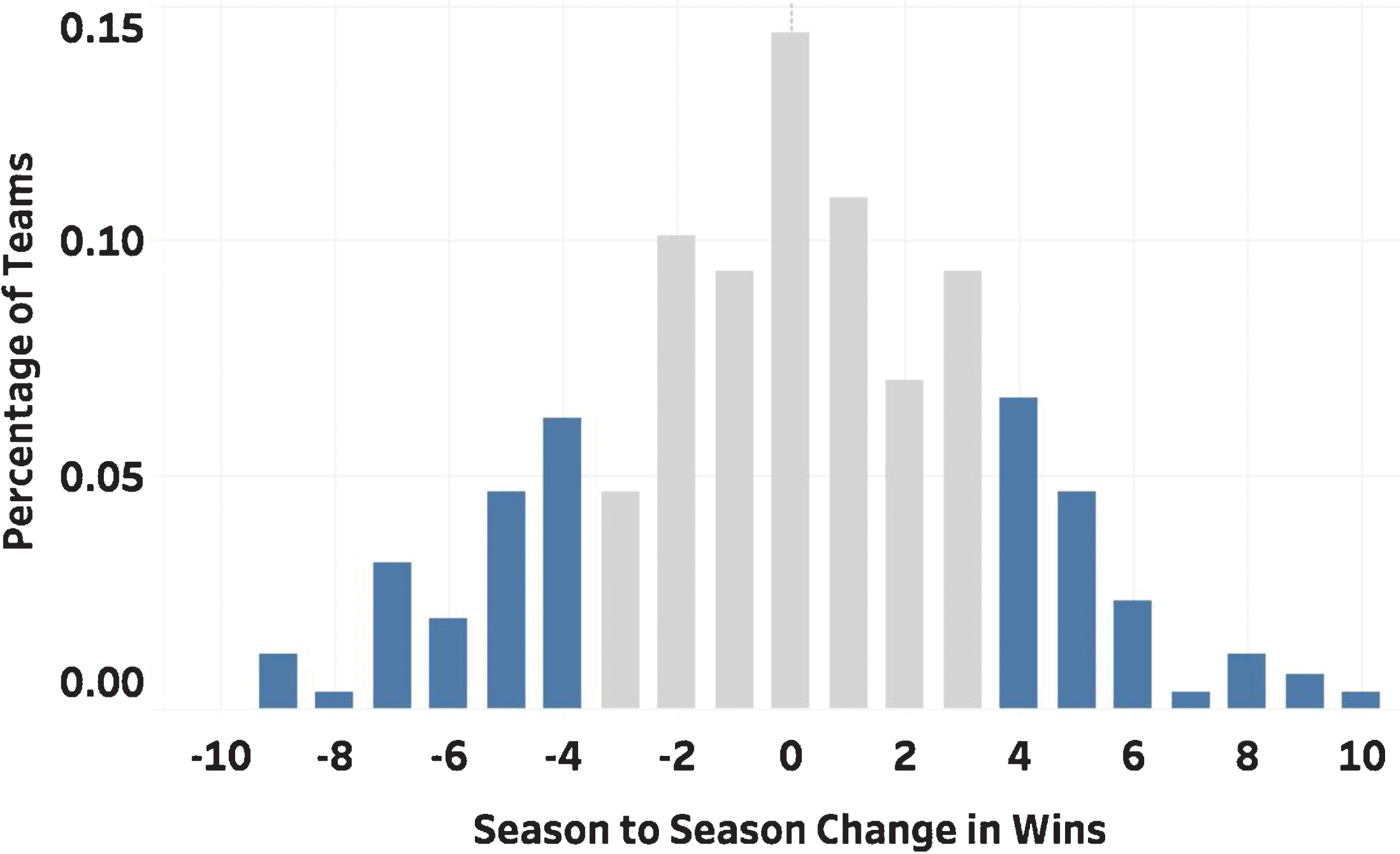
The extremes are highlighted in blue, identifying the teams that have a difference in win total of at least four games in consecutive seasons. These teams account for approximately 34% of all NFL teams during this timeframe. When considering a change of three or more wins from season to season, this increases to 48% of all teams.
At times these discrepancies in team performance have playoff implications. The 2017 Tennessee Titans tripled their win output from the previous season, begging the question as to whether the Titans were three-times better or got the benefit of an easier schedule. Table 1 shows the 2017 regular season results for five teams that were in playoff contention. Results in the table use a quality measure and a strength of schedule for each team based on their Rating Percentage Index (RPI), which is defined in Section 3. Note that Jacksonville and Tennessee made the playoffs but did so by playing a noticeably weaker schedule (strength of schedule (SOS) scores of 45.17 and 45.59 respectively) than teams with similar win-loss records (Seattle, Detroit, and Dallas), highlighting that some teams get an easier path than others to the playoffs. However, the inequities in teams’ schedule quality could be lessened by dynamically scheduling their parity games based on the current year’s results rather than basing them on the previous year’s results.
Table 1
A Comparison of 2017 Playoff Contenders
| Team | Record | Division Record | SOS | RPI | Made Playoffs? |
| Jacksonville | 10-6 | 4-2 | 45.17 | 49.51 | Yes |
| Tennessee | 9-7 | 5-1 | 45.59 | 48.25 | Yes |
| Seattle | 9-7 | 4-2 | 50.00 | 51.56 | No |
| Detroit | 9-7 | 5-1 | 51.07 | 52.36 | No |
| Dallas | 9-7 | 5-1 | 50.82 | 52.18 | No |
By removing each parity game from the data for the last six seasons (2012 through 2017), comparative statistics are computed for each team and there exists an opportunity to schedule two new games at the end of the season. The outcome of these games can be simulated to measure the improvement of dynamic schedules over those officially played. In this work, parity games are scheduled to reduce the standard deviation in the NFL’s strength of schedule in Section 4.1; reduce the number of pairwise comparisons between teams in Section 4.2; reduce the distance traveled by away teams in Section 4.3; reduce the difference in win counts between opponents in Section 4.4; and explore combinations of these objectives in Section 5.2.3.
3Basic measures of team quality
Figure 1 shows a visualization of one team’s (Tennessee Titans) schedule for an NFL season. This idea is formalized for all teams by using a graph. A graph G = (V, E) is a set of vertices (teams) V and a set of edges (games) E ⊂ V × V. In a graph, unlike Fig. 1, game (i, j) ∈ E will be a directed edge from team i to team j if team i beat team j in the season and is denoted in the visual representation of a graph by an arrow from team i to team j. Figure 3 again shows the Titans’ schedule, but as a mathematical graph reflecting win-loss information. For instance, the red arrows indicate that the Titans won both of their parity games against the Miami Dolphins and the Cleveland Browns. For the analysis in this work, graphs contain 32 vertices (one for each NFL team) and one directed edge for each game played in the season. The representation in Fig. 3 is a subgraph of the full NFL graph in that Fig. 3 only shows the Titans’ results against their opponents, not all results of all NFL games.
Fig. 3
Partial NFL graph only showing the Tennessee Titans’ opponents in the 2016 NFL season with parity games shown in red. Directed edges point from the winning team to the losing team.
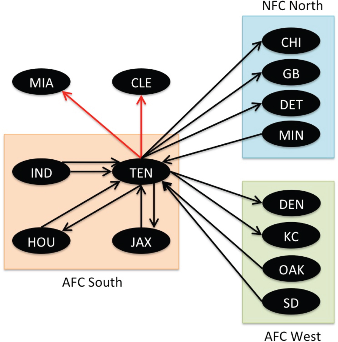
The degree d (v) of a vertex v is the number of edges incident to v. The degree can be broken down into the outdegree o (v) and indegree i (v) of v representing, respectively, the number of games won and games lost by the team. For example, in Fig. 3, d (vTEN) =16, o (vTEN) =9, and i (vTEN) =7, indicating that the Titans had nine wins and seven losses in the 2016 NFL season. A directed path P = [v0, e1, v1, e1, v2, …, ek, vk] in G is a sequence of vertices {v0, v1, …, vk} and directed edges {e1 = (v0, v1) , e2 = (v1, v2) , …, ek = (vk-1, vk)}. A directed path in a game graph allows for a chain of comparisons between teams v0 and vk since v0 beat v1 which beat v2 and so on. In Fig. 2, since Indianapolis beat Tennessee (twice) and Tennessee beat Cleveland, this path provides information to infer that Indianapolis is a stronger team than both Tennessee and Cleveland. In general, shorter paths allow for stronger comparisons of teams’ quality and longer comparison paths allow for weaker comparisons. A quality measure, or rating, can be associated with each vertex (team). For example, the winning percentage of team v is the ratio
(1)
4Game utility
This work aims to remove the parity games and add new games to the NFL schedule to improve certain metrics associated with that schedule. In effect, this would have NFL teams play a traditional schedule for the first 14 games and then play a two-game home-and-away schedule that wouldn’t be set until after the first 14 games are played. In this section several scheduling metrics are investigated that could be employed to produce desired schedules.
In testing the effectiveness of such a change, actual games played are removed and hypothetical games whose outcomes are not known are added. In adding a game between team i and team j, define the probability that team i beats team j by
(2)
Several different utilities are defined for scheduling a game between team i and team j where team i wins. Because the outcome of a newly scheduled game is unknown, the predictive utility,
(3)
4.1Strength of schedule utility (SD)
Within the RPI calculation there are two strength of schedule measures. The first, OWPi is weighted twice as much as the second, OOWPi. Keeping this convention, define a team’s strength of schedule (SOS) as
(4)
Given a set of games, generate a set S = {si|1 ≤ i ≤ 32} of strength of schedule scores. The proximity of teams’ strength of schedules can be identified by computing the standard deviation of the set S, σS. To add games to the schedule, measure the SOS utility of a game between team i and team j by measuring how the set of SOS scores changes after a new game is played, creating set Sij of 32 strength of schedule scores after a game between teams i and j is added. Lastly, define the utility of scheduling a game wherein team i beats team j as the difference of the standard deviations:
(5)
One goal in dynamically scheduling these last two games is to reduce the standard deviation after adding games, so games with large uij values are desirable. Methods for finding the 16 games with the maximum total predictive utility in each of the final two weeks of the NFL season are explored in sections 5.1 and 5.2.
4.2Comparison path utility (CP)
A second utility measure associated with adding a game to a partial season would be to reduce the maximum length of a comparison path within the game graph. Each new game added reduces the shortest path between the two teams playing but might also reduce comparison paths between other teams as well. The comparison path between teams i and j is the shortest directed path in the graph G from i to j or j to i. That is, the length cij of the comparison path between teams i and j is defined as
(6)
(7)
4.3Travel distance reduction (TD)
Traveling comes with many costs with the brunt of the expenses coming from airfare and lodging. It also adversely affects performance in sports (Entine and Small 2008; Watanabe, Wicker, and Yan 2012; Samuels 2012; Leatherwood and Dragoo 2012). Being the furthest from the majority of teams, west coast teams such as the Seattle Seahawks and Los Angeles Chargers are most affected by this cost. If two possible schedules result in a minimal difference of objective values, it would be preferable to prioritize the schedule that reduces total travel.
The utility of a game under this objective is straightforward. Let dij be the distance from the stadium of team i to that of team j so that dij = dji. The travel utility of a game between teams i and j is defined as
(8)
4.4Win differential reduction (WD)
Another indication of the quality of a team is its number of wins (o (v)). Often, as with the Conference USA example in Section 1, it is attractive to the league to bolster teams’ arguments for the playoffs by having more head-to-head matchups between top teams at the end of the season. From a fan’s perspective, this is exciting and illustrates the uncertainty of outcome hypothesis (Rottenberg 1956; Neale 1964). This type of strategy is known as a power pairing strategy and has been used in debate tournaments (Silver 2017). To accomplish a power pairing strategy schedule the remaining games between teams with similar number of wins. Let wi be the number of wins that team i accrues before the scheduling of new games. The utility or win differential of a game between teams i and j is defined as
5Solution approaches
This section introduces two methods to dynamically schedule NFL games. First, a greedy heuristic is presented to quickly identify good games to schedule. Next an optimization-based approach is introduced to maximize the utility of scheduled games.
5.1Greedy approach
The first step to a greedy approach is to sort the list of every possible new game from highest to lowest SOS predictive utilities using Equation (3). Then fill out a schedule in each of the remaining two weeks of games by selecting a game provided both of the teams involved were not previously scheduled in that week. Repeat this process for the next week, disregarding games that were scheduled in the previous week. Sometimes, depending on the order of the list, this algorithm will not be able to find a complete schedule in the second week because it will try to match two teams that were already matched in the previous week. To solve this problem, execute a swap under the following guidelines. If team i and team j still need to be scheduled, find a scheduled game in the last week between teams k and l so that a game pairing between these four teams provides the largest possible utility. The results of the greedy approach are reported in Table 4 within Section 6 and offer a considerable improvement over the NFL’s official schedule in terms of equalizing teams’ strengths of schedules. An optimization approach is presented next.
5.2Mathematical programming approach
In this section a binary linear programming model is presented to dynamically schedule two games at the end of the NFL season for each team. The binary decision variable xijk is defined to be 1 if team i is home against team j during week k and 0 otherwise. As presented earlier, the predictive utilitiy
The objective function maximizes the expected reduction in league-wide team strengths of schedule. The first constraint enforces each team plays one game per week. The second and third constraints assign one home and one away game for each team during the two week dynamic schedule. The fourth constraint confirms that a matchup between two teams occurs no more than once during the dynamic schedule. The fifth constraint eliminates intra-divisional games (including self games) and the last constraint identifies binary decision variables. The results of the mathematical programming approach are also reported in Table 4 within Section 6 and compared favorably to the NFL official schedule.
5.2.1Other objectives
The binary linear programming model introduced above can also be used to dynamically schedule games with additional objectives, such as a reduction in the comparison path across all teams. The comparison path utility described in Section 4.2 is calculated one game at a time rather than in batches of 16 or 32 games, and thus the utility of one edge often overrides part of the utility of another edge. The dependence of one score on the inclusion of another makes it difficult to guarantee any kind of optimal solution by this metric. Even so, it is effecient to formulate a mathematical programming model with the following comparison path objective function to accompany the constraints developed in Section 5.2:
5.2.2Additional constraints
Another solution technique variant is to convert an optimization objective function into a constraint. For example, the win differential objective introduced previously can be translated into a constraint on the maximum win differential m between teams scheduled to play and added to the optimization framework. Table 4 within Section 6 contains the results when dynamically scheduling to maximize the reduction in the standard deviation of league wide strengths of schedule while the win differential among teams is constrained to be no more than m = 3 and m = 4 for the 2015–2017 NFL seasons.
5.2.3Multi-objective optimization
In previous sections the motivation is presented for maximizing the reduction of the standard deviation of strengths of schedules and the comparison paths among teams, as well as the minimization of travel distances and win balancing deviations. It is of interest to consider the optimization of a multi-objective function to simultaneously consider each objective. Each of the utilities, e.g.,
6Testing and results
This section presents the simulation to evaluate the scheduling methods of the previous section. Additionally, the comparative results between dynamically scheduled games and the official NFL schedule are discussed. While the winner for each game played in previous official NFL schedules is known, the final outcomes of our scheduled games are indeterminate. Therefore, a simulation of the scheduled game and identification of the winner is based on the probability defined by Equation (2) in Section 4.1. For each of the 16 new games, generate a random number n ∈ [0, 1] and if n < pij, team i wins the game; otherwise, team j is the winner. Ties are not considered. Because margin of victory and other complicated statistics are not represented in any of the necessary calculations, this simple simulation is sufficient for this study. The simulation is repeated for 10,000 iterations and the results are averaged and compared to the official schedule below.
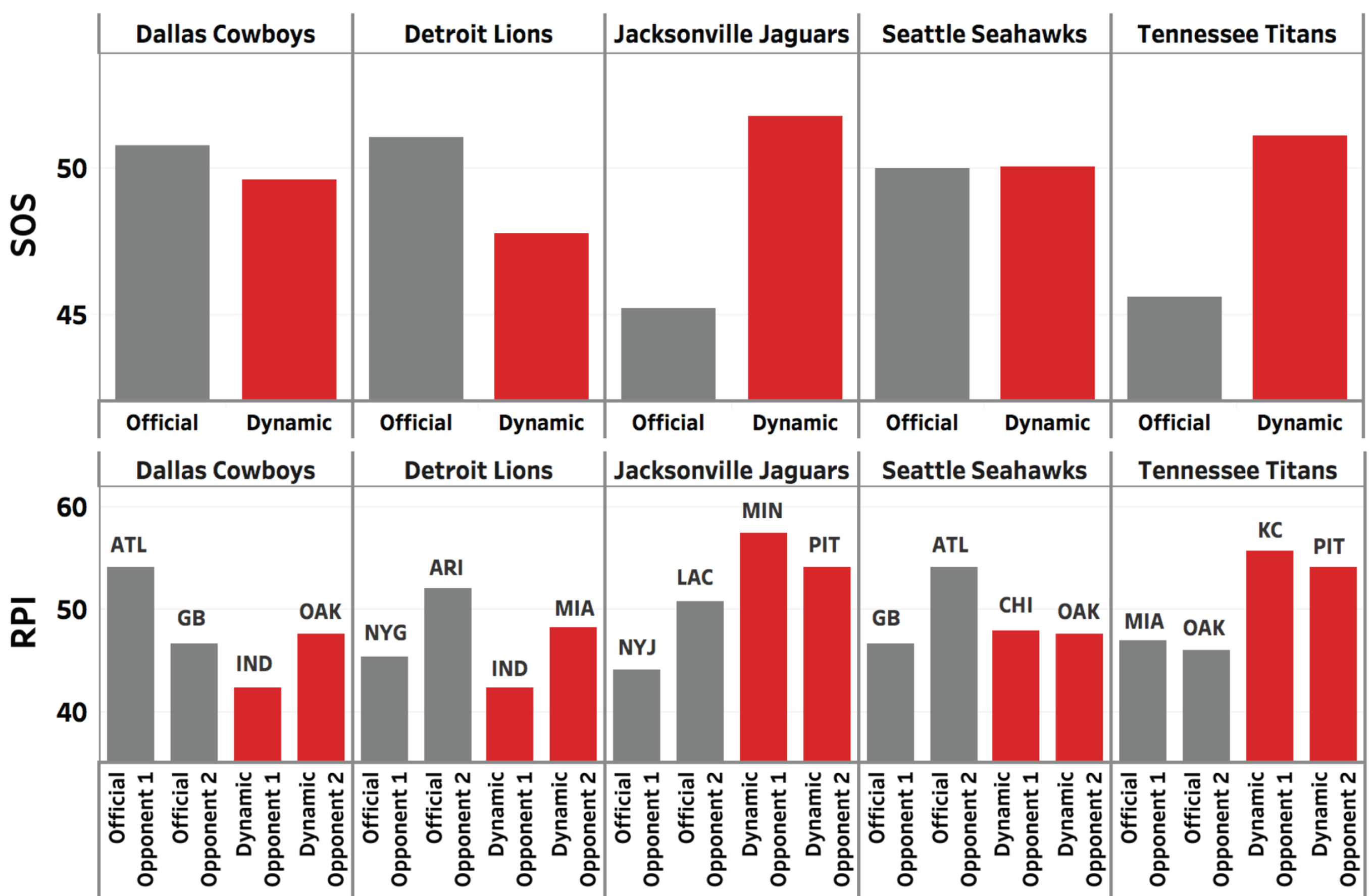
Figure 4 shows the comparison of strength of schedule for teams playing the official 2017 NFL schedule (gray) versus playing the optimized schedule (red) found via mathematical programming. As seen, the dynamically-scheduled season exhibits a reduction in the variation in strength of schedules for the league. The reduction requires some teams to play a harder schedule while others are offered an easier schedule. Figure 5 highlights the trade-off in schedule difficulty amongst Jacksonville and Tennessee (harder) and Detroit and Dallas (easier). Seattle, which was closer to a median strength of schedule of 50 initially experiences only a slight change to its schedule difficulty.
Fig. 4
Comparison of the official (gray) and dynamic (red) schedules for the 2017 NFL season.
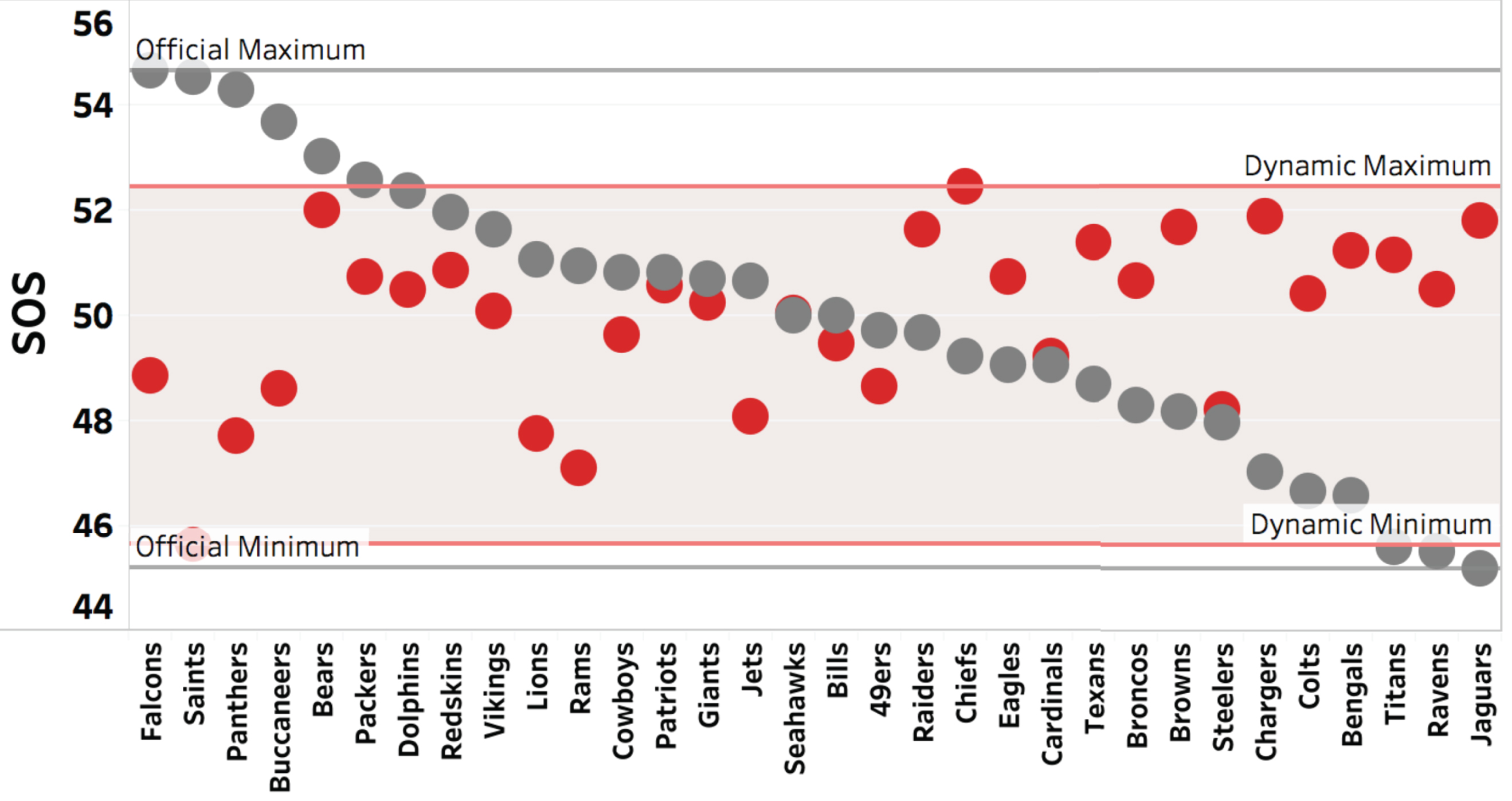
Fig. 5
Simulated change in SOS for selected teams in 2017.
Next, Table 2 shows average strength of schedule of each of the eight divisions of the NFL without the parity games, as well as the average RPI of the teams that were scheduled in the parity games to better balance the strengths of schedules. The NFC East, NFC South, and NFC West divisions had the toughest schedules that season on average. The toughest divisions received the weakest opponents based on average RPI statistics in the new schedule. In a similar manner, the divisions with the easiest schedules (the AFC North and AFC South) get much harder opponents on average in the parity games. The results presented above in Table 2, Fig. 4, and Fig. 5 present the balancing and trade-offs when scheduling NFL parity games to reduce variation in strength of schedule.
Table 2
Parity games by division
| Division | Avg SOS | Parity Games Avg RPI |
| AFC East | 50.34 | 50.69 |
| AFC North | 45.77 | 55.80 |
| AFC South | 47.80 | 54.78 |
| AFC West | 49.20 | 54.16 |
| NFC East | 52.14 | 46.69 |
| NFC North | 49.82 | 50.41 |
| NFC South | 52.62 | 43.54 |
| NFC West | 52.29 | 43.91 |
Another interesting scenario in the 2017 season involves the Philadelphia Eagles, who won the Super Bowl after finishing last in the NFC East in the previous 2016 season. The Dallas Cowboys, with a 9-7 record, challenged the Eagles, with a record of 13-3, for the division title, but because the Cowboys had finished in first place in the NFC East in the previous season, the Cowboys played a tougher schedule than the Eagles. In the parity games the Eagles played the Chicago Bears (RPI 45.47, six fewer wins) and Carolina Panthers (RPI 54.46, one fewer win) while the Cowboys played Green Bay (RPI 50.35, two fewer wins) and Atlanta (RPI 54.04, one more win). Dallas lost both of its parity games while the Eagles won both of its parity games, accounting for the four game difference in team records. Table 3 shows the games that each of dynamic scheduling methods would have scheduled for the Eagles and the Cowboys. In contrast to the strength of schedule method, because the NFC East was strong in 2017 both Philadelphia and Dallas receive lower RPI opponents, the methods that assign opponents based on win differential or some balance of win difference and strength of schedule give the Eagles and the Cowboys more competitive games. Table 3 shows the results of binary linear programming to minimize the win differential amongst all parity games (IPWDmin) and a multi-objective approach that weighs strength of schedule and win differential equally (MultiObj). In two of the three methods, the Eagles play a tougher parity-game schedule than the Cowboys as indicated by the average RPI of the opponents, and the potential outcomes of such games could have made a difference in the selection and seeding of the playoffs.
Table 3
Eagles and Cowboys parity games
| Philadelphia | Dallas | |||||
| Opponent | RPI | Win Diff | Opponent | RPI | Win Diff | |
| Chicago | 45.47 | –6 | Green Bay | 50.35 | –2 | |
| Official | Carolina | 54.46 | –1 | Atlanta | 54.04 | +1 |
| Average | 50.07 | –3.5 | Average | 52.20 | –0.5 | |
| Baltimore | 46.64 | -4 | Indianapolis | 42.3 | –5 | |
| SOS | Cincinnati | 45.27 | –6 | Oakland | 47.59 | –3 |
| Average | 45.96 | –5 | Average | 44.95 | –4 | |
| Minnesota | 57.88 | 0 | Kansas City | 53.33 | +1 | |
| IPWDmin | New England | 58.08 | 0 | New Orleans | 59.28 | +2 |
| Average | 57.98 | 0 | Average | 56.31 | +1.5 | |
| Kansas City | 53.33 | –3 | Carolina | 54.46 | +2 | |
| MultiObj | New England | 58.08 | 0 | New Orleans | 59.28 | +2 |
| Average | 55.71 | –1.5 | Average | 56.78 | +2 | |
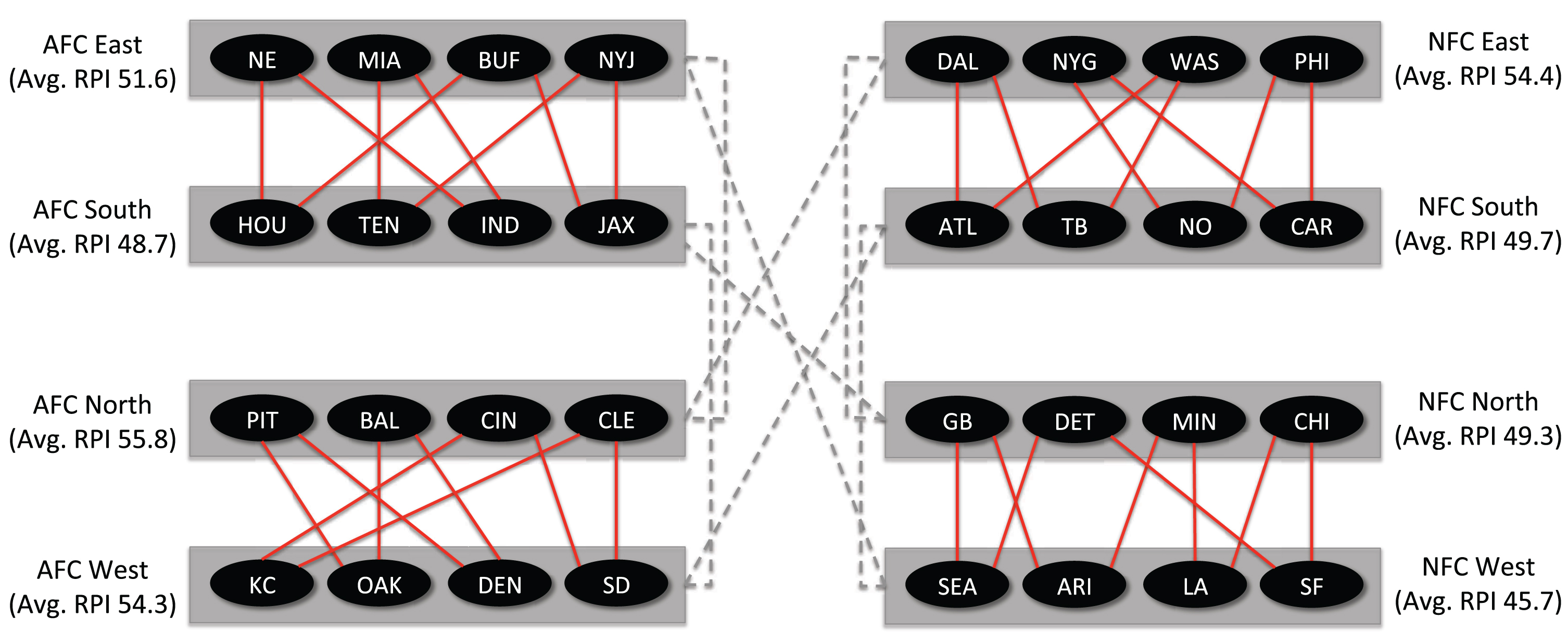
A similar phenomenon happened in the 2016 season where Detroit (9-7) made the playoffs over two other teams, Washington (8-7-1) and Tampa Bay (9-7). Detroit won its two parity games against the Los Angeles Rams (4-12) and New Orleans (7-9). Washington lost both of its parity games against Carolina (6-10) and Arizona (7-8-1). Tampa Bay split its games, winning against Chicago (3-13) but losing to Dallas (13-3). Under the dynamic schedule to equalize strength of schedule amongst teams, Detroit plays Washington (8-7-1) and Houston (9-7); Washington plays Detroit (9-7) and Minnesota (8-8); Tampa Bay plays Jacksonville (3-13) and the Los Angeles Rams (4-12). Tampa’s easier schedule makes it more likely for them to reach a 10-6 record and make the playoffs. Under a simultaneous consideration of strength of schedule and win differential through multi-objective optimization, Detroit plays Indianapolis (8-8) and Washington (8-7-1); Washington plays Detroit (9-7) and Pittsburgh (11-5); Tampa Bay plays Houston (9-7) and Tennessee (9-7). Both optimization-based methods dynamically schedule a Washington versus Detroit matchup, thereby making that game a pre-playoff playoff game to see who is worthy for the post-season. For four of the five years tested, the comparison path method of dynamic scheduling assigning teams in one division to play teams in another division in which those teams did not play during the non-parity games schedule. For example, Fig. 6 shows the parity games assigned by the comparison path method for the 2016 NFL season. The gray dotted lines represent the division matchups that were scheduled that year by the official NFL schedule and the red lines represent the parity games assigned by the optimization technique. For this year, each division was at most two steps away from another division in the network after the non-parity game schedule is played. Since the comparison path method is trying to gain comparison information by reducing the path lengths needed to compare any two teams, it seems reasonable that assigning parity games to matchup teams in one division with a division it did not play during the non-parity game schedule would accomplish this goal. Interestingly, this method seems to be assigning these intra-divisional games to pair divisions who did not play each other with similar divisional RPI scores. Using the official NFL scheduling approach, the network created from the non-parity games will naturally have short comparison paths, so this method may not be able to drastically improve on the information gained from adding these parity games. However, it is believed that the comparison path method will have great benefit in determining the quality of teams when applied to a sparser network, such as the network created from a typical college football season.
Fig. 6
Games assigned by the comparison path method and official schedule for the 2016 NFL season.
Lastly, Table 4 shows the percent improvement of each model over the statistics of the official schedule averaged over the six years studied. Note that the win balancing (WB) models are only averaged over the three years from 2015 to 2017 for m = 3 and 4. Consider the second column of the table labeled “SOS". The greedy heuristic reduces the standard deviation of the strengths of schedule by 38.6% and the mathematical programming approach further tightens the deviation to a 41.2% reduction. In a similar manner, the comparison path reduced model has the largest (2.2%) impact on the percent improvement of the comparison path of the official schedule, albeit not significant. The travel distance and win differential models also result in 11.4% and 9.5% improvements over the travel distance and win balancing metrics of the official NFL schedule, respectively. The reduction in quality of solution can be seen by balancing win differential in the row labeled “WB* m = 4". Finally, the multi-objective model results are presented with weights recorded for each of the four objectives under consideration. The multi-objective model that weighs a reduction in standard deviation of strength of schedule three times as important as minimizing travel distance, and weighs comparison path and win differential reduction twice as important as travel distance (MO (3,2,1,2)) shows improvement across all metrics compared to the official NFL schedule. In summary, the results in Table 4 come from rescheduling only two games per team. By dynamically rescheduling more games, it is reasonable to expect improvement to increase.
Table 4
Percent improvements of dynamic scheduling over the official NFL schedule
| Percent Improvement | ||||
| Model | SOS | CP | TD | WD |
| SOS Greedy | 38.6% | –11.3% | 2.1% | 0.7% |
| SOS IP | 41.2% | –10.8% | 3.0% | 0.8% |
| CP Reduced | 5.0% | 2.2% | 0.6% | 3.0% |
| TD Minimized | 6.4% | –6.5% | 11.4% | 0.1% |
| WD Minimized | –2.5% | –2.3% | 0.7% | 9.5% |
| WB* m = 4 | 28.8% | –9.2% | 2.8% | 3.5% |
| WB* m = 3 | 19.4% | –11.6% | 2.2% | 5.1% |
| MO (3,2,1,2) | 20.4% | 1.2% | 4.5% | 4.5% |
| MO (2,2,1,3) | 7.6% | 1.3% | 3.8% | 6.1% |
| MO (2,3,1,2) | 8.3% | 2.3% | 2.2% | 5.5% |
| MO (1,0,0,1) | 24.4% | –10.4% | 1.0% | 6.4% |
7Conclusion
Creating a fair schedule is important to all stakeholders of a sports league, mostly due to the financial implications of postseason participation and success. Schedule-making is a complex process requiring numerous variables and objectives to be articulated and balanced each season. The approach to scheduling traditionally used by the NFL is a static heuristic that is executed before the season and is dependent on stale information. However, as highlighted in this work, scheduling before the season based on the previous year’s results does not take into account the change in team performance due to roster and coaching changes, injuries, or many others factors. Since the schedule dictates the matchups of the season and therefore affects the composition of the postseason, it is an important problem to study how to dynamically schedule games based on the current season to more confidently identify the best teams and league champion.
This paper introduces an approach to dynamically schedule a season of NFL games to improve the fairness of the league schedule. To calculate the fairness of a schedule the quality measures among opposing teams such as Rating Percentage Index and winning percentage must be compared. Since there are many possible combinations of games to consider adding to the schedule, the utility of a potential game is used to identify better, or more fair, matchups. Several different objectives can be derived to build schedules in a systematic way to promote fairness. For example, this work examines methods to reduce the variability of teams’ strength of schedules and reduce the length of the comparison path among teams. Additionally, schedules that reduce travel distance and better balance win totals amongst opponents are presented. A simple greedy heuristic as well as mathematical programming are used to efficiently identify the best parity games to schedule each season. As shown here, scheduling based on these objectives, and combinations thereof, promote more fair and competitive schedules comparatively to recent official NFL schedules. There are further issues that need to be considered in expanding this work. First, weighting games week-to-week would reflect the trajectory of teams during the season and account for personnel changes and key injuries. Stadium availability is another concern for scheduling the unknown parity games. The feasibility of reserving a multi-purpose venue for two consecutive weeks but using only one at the end of the season could present problems, and teams, such as the New York Giants and the New York Jets who share time at the same stadium, would require additional constraints to model. Further, broadcast television contracts contribute heavily to the revenue of the NFL. Currently, considerations are made when creating the official schedule to ensure that marquee matchups occur each week. While the Win Differential objective would frequently ensure quality matchups, the other objectives would not always achieve this criteria. Preferences provided by the different television broadcasters or quality measures for potential matchups could be added to the model either in the objective function or constraints to take these preferences into consideration. Lastly, the results are tied to the optimization framework introduced in Section 5.2. It is important to acknowledge that additional constraints would most likely be needed to use dynamic scheduling in a real setting. For example, two additional realistic constraints on dynamically scheduled games are 1) opponents need to be in the same conference due to current playoff rules pointing to winning percentage amongst conference teams as a tie breaker for wild card selection and 2) teams need to have not played against one another in the previous 14 games of the schedule. However, the results of this study are promising and encourage future work to examine the effects of dynamically scheduling a portion of a league’s season.
References
1 | Dilkina B.N. , & Havens W.S. , (2004) , The U.S. National Football League Scheduling Problem, In: Association for the Advancement of Artificial Intelligence, 814-819. |
2 | Entine O.A. & Dylan S.S. , (2008) , The Role of Rest in the NBA Home-Court Advan-tage, In: Journal of Quantitative Analysis in Sport 4.2. |
3 | fivethirtyeight.com 2017, 2017 NFL Predictions. Accessed: 2020-04-02. |
4 | Karwan M , et al., (2015) , Alleviating Competitive Imbalance in NFL Schedules: An Integer Programming Approach, In: 9th Annual MIT Sloan Sports Analytics Conference. |
5 | Landon C , (2018) , C-USA making big moves in hoops, Accessed: 2019-07-12. |
6 | Langville A.N. & Meyer C.D , (2012) , Who’s #1?: The Science of Rating and Ranking, Princeton University Press. |
7 | Leatherwood W. & Dragoo J. , (2012) , Effect of Airline Travel on Performance: A Review of the Literature, In: British Journal of Sports Medicine 47.9. |
8 | Murray T , (2018) , Examining the Relationship Between Scheduling and the Outcomes of Regular Season Games in the National Football League, In: Journal of Sports Economics 19: (5), 696–724. |
9 | ncaa.com 2018, The NET, explained: NCAA adopts new college basketball ranking to replace RPI. Accessed: 2018-11-30. |
10 | Neale W.C , (Feb. (1964) ). The Peculiar Economics of Professional Sports*. In: The Quarterly Journal of Economics 78: (1), 1–14. issn: 0033-5533. doi: 10.2307/1880543. eprint: https://academic.oup.com/qje/article-pdf/78/1/1/5246371/78-1-1.pdf. url: https: //doi.org/10.2307/1880543. |
11 | nfln.com 2018, Creating the NFL Schedule. Accessed: 2018-07-12. |
12 | Rottenberg S , (1956) , The Baseball Players’ Labor Market, In: Journal of Political Economy 64: (3), 242–258. doi: 10.1086/257790. eprint: https://doi.org/10.1086/257790. URL: https://doi.org/10.1086/257790. |
13 | rpiratings.com 2018, What is RPI. Accessed: 2018-07-12. |
14 | Samuels C.H. , (2012) , Jet Lag and Travel Fatigue: A Comprehensive Management Plan for Sport Medicine Physicians and High Performance Support Teams, In Clinical Journal of Sport Medicine 22: (3), 268–273. |
15 | Silver N , (2017) , Make College Football Great Again, Accessed: 2019-07-12. |
16 | Watanabe N. , Wicker P. & Yan G. , (2012) , Weather Conditions, Travel Distance, Rest, Running Performance: The 2014 FIFA World Cup and Implication for the Future. In: Journal of Sport Management 31: (1), 27–43. |


