
Winning tennis matches with fewer points or games than the opponent
Abstract
Due to its unique scoring system, in tennis it is possible to win a match with fewer points or fewer games than the opponent. This scoring quirk has been called Quasi-Simpson paradox (QSP) and has been analyzed by Wright et al. (2013) for the years 1990–2011. This work follows up that of Wright et al. (2013) and extends it in that: i) the QSP is studied for different, and more recent, years (2012–2017), allowing a time comparison; ii) QSP is considered with respect to games as well as to points; iii) it considers both men and women; iv) the significance of the results is verified by means of statistical tests; v) it analyzes also the difference of won points, between the winner and the loser, when QSP occurs; vi) QSP is studied also through Monte Carlo simulations allowing to analyze QSP excluding any possible players’ strategy. The simulative approach allows us to solve the seeming “Federer paradox”.
1.Introduction
A tennis match comprises two to five sets. A set consists of games, and games, in turn, consist of points. The match is won by the player who first wins 2 sets in a "best of three" match or 3 sets in a "best of five" match. To win a set a player must win at least 6 games, with at least 2 games more than the opponent. In tournaments where the tie-break applies, at the score of 6-6 a seven-point game concludes the set. Finally, to win a game a player must win at least 4 points, with at least 2 points more than the opponent.
This triple nested scoring system implies that not all points weigh in the same way. As a consequence, occasionally, the loser can win more points, or also more games, than the winner. This scoring quirk has been called “Quasi-Simpson paradox” (QSP henceforth).
Tennis is not the only sport in which QSP can occur: all sports having a “best of N” scoring system, as for example volleyball and table tennis, are subject to QSP. {Moreover, some specifications of QSP are present also in other sports; see, for examples, Wardrop (1995) or Matheson (2007). However, the three-level scoring system of tennis allows QSP to appear at different stages.
The first and – to the best of our knowledge – also the unique work that considered this scoring quirk was that of Wright etal. (2013). In their paper they analyzed 61, 000 professional tennis matches of men players, from 1991 to 2011. They found that, globally, 4.52% of matches were identified as instances of QSP. They also analyzed the number of winning and losing QSP instances for 72 players, with at least 20 QSP matches in their career. Surprisingly, they found that the tennis legend and multiple record holder, Roger Federer, is the leading example of a winning loser in the sense that he lost most of the QSP matches played in his career. This was defined the Federer paradox and led some websites to claim sentences like “What Every Pro Tennis Player Does Better Than Roger Federer”1
Wright etal. (2013) and several specialized magazines and websites (for example Lawrence 2013) suggest that the occurrence of QSP in professional tennis matches can be due to a micro-level strategy of players. According to this explanation, some players choose to exert less efforts during specific periods of a match because they feel more convenient to rest and save energies. This kind of strategy should apply mainly to powerful servers who, especially after obtaining break, might prefer not to spend too much energy during the opponent’s service game. To support this explanation an interview with John Isner is often quoted, where the player explained he often adopts this strategy. However, that of the American giant can be considered a limit case, because the importance of the service in his tennis is huge and this can justify such a choice. In general, however, it is questionable whether this strategy can be applied to the majority of professional players, used to play any point as it is.
Another, simpler, explanation of this phenomenon is its statistical nature that, jointly with the tennis scoring system, implies a given percentage of occurrences of QSP. To consider this viewpoint, in this paper we analyze the QSP in tennis using both real and simulated data.
The present work follows up that of Wright etal. (2013) and extends it because: i) the QSP is studied for different, and more recent, years (2012–2017) allowing also a time comparison; ii) QSP is considered with respect to games as well as to points; iii) it considers both men and women; iv) the significance of the results is verified by means of statistical tests; v) it analyzes also the difference of won points, between the winner and the loser, when QSP occurs; vi) QSP is studied also through Monte Carlo simulations thus warranting the observation of QSP excluding any possible players’ strategy or specific features; vii) it gives an explanation of the seeming “Federer paradox”.
Differently from Wright etal. (2013), we did not consider differences among surface types, except when performing tests on their results.
The rest of the paper is organized as follows: in Section 2 the datasets used in this work are described; Section 3 contains the description of the statistical test applied to assess the significance of differences. The analyses of QSP for real matches, both for men and women, are carried out in Section 4. In particular, Sections 4.1 and 4.2 consider, respectively, the QSP at points and games level, while Section 4.3 concerns the difference of points in case of QSP. Section 5 is devoted to Monte Carlo simulations, under the hypothesis that points are i.i.d. Analyses at individual-level are carried out in Section 6. An overall discussion and conclusions are given in Section 7.
2.The datasets
This work analyzes instances of QSP in professional tennis matches, with respect to points and with respect to games, both for men and women. When analyzing the QSP in games, only the final scores are needed. This kind of information is easy to find and we retrieved it from the tennis-data website2
For men, the final scores of all the matches played in the ATP world tour from January 2000 to March 2017 have been downloaded. These include the Grand Slam championships, all played best of five sets, and the Master 1000, the ATP500 and ATP250 tournaments, played best of three sets. Davis Cup’s matches have not been included. The total number of matches for men is 46, 083, of which 8, 509 are played at best of five sets and 37, 574 at best of three sets. The best of three sets matches are further divided in two classes: the Master 1000 matches (9, 689) and the union of ATP500 and ATP250 matches (27, 885). This classification is motivated by the decreasing importance of tournaments.
Likewise, for women we considered all the data available on the website, which cover the Grand Slam championships, the Premier and the International tournaments for the period January 2007 – March 2017. The total number of matches is 26, 008, of which 5, 461 refer to Grand Slam’s matches, 9, 884 to Premier’s matches and 10, 663 to International’s matches. For women all tournaments are played best of three sets.
To analyze QSP at points level, we need to know the number of points won and lost by the two players in each match. This piece of information was not available in the tennis-data website, thus we retrieved it from the OnCourt database3 . For this analysis all the matches in the period January 2012 – March 2017, both for men and women, have been considered. For men, this amounts to 11, 353 matches, of which 4, 453 are Grand Slam’s matches, 3, 847 are Master 1000’s matches and 3, 053 are ATP500 or ATP250 matches. For women, there are 8, 868 matches, composed by 2, 622 Grand Slam’s matches, 3, 174 Premier’s matches and 3, 072 International’s matches.
We have chosen to study QSP at points level for this relatively short period because the period 1990 – 2011 was already studied by Wright etal. (2013). In Section 4.1, their results will be compared with ours to evaluate the time evolution of the phenomenon.
3.Assessing significance
A distinctive feature of this work is the use of statistical tests to assess the significance of differences between observed percentages of QSP occurrences. The probability of the occurrence of a given number of QSP in n matches can be described by a binomial distribution, Bin (n, p) where p is the “true” probability that a QSP arises.
Now, suppose we have k samples of sizes n1, . . . , nk each from an independent binomial distribution Bin (ni, pi) (i = 1, . . . , k). Let si and
(1)
The maximum likelihood estimators of pi and p are
(2)
4.Real data
4.1.Winning with fewer points
In this section, the occurrence of QSP at points level (QSP-P from now on) is analyzed. Thus, we count how often a player wins a match with fewer points than his/her opponent or, equivalently, how often a player loses a match winning more points than his/her opponent.
From now on, for the sake of simplicity, best of three and best of five sets matches will be referred to as Bof3 and Bof5.
Percentage occurrences of QSP-P for men are listed in Table 1, divided for type of tournament. Although years and matches are different from those considered by Wright etal. (2013), the percentage of total matches that exhibit QSP-P, 4.41%, is incredibly close to that found by Wright etal. (2013), which was 4.52%. Thus, although infrequent, QSP-P is not a so rare event in tennis as other ones (O’Donoghue 2013). In Grand Slam matches, coinciding with Bof5 matches, QSP-P occurs only 4.02% of times. The percentage increases to 4.42% for ATP500 or ATP250 matches and to 4.89% for Master 1000 matches. The weighted mean for Bof3 matches is 4.68%.
Table 1
Men: percentage of matches won with fewer points than the opponent
| Tournament | n. of matches | Percentage |
| Grand Slam | 4,453 | 4.02 |
| Master 1000 | 3,847 | 4.89 |
| ATP 500/250 | 3,053 | 4.42 |
| Total | 11,353 | 4.41 |
| Best of 5 | 4,453 | 4.02 |
| Best of 3 | 6,900 | 4.68 |
For our data, occurrence of QSP-P is more frequent in Bof3 than in Bof5 matches, which is the opposite of what Wright etal. (2013) found. However, when testing the significance of the differences between the two percentages, using test (2), a p-value of 0.103 is obtained. Thus, this difference is not statistically significant.
Putting together our results with those in the literature has allowed us to analyze and test the time evolution of QSP-P. The first three rows of Table 2 contain the percentage values observed by Wright etal. (2013), while the fourth row shows the percentage found in this work. The global average percentage of QSP-P, weighted by the number of matches in each period, is also shown. The percentages in the four periods range from 4.18 to 4.78, without highlighting any specific pattern. The hypothesis that there is no difference among the occurrence probabilities in the four periods has been assessed through the LR test. This has led to a p-value close to 1, so that differences among periods are highly not significant.
Table 2
Men: percentage of QSP occurrence at points level for different periods. Results for the period 1991–2011 are those of Wright etal. (2013)
| Period | n. of matches | percentage |
| 1991–1997 | 23,053 | 4.78 |
| 1998–2004 | 20,037 | 4.53 |
| 2005–2011 | 18,699 | 4.18 |
| 2012–2017 | 11,353 | 4.41 |
| Weighted average | 4.50 |
In their paper, Wright etal. (2013) analyzed QSP-P also in four types of surfaces: carpet, clay, grass and hard. They found that the percentages of instances of QSP-P for these surfaces are 4.54%, 4.31%, 4.92% and 4.57%, respectively. Despite the slightly higher percentage for grass, the test for equal probabilities leads to a p-value of 0.17. Thus, differences are not significant. We can therefore conclude that, for men players, the probability of occurrence of QSP-P does not change with surface or type of tournament and has not changed in the last 25 years. As in these years tennis equipment and materials, on the other hand, have largely changed, and the importance of service has become more and more relevant, the previous results cast a doubt on the real causes of QSP-P occurrence, suggesting that it could be nothing but a statistical scoring quirk.
Table 3 lists the empirical percentage of QSP-P instances in women matches. For women, all tournaments are played Bof3. With respect to men, results for female matches highlight two main differences: the occurrence of QSP-P is 26% lower than that for men and the difference between Grand Slam’s and other matches is more pronounced. These two features are supported also by the application of the LR test (2). Indeed, testing the equality of occurrence probabilities in Grand Slam matches and other matches, leads to a p-value of 0.033. Likewise, when comparing the overall probabilities of QSP-P in men’s and women’s matches, the resulting p-value is less than 0.001. Thus both these differences are significant at 5% significance level. As results of Section 5 show that P(QSP-P) is inversely related to the difference in the level of the players, a natural explanation could be that – on average – the difference between high-rank players and mid-or low-rank players is more important for women than for men. Typically, major tournaments involve higher-rank players, hence the difference.
Table 3
Women: percentage of matches won with fewer points than the opponent
| Tournament | n. of matches | percentage |
| Grand Slam | 2,622 | 2.63 |
| Premier | 3,174 | 3.78 |
| International | 3,072 | 3.20 |
| Total | 8,868 | 3.24 |
| Grand Slam | 2,622 | 2.63 |
| Other | 6,246 | 3.49 |
4.2.Winning with fewer games
In this section the occurrence of QSP with respect to games (from now on QSP-G) in professional players’ matches is studied. In this situation, a player wins a match winning, globally, fewer games than the opponent. To the best of our knowledge, this is the first time this specific issue has been considered.
Notice that the dataset used for QSP-G analyses is different from that used for QSP-P and it covers a much wider period of time. Absolute and percentage frequencies of QSP-G in our dataset are listed in Table 4, for men, and Table 5, for women. Table 4 also distinguishes between Bof3 and Bof5 matches.
Table 4
Men: percentage of matches won with fewer games than the opponent
| Tournament | n. of matches | percentage |
| Grand Slam | 8,509 | 1.96 |
| Master 1000 | 9,689 | 2.15 |
| ATP 250/500 | 27,885 | 2.18 |
| Total | 46,083 | 2.15 |
| Best of 5 | 8,509 | 1.96 |
| Best of 3 | 37,574 | 2.17 |
Table 5
Women: percentage of matches won with fewer games than the opponent
| Tournament | n. of matches | percentage |
| Grand Slam | 5,461 | 1.28 |
| Premier | 9,884 | 2.13 |
| International | 10,663 | 1.89 |
| Total | 26,008 | 1.85 |
| Grand Slam | 5,461 | 1.28 |
| Others | 20,547 | 2.00 |
For men, globally, QSP-G occurs in 2.15% of matches, while for women 1.85% of matches. Both for men and for women, the occurrence of QSP-G is less frequent than QSP-P. However, moving from points level to games level, the relative frequency of QSP reduces more for men (-52%) than for women (-43%). On the other hand, when considering the difference between Bof3 and Bof5 matches (for men), the reduction of the relative frequency is roughly the same (-53% and -51%, respectively).
For men, as for QSP-P, the occurrence of QSP-G in Bof5 matches is less frequent (1.96%) than in Bof3 matches (2.17%). However, test (2) yields a p-value of 0.233, suggesting that there is no difference between the probabilities of QSP-G in Bof3 and Bof5 matches.
Table 5 shows the observed percentage occurrences of QSP-G for women. QSP-G concerns 1.28% of Grand Slam matches and 2.00% of other tournaments matches. Differently from men, the LR test rejects the hypothesis of no difference with a p-value of 0.033. Thus, for matches played in the Grand Slam championships, QSP-G has a significantly lower probability to occur.
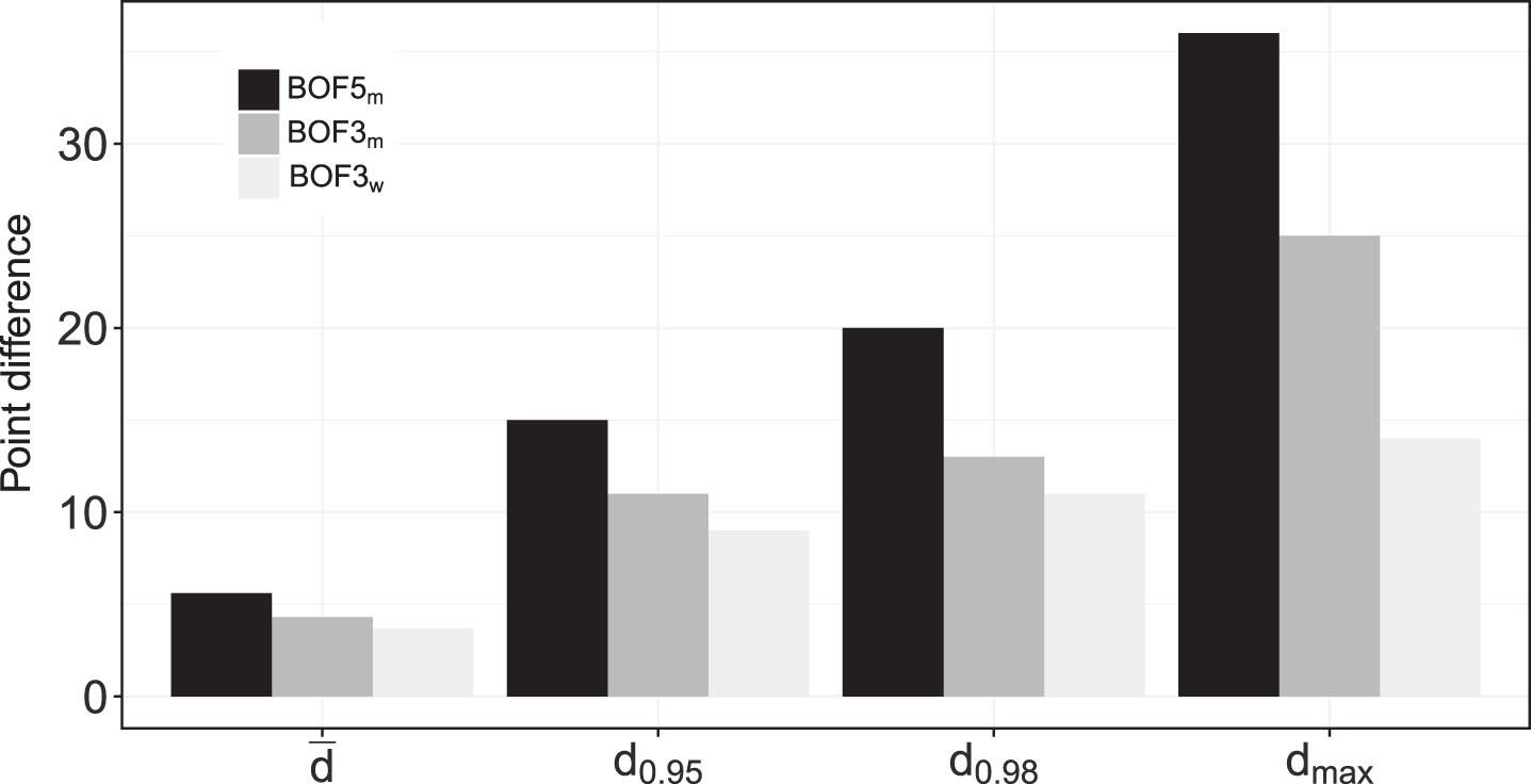
4.3.Difference of points
We further investigate QSP-P by analyzing the difference d between the number of points won by the loser and the winner when QSP-P arises. Beside d we also consider the difference in percentage of points won, dpct. For this kind of analysis, we distinguish only between Bof3 and Bof5 matches.
Table 6 lists, both for d and dpct, the mean values (
Table 6
Absolute (d) and percentage (dpctc) differences in points between winner and loser when a QSP-P occurs.
| Best of 3 sets | Best of 5 sets | |||||||
| d |
| d0.95 | d0.98 | dmax |
| d0.95 | d0.98 | dmax |
| Men | 4.3 | 11.0 | 13.0 | 25.0 | 5.6 | 15.0 | 20.0 | 36.0 |
| Women | 3.7 | 9.0 | 11.0 | 14.0 | – | – | – | – |
| dpct |
| dpct0.95 | dpct0.98 | dpctmax |
| dpct0.95 | dpct0.98 | dpctmax |
| Men | 2.3 | 5.6 | 6.8 | 11.0 | 2.2 | 5.7 | 8.0 | 19.2 |
| Women | 1.9 | 4.9 | 5.9 | 7.0 | – | – | – | – |
5.Simulations
To have a deeper insight of QSP we resort to Monte Carlo simulations (see Newton and Aslam, 2009, Baca, 2015). The use of simulations also allows us to analyze QSP excluding any possible voluntary strategy and, thus, to compare observed results with those expected under the hypothesis of absence of intentional behavior of players. Using the R environment, suitable functions that “play” probabilistic matches between players A and B have been written. The starting point is pi = Prob (Player i winsapointat service), with i = A, B. Clearly, if pA is the probability that player A wins a point at his own service, 1 - pA is the probability that player B wins a point when returning, and vice versa.
During the development of the match, we assume that points are i.i.d. conditionally on the server. Although this assumption could seem too strong, literature pointed out it can be considered a good approximation (Klaassen and Magnus, 2001).
Simulations distinguish between Bof3 and Bof5 matches, but also assume that at the 6-6 score a tie-break is always played. While it is well known this is not true for all championships4 , we do not think final results will be affected.
The probability of winning a point depends on the players’ skills to serve (servi) but also on how well their opponents return (retj), so that we can write pA = (servA - retB) and pB = (servB - retA). As these features depend on both pA and pB, one should consider different simulations for each couple (pA, pB). To summarize the results, and following Klaassen Magnus (2014), we consider two new parameters: δ = pA - pB and γ = pA + pB. Since δ = pA - pB = (servA + retA) - (servB + retB), it represents the quality difference between the two players. Likewise, as γ = pA + pB = (servA - retA) + (servB - retB), it represents the sum of serve-return difference for both players. There are two main advantages in considering γ and δ: i) they are related to each other much less than pA and pB and ii) Klaassen and Magnus showed that the probability of winning (or losing) a set or a match depends primarily on δ. In a moment we will see that in our case this is true for |δ|.
Although in principle δ can vary in (-1, 1) and γ in (0, 2), in the simulations we consider δ ∈ (0, 0.4) and γ ∈ (0.9, 1.5), which are the relevant ranges in practice. In particular, only positive values of δ are considered because in the simulations the sign of δ simply depends on which player is "player A" and, in practice, what is relevant is the absolute difference in the players’ quality.
For each given (δ, γ) couple, 20, 000 Bof3 and Bof5 matches are simulated and the percentages of QSP-P and QSP-G occurrences are recorded. By replicating the 20, 000 runs several times we found the Monte Carlo variability to be small and not affecting the conclusions.
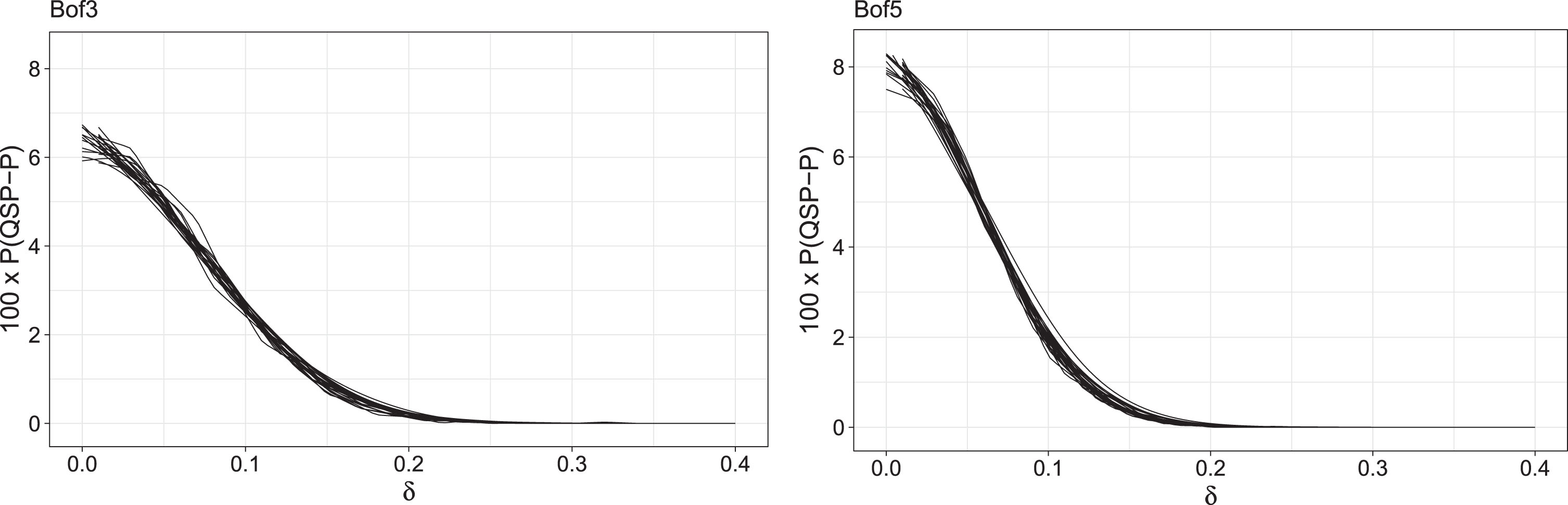
Figure 1 summarizes the results. For each given value of γ, it includes the curve describing the probability (×100) of the QSP-P occurrence as a function of δ. The collection of all curves for 0.9 ≤ γ ≤ 1.5 gives the thickness of the curve. It is clear that the probability of QSP-P occurrence depends mainly on δ and only marginally on γ, both for Bof3 and Bof5 matches. For very small δ, corresponding to almost equally strong players, the probability of the QSP-P occurrence is lower for Bof3 matches than for Bof5 matches, reaching 8%. However, in the latter case, when δ increases, this probability decreases more quickly than in the former case. As an example, for δ = 0.1 the estimated probability of QSP-P occurrence is around 2.5% for Bof3 matches and around 1.8% for Bof5 matches.
Fig. 1
Estimated probability (×100) of QSP-P based on 20,000 simulated matches. Left: best of 3; right: best of 5.
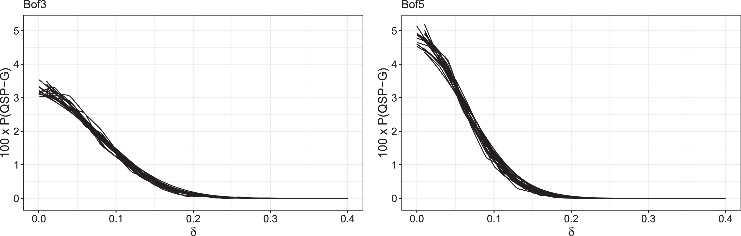
Figure 2 shows the equivalent representation for QSP-G. Also in this case the qualitative behavior of P(QSP-G) is the same as P(QSP-P) but the occurrence of QSP-G is less frequent than that of QSP-P and the difference between Bof3 and Bof5 matches is more marked.
Fig. 2
Estimated probability of Simpson’s effect with respect to games. Left: best of 3; right: best of 5.
We would also like to remark that, while the effect of γ is minor, we found that there appears to be increasing monotonicity with respect to γ, especially for the probability of QSP-P.
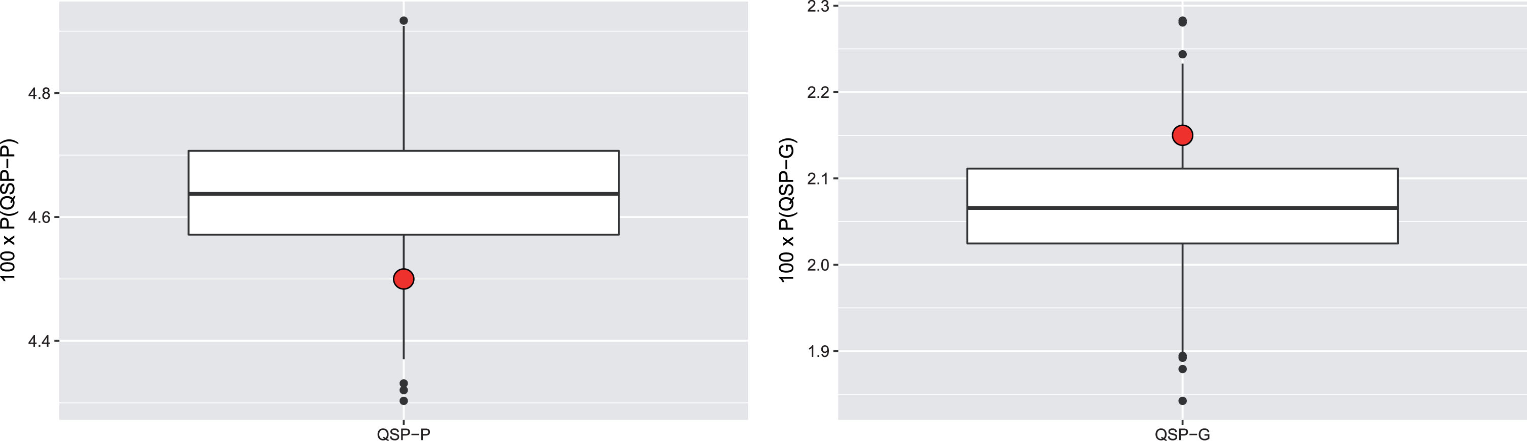
Results of simulations are useful as a benchmark for the occurrence of QSP in a framework without any strategy. Ideally, a fair comparison between empirical and simulated data would require to identify, first, average values (over all players in the ATP rankings) of pA and pB, say
Fig. 3
Distributions of P(QSP-P) (left) and P(QSP-G) (right) obtained with 1000 Monte Carlo replications of the experiment with random pA and pB. Horizontal lines correspond to 25th, 50th and 75th percentiles of the distribution. Large red dots represent the observed percentages of QSP, which lie at the 7.8th and 88.7th percentile of the P(QSP-P) and P(QSP-G) distributions, respectively.
We notice that, as Figs. 1 and 2 point out, what really matters is the value of |pA - pB| rather than the value of pA or pB themselves. Thus, considering, e.g., a U (0.55, 0.8) instead of a U (0.5, 0.75) would not change conclusions significantly. We believe that |pA - pB| ∈ (0, 0.25) is enough to describe the complex real situation, because a δ equal to 0.25 strongly affects the probability of winning the match.
The simulative approach allows to also consider another related issue: when a QSP-P occurs, how large is the point difference? In order to answer this question, 20, 000 matches are simulated and each time a QSP-P occurs the difference d in points between the winner and the loser is recorded. Even here results depend on pA and pB. In the simulations, for simplicity, we consider pA = 0.64, 0.58, 0.54 and pB = pA + 0.01, pA + 0.1, pA + 0.15, corresponding to a small, large and very large difference between the two probabilities.
The mean difference in points won by opponents when a Simpson match occurs ranges from 3.6 to 6.2, depending on pA and pB, for Bof3 matches and from 4.8 to 10 for Bof5 matches. The maximum difference in points ranges from 15 to 23 for Bof3 matches and from 23 to 34 for Bof5 matches corresponding, respectively, to around 5 games and around 6-7 games. Table 7 lists the mean value, the quantiles 0.95 and 0.98 of the distribution and the maximum observed value, for Bof3 and Bof5 matches for dpct, the difference in percentage of points won in a Simpson match. Results for the considered couples of pA and pB point out that, in percentage, there are not large differences between Bof3 an Bof5 matches and differences never exceed 12%.
Table 7
Difference in percentage of points won by winner and loser when a QSP-P occurs. Number of simulated matches: 50,000.
| Best of 3 sets | Best of 5 sets | ||||||||
| pA | pB |
| dpct0.95 | dpct0.98 | dpctmax |
| dpct0.95 | dpct0.98 | dpctmax |
| 0.64 | 0.65 | 1.9 | 4.6 | 5.6 | 10.1 | 1.5 | 3.8 | 4.6 | 7.9 |
| 0.64 | 0.74 | 2.3 | 5.6 | 6.7 | 10.7 | 2.2 | 5.5 | 6.6 | 9.6 |
| 0.64 | 0.79 | 3.0 | 7.2 | 8.3 | 11.9 | 3.1 | 6.7 | 7.5 | 10.5 |
| 0.58 | 0.59 | 1.9 | 4.8 | 5.8 | 8.7 | 1.5 | 3.8 | 4.7 | 7.5 |
| 0.58 | 0.68 | 2.1 | 5.1 | 5.9 | 9.0 | 1.9 | 4.9 | 6.0 | 8.6 |
| 0.58 | 0.73 | 2.6 | 6.4 | 7.5 | 8.8 | 2.6 | 6.2 | 6.8 | 10.0 |
| 0.54 | 0.55 | 1.8 | 4.5 | 5.3 | 9.1 | 1.5 | 3.9 | 4.7 | 8.2 |
| 0.54 | 0.65 | 2.2 | 5.4 | 6.7 | 10.2 | 2.0 | 4.7 | 5.7 | 8.0 |
| 0.54 | 0.69 | 2.5 | 6.0 | 7.1 | 9.9 | 2.5 | 5.8 | 6.4 | 8.8 |
6.Individual-level analyses
In this section we study the QSP at individual level by considering the percentage of winning (winning a match with fewer points) and losing (losing a match with more points) QSP matches, conditionally to an occurrence of QSP. The final goal is to analyze more in depth the reasons underlying the occurrences of winning and losing QSP, in particular for players with a predominance of winning (or losing) QSP. These reasons could be intentional, for example the choice of some strategy, or unconscious, for example the ability to perform well under pressure, as in this case players win the games they have to win (or vice versa). Players who often lose despite winning more points or games could be those who “choke” under pressure. However, these interpretations are not always based on clear arguments. Also, they are not so immediate because they refer to a phenomenon which, for its nature, is relatively rare and, thus, undersampled. How to explain, for example, the astonishing result found by Wright etal. (2013), that Roger Federer is the player with the worst ratio of winning/losing QSP? Does this really suggest that Federer has a poor winning attitude? And, in this case, how can this coexist with the shiny career of Federer and the incredible results he has reached over the last 15 years?
We start our analyses by updating the statistics by Wright etal. (2013). They considered 72 players that in their career played at least 20 QSP matches until the end of 2011. For each player, the total number of matches in the sample ranged from 201 to 927, with an average size of around 570 matches. We update these statistics for players who took part in at least 100 matches after 2011: we found thirteen such players, listed in Table 8. For each of these thirteen players, Table 8 lists the total number of matches in the sample, and the number and percentage of winning and losing QSP matches. These pieces of information are divided into three periods: 1991–2011 (results found by Wright etal. (2013)), 2012–2017 (new results) and the whole period 1991–2017. This allows us to study how results change in different periods and, thus, their stability as well as the effect of the sample size. In general, increasing the sample size (period 1991–2017) tends to balance the percentage of winning and losing QSP. However, there are cases for which the percentage of winning and losing QSP completely reverses in the period 2012–2017: some examples are Nadal, Isner, Stepanek and Verdasco. For Nadal the percentage of winning QSP changes from 70% over 613 matches to around 56% over 1025 matches. Likewise, for Isner, the extraordinary 80% of winning QSP over 201 matches drops to 59% over 590 matches. This suggests that the variability of these percentages is high and that only a very long sequence of matches can lead to stable results.
Table 8
Winning and losing QSP for some professional players for different periods. N.matches=total matches analyzed; WS=number of winning QSP matches; LS=number of losing QSP matches; %WS and %LS=percentages of winning and losing QSP matches with respect to the total number of QSP matches
| Years | n.matches | WS | LS | % WS | % LS | |
| Davydenko | 1991–2011 | 927 | 4 | 24 | 14.3 | 85.7 |
| 2012–2018 | 106 | 0 | 1 | 0 | 100 | |
| 1991–2018 | 1033 | 4 | 25 | 13.8 | 86.2 | |
| Federer | 1991–2011 | 927 | 4 | 24 | 14.3 | 85.7 |
| 2012–2018 | 417 | 3 | 9 | 25.0 | 75.0 | |
| 1991–2018 | 1344 | 7 | 33 | 17.5 | 82.5 | |
| Isner | 1991–2011 | 201 | 19 | 5 | 79.2 | 20.8 |
| 2012–2018 | 389 | 17 | 20 | 45.9 | 41.0 | |
| 1991–2018 | 590 | 36 | 25 | 59.0 | 44.1 | |
| Haas | 1991–2011 | 649 | 19 | 15 | 55.9 | 44.1 |
| 2012–2018 | 180 | 3 | 2 | 60.0 | 40.0 | |
| 1991–2018 | 829 | 22 | 17 | 56.4 | 43.6 | |
| Hewitt | 1991–2011 | 673 | 15 | 11 | 57.7 | 42.3 |
| 2012–2018 | 125 | 4 | 4 | 50.0 | 50.0 | |
| 1991–2018 | 798 | 19 | 15 | 55.8 | 44.2 | |
| Lopez | 1991–2011 | 499 | 21 | 6 | 77.8 | 22.2 |
| 2012–2018 | 348 | 14 | 14 | 50.0 | 50.0 | |
| 1991–2018 | 847 | 35 | 20 | 63.6 | 36.4 | |
| Monfils | 1991–2011 | 338 | 12 | 8 | 60.0 | 40.0 |
| 2012–2018 | 305 | 7 | 4 | 63.6 | 46.4 | |
| 1991–2018 | 643 | 19 | 12 | 61.3 | 38.7 | |
| Nadal | 1991–2011 | 613 | 14 | 6 | 70.0 | 30.0 |
| 2012–2018 | 412 | 4 | 8 | 33.3 | 66.7 | |
| 1991–2018 | 1025 | 18 | 14 | 56.2 | 43.8 | |
| Nieminen | 1991–2011 | 493 | 17 | 12 | 58.6 | 41.4 |
| 2012–2018 | 223 | 5 | 3 | 62.5 | 37.5 | |
| 1991–2018 | 716 | 22 | 15 | 59.5 | 40.5 | |
| Robredo | 1991–2011 | 643 | 28 | 9 | 75.7 | 24.3 |
| 2012–2018 | 285 | 8 | 5 | 61.5 | 38.5 | |
| 1991–2018 | 928 | 36 | 14 | 72.0 | 28.0 | |
| Stepanek | 1991–2011 | 488 | 11 | 9 | 55.0 | 45.0 |
| 2012–2018 | 236 | 2 | 7 | 22.2 | 77.8 | |
| 1991–2018 | 724 | 13 | 16 | 44.8 | 55.2 | |
| Verdasco | 1991–2011 | 579 | 12 | 10 | 50.5 | 45.5 |
| 2012–2018 | 337 | 5 | 14 | 26.3 | 73.7 | |
| 1991–2018 | 840 | 14 | 27 | 34.1 | 65.9 | |
| Youzhny | 1991–2011 | 503 | 9 | 13 | 40.9 | 59.1 |
| 2012–2018 | 341 | 12 | 10 | 54.5 | 45.5 | |
| 1991–2018 | 844 | 21 | 23 | 47.7 | 52.3 |
The player with the highest number of matches is Federer (1344): in this case the results for the period 1991–2017 are not so different from those of the period 1991–2011. As this latter period consisted of more than 900 matches, this is not strange. What is strange, in some sense, is that the negative record of Federer persists also in the period 2012–2017.
To better understand this negative record, we used Monte Carlo simulations to study the occurrences of winning and losing QSP. As before, this approach relies only on the probabilities of winning a point at his own service (pA and pB), while keeping out any strategy and all specific features of the two players (attitude, psychological aspects, etc.).
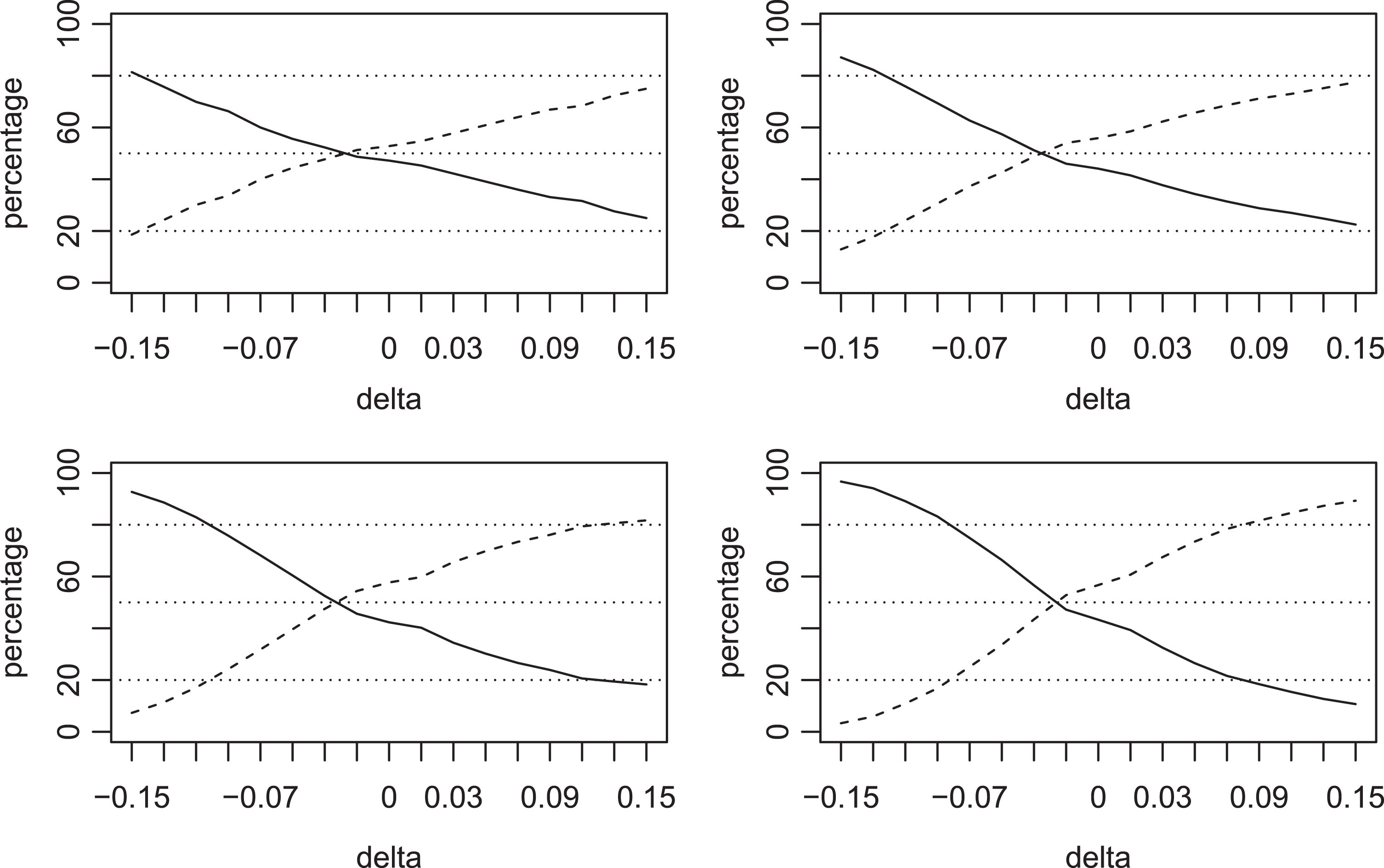
For pA ∈ 0.55, 0.60, 0.65, 0.70, and letting δ = pA - pB vary in the interval [-0.15, 0.15], we played 50, 000 matches and computed the number and the percentage of winning and losing QSP matches. Repeating the experiment several times, we found 50, 000 runs to be sufficient to make the Monte Carlo variability negligible with respect to our conclusions. The percentages are described in Fig. 4, for Bof3 matches, and in Fig. 5, for Bof5 matches. Results are very interesting; indeed, one could believe that if player A is much stronger than player B, he will experience many more winning than losing QSP (conditionally to the occurrence of QSPs). Actually, the opposite occurs. Consider, for example, Fig. 4: the four panels show the percentage of winning QSP (full line) and the percentage of losing QSP (dashed line) for pA = 0.55, 0.60, 0.65 and 0.70 - clockwise - as function of δ. Positive values of δ mean that player A is stronger than player B. As we can see, the larger δ is, the smaller the probability to observe a winning QSP match. For example, for pA = 0.65 and δ = 0.15 the expected percentage of losing QSP matches is 80%. This finding, which is even stronger for Bof5 matches, is counterintuitive but can be explained by the fact that, when player A is much stronger than player B, he usually wins the match with more, rather than with less, points. In this situation, also the number of QSP occurrences strongly decreases: for example for pA = 0.65 and δ = 0.15, we found 0.93% of QSP occurrences for Bof3 matches and only 0.39% for Bof5.
Fig. 4
Estimated probability of winning (full line) and losing (dashed line) QSP Bof3 matches for (clockwise) pA = 0.55, 0.60, 0.65, 0.70 as a function of δ = pA - pB.
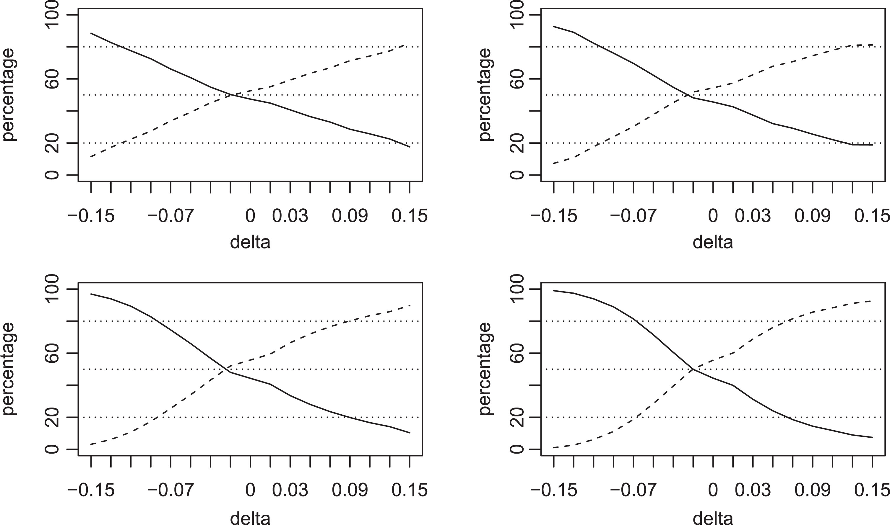
Fig. 5
Estimated probability of winning (full line) and losing (dashed line) QSP Bof5 matches for (clockwise) pA = 0.55, 0.60, 0.65, 0.70 as a function of δ = pA - pB.
The results of our simulations shed a new light in the interpretation of the negative record of Federer. Indeed, according to our analyses, his predominance of losing QSP matches is not necessarily a signal of weakness but, on the contrary, jointly to his uncommon results, can be read as an evidence of strength and superiority.
7.Discussion and conclusions
The aim of this paper was to follow-up the work of Wright etal. (2013) for a more in-depth comprehension of the quasi-Simpson paradox in tennis.
To this end, new data have been considered, measuring QSP with respect to both points and games. Results have been also analyzed jointly to those found by Wright etal. (2013) in order to assess the statistical significance of the differences.
For men players, and referring to QSP-P, our findings are fully in line with those of Wright etal. (2013) and confirm that QSP-P occurs in around 4.5% of matches. This percentage reduces to 2.15% when QSP-G is considered. Statistical LR tests for multiple equal proportions suggest that there are not significant differences – at the 5% level – in the percentage occurrence of QSP-P and QSP-G when considering different surfaces, or different kinds of tournaments, or Bof3 and Bof5 matches. Likewise, the analysis of the percentage instances of QSP-P in different sub-periods leads to accept the hypothesis of no difference, suggesting that there were no changes for this phenomenon.
For women, QSP takes place less frequently than for men: in 3.2% of matches for QSP-P and in 1.85% of times for QSP-G. These percentages are significantly lower – at the 5% level – than those for men. Moreover, differently than for men, the test for equal proportions rejects the hypothesis of no difference between Grand Slam matches and other tournaments matches, both for QSP-P and for QSP-G. This difference can be due to the different role played by the service between men and women.
QSP has been also studied through Monte Carlo simulations under the hypothesis of i.i.d. points. Results show that the statistical features of the data generating process together with the three level scoring system of tennis, is enough to explain the observed occurrences of QSP-P and QSP-G. Even the distribution of the difference of points in case of simulated QSP matches is quite similar to that empirically observed. Thus, although there is no formal evidence, our results hint that the occurrence of QSP is not due to a player’s voluntary strategy but can be considered simply as a statistical quirk of tennis’ scoring system.
As to the Federer paradox, our findings suggest that his apparently negative record can also be read, in the opposite way, as a clue of his superiority.
References
1 | Baca, A. , 2015, Computer Science in Sport: Research and Practice. Routledge. |
2 | Klaassen, F. and Magnus, J.R. , (2001) , Are points in tennis independent and identically distributed? Evidence from a dynamic binary panel data, Journal of the American Statistical Association, 96, 500–509. |
3 | Klaassen, F. and Magnus, J.R. , (2014) , Analyzing Wimbledon. The Power of Statistics. Oxford University Press. |
4 | Lawrence, A. , (2013) , Surviving the U.S. open. Sports Illustrated, 30: :September 2. |
5 | Matheson, V. , (2007) , Research note: Athletic graduation rates and Simpson’s paradox, Economics of Education Review 26: , 516–520. |
6 | Newton, P.K. and Aslam, K. , (2009) , Monte Carlo tennis: A stochastic Markov chain model, Journal of Quantitative Analysis in Sports 5, 1–44. |
7 | O’Donoghue, P. , (2013) , Rare events in tennis, International Journal of Performance Analysis in Sport 13, 535–552. |
8 | Wardrop, R.L. , (1995) , Simpson’s paradox and the hot hand in basketball, The American Statistician 49: , 24–28. |
9 | Wasserman, L. , 2004, All of Statistics: A Concise Course in Statistical Inference. Springer. |
10 | Wright, B. , Rodenberg, R.M. , and Sackmann, J. , (2013) , Incentives in best of N contests: Quasi-Simpson’s paradox in tennis, International Journal of Performance Analysis in Sports 13, 790–802. |
Notes
3 OnCourt is a piece of software including data for all matches played since 1990. For more details, see http://www.oncourt.info.
4 For example, up to October 2018, at Wimbledon, Roland Garros and Australian Open, there was not tie-break in the fifth set. In October 2018 it was introduced at Wimbledon at the score of 12 - 12.


