
Forecasting college football game outcomes using modern modeling techniques
Abstract
There are many reasons why data scientists and fans of college football would want to forecast the outcome of games – gambling, game preparation and academic research, for example. As advanced statistical methods become more readily accessible, so do the opportunities to develop robust forecasting models. Using data from the 2011 to 2014 seasons, we implemented a variety of advanced modeling techniques to determine which best forecasts the outcome of games. These methods included ridge regression, the lasso, the elastic net, neural networks, random forests, k-nearest neighbors, stochastic gradient boosting, and a Bayesian regression model. To evaluate the efficacy of the proposed models, we tested them on data from the 2015 season. The top performers – lasso regression, a Bayesian regression with team-specific variances, stochastic gradient boosting, and random forests – predicted the correct outcome over 70% of the time, and the lasso model proved most accurate at predicting win-loss outcomes in the 2015 test data set.
1Introduction
College football has become a major business unto itself. Gaul (2015) noted 10 of the larger institutions investing in the sport earned revenues of $762 million in 2012. Television contracts often value in the billions; for example, to televise the College Football Playoff for 12 years, ESPN reportedly paid $5.64 billion for the duration of the contract, per Bachman (2012). However, the academic literature concerning the prediction of college football outcomes is fairly limited. Stefani (1977) detailed how to use a least squares method to come up with rankings for all college football teams, and then determine a winner based upon which team has the better ranking. Three years later, Stefani (1980) improved upon an existing simple least squares method to rank teams weekly (i.e., not requiring the difference of rankings to equal the margin of victory) and then used the upgraded rankings to determine winners for specific games. Elo (2008) highlighted his ranking system that was originally used to compare chess players. Once it was modified to include football, he presented an equation that could be used to generate an expected probability of Team A winning a game over Team B. Delen, et al. (2012) took a slightly different approach to rankings by using data mining techniques to predict bowl games. Leung and Joseph (2014) abandoned the idea of rankings altogether by using a classification analysis to group teams, pick out two groups most similar to the competing teams in a particular game, analyze the outcomes when teams within those two groups played each other, and used that information to predict which team would win the game in question.
In this manuscript, we combine two sources of college football data – box scores and recruiting data – and apply multiple modern modeling techniques to identify the method that most accurately predicts the winner of NCAA football games. Specifically, we train a series of models using data from the 2011– 2014 seasons via ridge regression, the lasso, the elastic net, k-nearest neighbors, neural networks, gradient boosting machines, and a Bayesian hierarchical linear model. Our contribution to the literature is two-fold: first, we identify a subset of variables that are meaningful predictors of the outcomes of college football games according to the methods used. Next, we present the predictive power of the models by validating them using data from the 2015 season. To the best of our knowledge, our study is the most comprehensive with respect to the data considered in model construction and validation.
2Methodology
2.1Dataset
The data used for this research consists of 4,339 games between Football Bowl Subdivision (FBS) teams between the 2011 and 2015 seasons; the data was provided by college football database administrator Marty Coleman2 To maximize the utility of the data, several adjustments were made. First, we removed games including non-FBS opponents (e.g. FCS, Division II, etc.) as there was not complete season data for schools at that level, nor are those games (usually) representative of a traditional college football game. Next, individual game results were converted to season-long moving averages. For example, to predict the outcome for Alabama’s sixth game of the 2012 season, we used averages of their statistics for all games available prior to this (excluding games against opponents from lower classifications), as well as averages of their opponent prior to Alabama’s sixth game. For Alabama’s seventh game, we included the results from the sixth game in the moving averages, and so forth. Additionally, we hypothesized that outcomes could be related to relative differences between the teams rather than absolute performance. So, the following covariates were created: difference in offensive points scored vs. opponent defensive points allowed, difference in defensive points allowed vs. opponent offensive points scored, difference in yards per pass attempt (YPPA) between the team and opposing defense as well as the team defense and opposing offense, difference in yards per rush attempt (YPRA) between the team and opposing defense as well as the team defense and opposing offense, difference in pass yards between the team and opposing defense as well as the team defense and opposing offense, difference in rush yards between the team and opposing defense as well as the team defense and opposing offense, turnover difference, win percentage difference, difference in total offensive and defensive plays, and difference in both offensive yards and defensive yards allowed. Note that these were differences of the moving averages. Lastly, composite team rankings from 247sports.com were used to quantify the level of talent on each team. The 247 composite team rankings (2012) are generated by “a proprietary algorithm that compiles rankings and ratings listed in the public domain by the major media recruiting services.” The recruiting classes for each school each receive an annual composite score based upon how other recruiting services ranked the group as a whole. Because college players have four years of eligibility, the four classes preceding the year of the games will capture the quality of talent playing in a specific game. This study includes all class rankings dating back to 2008, so that freshmen from the 2008 class (becoming true seniors in 2011) can be represented in the dataset. Because it often takes talent some time to develop – especially at well-established schools – we included four lags of composite rankings, as well as averages of the previous two, three, and four annual composite rankings. Lastly, in college football, home field advantage has been found to be an important consideration. Moskowitz and Wertheim (2011) studied nineteen different sports at varying levels spanning more than forty countries. In college football, they discovered that 64.1% of all home teams won, ranking sixth among the nineteen sports studied. They also found that, “in 140 seasons of college football, there has never been a year when home teams have failed to win more games than road teams.” (p. 113). Fair and Oster (2007) estimated the home field advantage in college football to be between 4.1 and 4.7 points. Given this information and the fact that there are three possible locations – home, away, and neutral – we created a “field status” variable that gives equal weight to home and away status: a value of 1 was assigned for all home games, 0 for neutral, and – 1 for away games. In total, 83 candidate predictors were available3. The outcome variable was chosen to be the difference in point total, as it retains more information about the matchup compared to a binary “win” or “loss.”
2.2Models Considered
In terms of modeling frameworks, we selected the following:
– Ridge Regression
– Least absolute shrinkage and selection operator (lasso)
– Elastic Net
– Neural Network
– Random Forests
– K-Nearest Neighbors
– Bayesian Linear Model with Team Specific Variances
A high-level overview of most of these frameworks can be found in James et al. (2013), among other sources. Ridge regression, as explained by Hoerl and Kennard (1970) is a linear model, but instead of calculating coefficients by minimizing the residual sum of squares as in ordinary least squares regression, a penalty term is added based on the L2 norm of the regression parameters, causing shrinkage. The primary benefit is that it reduces the variance introduced by correlated predictors, at the expense of introducing bias in the form of a penalty term (with the hope of reducing the overall mean squared error). Tibshirani (1996) explained the least absolute shrinkage and selection operator (lasso) is similar to ridge regression with the exception that it penalizes the L1 norm of the regression parameters. This penalty has the added benefit of shrinking some of the regression parameters to zero, functioning as a variable selection technique. This feature is especially useful given the large number of variables in the data set and uncertain utility of many of them. Ridge regression and the lasso can be thought of as being on opposite ends of the spectrum – the ridge penalty shrinks parameter estimates but keeps them all in the model, while the lasso shrinks some to exactly zero (with the number of non-zero coefficients decreasing as the penalty increases). A further extension of ridge regression and lasso regression was developed by Zou and Hastie (2005), who present elastic net regression as a function of the two, with a second tuning parameter introduced to control the degree to which the model moves closer to ridge regression or lasso regression. An additional benefit is the elastic net tends to select correlated variables together, keeping them either in or out of the model, while lasso regression tends to select one arbitrarily. These three methods were implemented in R (2016) using the glmnet package written by Friedman, Hastie and Tibshirani (2010), with all tuning and penalty parameters chosen via repeated 10-fold cross-validation within the caret package, written by Kuhn (2008).
The neural network – a non-parametric model – was described by Günther and Fritsch (2010) as being based upon the makeup of the human brain, where electrical signals are transmitted to different neurons through axons and dendrites and received by synapses. In application, attributes of a dataset go into the model through the use of input nodes. As it passes through to the hidden layer(s), assigned weights adjust the importance of the input (the higher the weight, the greater the importance). Once it passes through the necessary hidden layers, it reaches an output layer representing a target value. In this study, the output is the projected point difference between two teams and the hidden layers are constructed from combinations of the different variables in the dataset. Collinearity can cause computational problems in this modeling paradigm, so pairs of highly correlated predictors were identified (in this case, with r > 0.75) and, amongst the pairs, the predictors with the largest mean absolute correlation with the remaining predictors was removed. We fit a neural network using the nnet package in R from Günther and Fritsch (2016) by tuning the number of hidden units and the weight decay, and then determining whether bagging improved the model fit. Breiman (2001) explained how random forests are generated from another non-parametric algorithm that relies on bootstrapping and random sampling of predictors to build a series of decision trees, and then uses the average of the individual predictions as the overall ensemble prediction. They were fit using the randomForest package in R from Liaw and Wiener (2002), with the number of randomly selected predictors as the only tuning parameter. The k-nearest neighbors (KNN) approach, explained by Altman (1992), uses Euclidean distances to identify which observations are nearest in proximity, and then uses the mean of the outcome for the neighbors as its prediction; this was done via the FNN package in R by Beygelzimer et al. (2013) with the number of neighbors as the only tuning parameter. Friedman (2001) discusses gradient boosting, a tool that has recently gained lots of traction in the machine learning community. This technique optimizes an objective function that is a combination of a loss function and a regularization function, with the general principle being to define a parsimonious but predictive model. It iteratively builds an ensemble of decision trees that – while individually are not strong predictors – become strong when taken together. The xgboost package by Chen et al. (2017) is highly customizable and is often used in big data competitions4 Tree boosting functions were used, with the following tuning parameters: max tree depth, percentage of columns sampled, percentage of rows sampled, the number of rounds, minimum child weight, and eta. The caret package was used to select the tuning parameters here, as well as for the neural network and random forest.
The Bayesian framework was the last major modeling paradigm considered. Similar to South et al. (2017), we use a linear model to predict the outcome, but in this case allowed for team-specific precisions (note that a model with team-specific regression coefficients was also tested, but is not reported as it was inferior to the model presented below). The model specification is as follows:
A combination of R and WinBUGS (Lunn et al. (2000)) were used to fit the model. Note that WinBUGS uses precision (the inverse of variance) in the specification of a normal distribution, which explains the use of the precision parameter rather than the standard deviation in the presented model specifications. Also note that conventional non-informative priors were assigned to the parameters.
One additional challenge in the analysis was introduced due to the necessity of including statistics related to opponent strength. For example, in instances where SMU played Houston, the decision had to be made whether to call SMU the “team” and Houston the “opponent,” or vice versa. The most unbiased way to address this was via random chance, and this was the approach taken for each game in the data set. While this did introduce an extra source of variability (via the random selection process), it allowed for the estimation of the effect of the field status parameter as discussed in Section 2.1. Further, in the modern era of college football, it is common for teams to pay lesser opponents to play road games at their venues, meaning the home/away status of a game is not necessarily independent of team quality5 The models were trained and validated after taking this approach, but to understand the implications of the random assignment of “team” and “opponent,” we repeated the random assignment process a total of 50 times. To minimize the computational burden, the initial tuning parameters (chosen from the first random assignment) were retained and the models were re-fit according to these parameters. The subsequent root mean squared errors from the validation sets were stored, allowing for an analysis of variance (with post-hoc comparisons) to explore whether there was any separation between the methods. Lastly, the predicted outcomes for the top performing models were converted using a decision rule – a positive value indicated a predicted victory for the team over their opponent, and a negative value indicated the opposite; this was done to give a more intuitive measure of model strength.
3Results
3.1Features retained using penalized regression
The repeated 10-fold cross validation found that lasso regression was a better predictive framework than the elastic net or ridge regression. Table 1 lists the 26 variables retained by lasso regression (recall that, aside from the field status variable, they are all average measures up to the point in the season of the corresponding observation).
Table 1
Lasso selected variables
| Rushing Attempts | Yards Per Rush Attempt (YPRA) | Total Yards | Yards Per Play (YPP) |
| Turnovers Committed (TO) | Penalty Yards Accrued | Pass Attempts Against | YPRA Allowed |
| Turnovers Forced | Point Differential | Opponent Offense Pass Yards | Opponent Offense Yards Per Play |
| Opponent Offense Penalty Yards | Opponent Defense YPPA | Opponent Defense Rush Yards Allowed | Opponent Defense Total Yards Allowed |
| Opponent Defense Yards Per Play Allowed | Opponent Turnovers Forced | Opponent Defense Penalty Yards Accrued | Opponent Point Differential |
| Difference in Team and Opponent Win Percentage | Composite Ranking (CR), Lag 2 | Average CR (Last 2 Years) | Average CR (Last 3 Years) |
| Average CR (Last 4 Years) | Field Status |
Knowledgeable college football fans will note the selected variables are quite reasonable, as game location, measures of offensive volume and efficiency (YPRA, total yards, YPP, point differential), defensive volume (rushing yards allowed, total yards allowed), opponent offensive volume and efficiency (rushing attempts, yards per play, point differential), opponent defensive volume and efficiency (passes faced, YPRA allowed, total yards allowed, yards per play allowed, turnovers forced), difference in win percentage and team talent were all predictive of outcome. Additionally, the signs of the regression coefficients also matched with intuition – for example, increases in team offensive metrics (such as total yards gained) and opponent defensive metrics (such as YPRA allowed) led to an increase in the expected point differential, while increases in team defensive metrics (such as rushing yards allowed) or opponent offensive metrics (such as yards per play) lowered the expected point differential.
Figure 1 displays the variables according to their importance, calculated via the varImp function from the caret package. The bars have also been colored by the sign of the parameter estimates. For example, as the gap in win percentage between the team and its opponent increases, so does the estimated point differential (in favor of the team); contrastingly, as the opponent offense’s YPP increase, the expected point differential decreases.
Fig. 1
Variable importance, Lasso selected variables
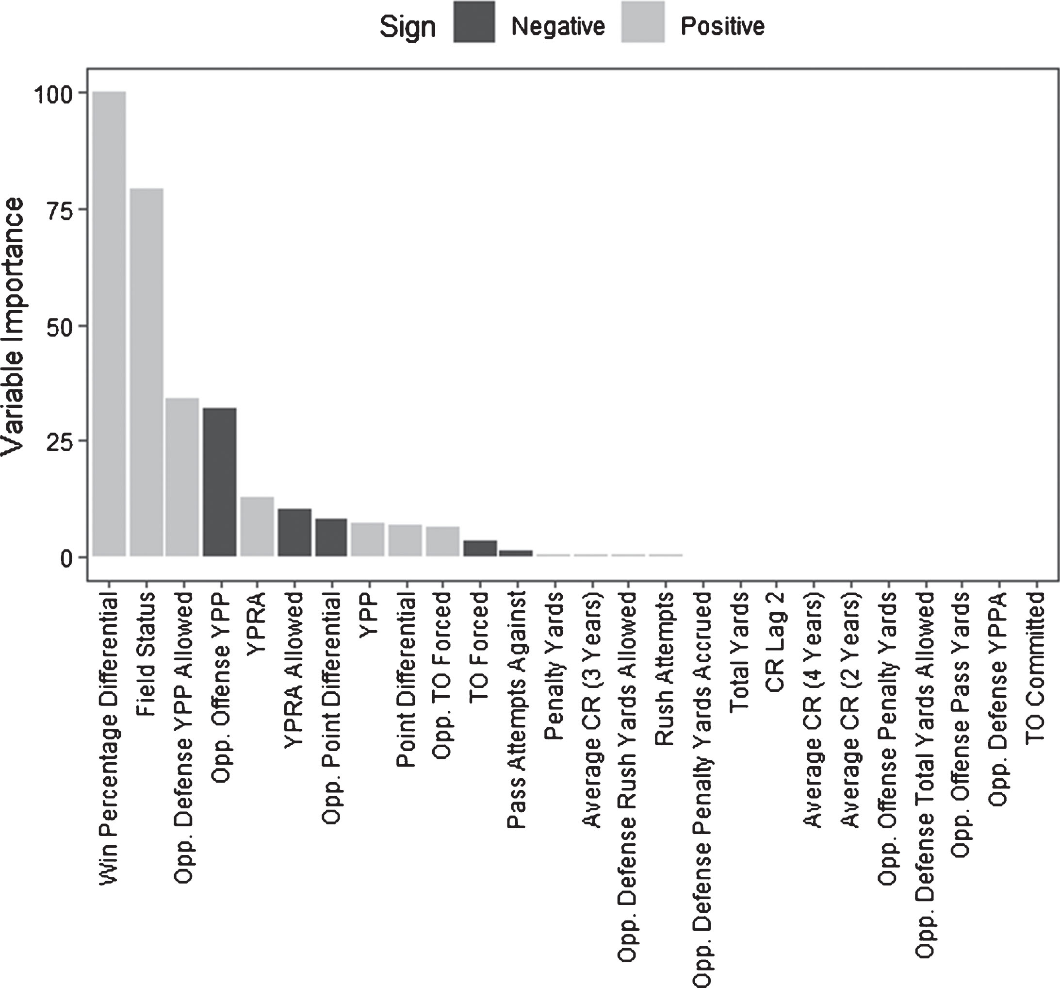
From this, it is clear that though 26 variables were selected by the lasso, the efficacy of the model is driven by only a few of them – notably the difference in team strength, location of the game, and overall opponent offensive and defensive strength. We note that the estimated lasso regression coefficients for field status was 3.6, implying a swing of over a touchdown advantage when playing at home versus playing away, after controlling for the other metrics in Table 1.
Though the “black box” approaches (KNN, neural networks, gradient boosting, and random forests) do not give specific information about the magnitude or direction of the predictors, a variable importance metric is still available via the caret package. The most important variables according to this metric were consistently the difference in win percentage between the team and current opponent, average point differential for the current opponent, average point differential for the team, and location – seeming to agree with the types of variables selected by the lasso regression.
3.2Model evaluation
For parsimony, the retained variables from the lasso regression were those used in the Bayesian model. For the neural network, predictors whose pairwise correlation coefficient exceeded 0.75 were identified, and the predictor with the largest mean absolute correlation relative to all other predictors was removed. This process was carried out using the findCorrelation function from the caret package. The other modeling approaches utilized all available predictors. After training each model on the 2011– 14 data, data from the 2015 season was used as a test data set. Table 2 gives the average root mean squared error across the 50 random assignments of “Team” and “Opponent,” as well as the overall prediction rate according to the first random assignment.
Table 2
Forecasting success rates for each modeling paradigm (2015 season)
| Model | Mean RMSE (SD) | Overall Prediction |
| Lasso | 17.00 (0.08) | 75.0% |
| Random forest | 17.00 (0.11) | 72.9% |
| K-nearest neighbors | 17.73 (0.10) | 70.7% |
| Neural network | 17.37 (0.18) | 69.7% |
| Bayesian linear model | 17.02 (0.12) | 72.2% |
| Gradient boosting | 17.02 (0.15) | 71.7% |
RMSE=Root mean squared error, SD = standard deviation
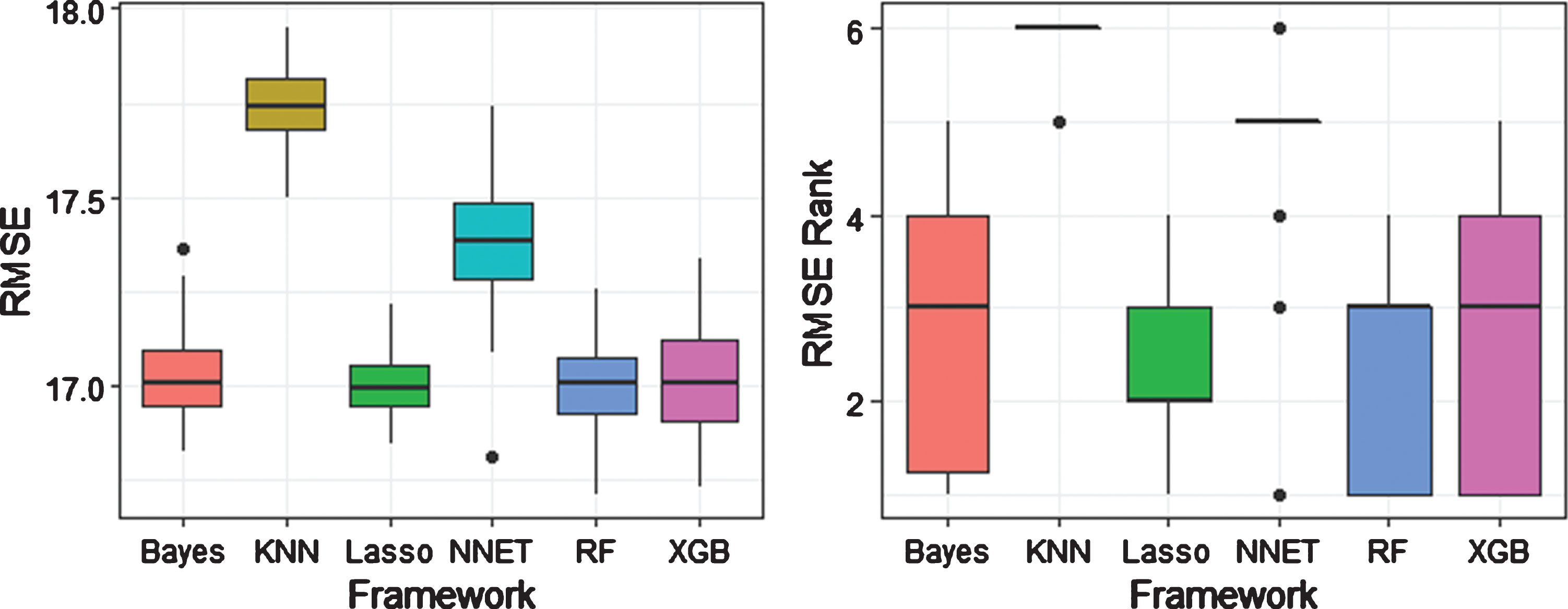
An analysis of variance with Tukey’s post-hoc comparisons found that lasso regression, the random forest, the Bayesian linear model, and the XGBoost model were superior to the other three methods, but were not significantly different from each other (p ≈ 1 for all three comparisons). Figure 2 displays boxplots of the results from the random assignments, both by RMSE and RMSE rank. The lasso had the least variability among the competing methods in terms of RMSE, but it was only the top ranked method in 5 of the 50 repetitions, while random forests and XGBoost were first 16 and 15 times, respectively. However, the lasso was also able to correctly identify the largest percentage of outcomes in the test data set when using a simple decision rule.
Fig. 2
Competing model root mean squared error (RMSE) and RMSE rank from 50 random assignments of “Team” and “Opponent”
4Conclusion
The results of this study are promising. Beginning with a large set of variables that included offensive and defensive characteristics, relative strength, and talent metrics, we were able to identify a subset that contained information to predict the outcome of NCAA football games. We did a survey of linear, non-parametric and Bayesian methods, and found that lasso regression, random forests, a Bayesian linear model with team-specific precisions, and stochastic gradient boosting via XGBoost were the most efficacious models in terms of root mean squared error, and were able to successful predict over 70% of outcomes from the 2015 season (bowl games included) using a model built on data from the 2011– 2014 seasons. Though these methods were statistically inseparable, due to it having the lowest variability among RMSE values and top binary outcome predictive value (as well as the interpretability of model coefficients), the authors lean towards recommending the lasso as the method of choice; however, arguments could be made for the other modeling paradigms as well. As with any study, there are a number of limitations. First, this manuscript does not present an exhaustive search of advanced statistical methods, nor do we propose any new unique methodology. In particular, state space models (Glickman and Stern, 1998 & Lopez, Matthews, and Baumer, 2017, among others) based on the Bradley-Terry model of paired comparisons (Bradley and Terry, 1952) would be expected to perform similarly to some of the approaches in this paper. We also did not do an exhaustive search of the vast array of tuning parameters available to some of the machine learning techniques (gradient boosting in particular). Further, we chose to model the point difference as the outcome rather than the binary win/loss result; had we chosen to use a general linear model framework we may have observed different results. Nonetheless, the authors hope that these results lead researchers to further develop and publish in the field of predictive analytics for college football – an area in which most approaches are proprietary given the prospect for financial or reputation gain.
Table 3
Variables in college football dataset
| Name | Description (all averages are season-specific) |
| Team Points | Average number of points scored |
| Team Passes | Average number of passes thrown |
| Team Passing Yards | Average number of passing yards |
| Team YPPA | Average number of yards per passing attempt |
| Team Rush Attempts | Average number of rushing attempts |
| Team Rush Yards | Average number of rush yards |
| Team YPRA | Average number of yards per rushing attempt |
| Team Total Plays | Average number of offensive plays |
| Team Total Yards | Average number of total yards gained on offense |
| Team YPP | Average number of yards gained per play |
| Team TO | Average number of turnovers (giveaways) |
| Team Penalty Yards | Average number of penalty yards accumulated by the team |
| Team TOP | Average offensive time of possession (in seconds) |
| Opponent Points | Average number of points allowed by the team’s defense |
| Opponent Passes | Average number of passes faced by the team’s defense |
| Opponent Passing Yards | Average number of passing yards allowed by the team’s defense |
| Opponent YPPA | Average number of yards per passing attempt allowed by the team’s defense |
| Opponent Rush Attempts | Average number of rushing attempts allowed by the team’s defense |
| Opponent Rush Yards | Average number of rushing yards allowed by the team’s defense |
| Opponent YPRA | Average number of rushing yards per attempt allowed by the team’s defense |
| Opponent Total Plays | Average number of offensive plays faced by the team’s defense |
| Opponent Total Yards | Average number of total yards allowed by the team’s defense |
| Opponent YPP | Average number of yards per play allowed by the team’s defense |
| Opponent TO | Average number of turnovers forced (takeaways) by the team’s defense |
| Opponent Penalty Yards | Average number of penalty yards accrued by team’s opponents |
| Opponent Time of Possession | Average time of possession allowed by the team’s defense |
| Victory | Average win percentage for the team |
| Points Differential | Average point differential for the team |
| TO Difference | Average turnover differential (takeaways-giveaways) for the team |
| Opponent Offensive Points | Average points scored by the current opponent |
| Opponent Offensive Passes | Average number of passes by the current opponent’s offense |
| Opponent Offensive Pass Yards | Average number of passing yards gained by the current opponent’s offense |
| Opponent Offense YPPA | Average yards per pass attempt gained by the current opponent’s offense |
| Opponent Offense Rush Attempts | Average number of rush attempts by the current opponent’s offense |
| Opponent Offense Rush Yards | Average number of rush yards gained by the current opponent’s offense |
| Opponent Offense YPRA | Average number of rush yards per play gained by the current opponent’s offense |
| Opponent Offense Total Plays | Average number of total plays by the current opponent’s offense |
| Opponent Offense Total Yards | Average number of total yards gained by the current opponent’s offense |
| Opponent Offense YPP | Average number of yards per play gained by the current opponent’s offense |
| Opponent Offense TO | Average number of turnovers committed by the current opponent |
| Opponent Offense Penalty Yards | Average number of penalty yards accrued by current opponent |
| Opponent Offense TOP | Average time of possession by the current opponent’s offense |
| Opponent Defense Points | Average number of points given up by the defense of the current opponent |
| Opponent Defense Passes | Average number of passes faced by the defense of the current opponent |
| Opponent Defense Pass Yards | Average number of passes yards allowed by the defense of the current opponent |
| Opponent Defense YPPA | Average yards per pass attempt given up by the defense of the current opponent |
| Opponent Defense Rush Attempts | Average number of rush attempts faced by the defense of the current opponent |
| Opponent Defense Rush Yards | Average number of rush yards given up by the defense of the current opponent |
| Opponent Defense YPRA | Average number of rush yards per attempt given up by the defense of the current opponent |
| Opponent Defense Total Plays | Average number of total plays faced by the defense of the current opponent |
| Opponent Defense Total Yards | Average number of yards allowed by the defense of the current opponent |
| Opponent Defense YPP | Average number of yards per play allowed by the defense of the current opponent |
| Opponent Defense TO | Average number of turnovers forced (takeaways) by the defense of the current opponent |
| Opponent Defense Penalty Yards | Average number of penalty yards accrued by opponents of the current opponent |
| Opponent Victory | Win percentage of the current opponent |
| Opponent Point Differential | Average point differential of the current opponent |
| Opponent TO Diff | Difference in the average turnovers forced (takeaways) and committed (giveaways) by the current opponent |
| Offense Points Diff | Difference in the average points scored by the team and average points allowed by the current opponent’s defense |
| Defense Points Diff | Difference in the average points scored by the current opponent and the average points allowed by the team’s defense |
| Offense YPPA Diff | Difference in the average yards per pass attempt by the team’s offense and the average yards per pass attempt allowed by the current opponent’s defense |
| Defense YPPA Diff | Difference in the average yards per pass attempt allowed by the team’s defense and the average yards per pass attempt by the current opponent’s offense |
| Offense YPRA Diff | Difference in the average yards per rush attempt by the team’s offense and the average yards per rush attempt allowed by the current opponent’s defense |
| Defense YPRA Diff | Difference in the average yards per rush attempt allowed by the team’s defense and the average yards per rush attempt by the current opponent’s offense |
| Offense Pass Yards Diff | Difference in the average total passing yards gained by the team’s offense and the average passing yards allowed by the current opponent’s defense |
| Defense Pass Yards Diff | Difference in the average total passing yards allowed by the team’s defense and the average passing yards gained by the current opponent’s offense |
| Offense Rush Yards Diff | Difference in the average total rushing yards gained by the team’s offense and the average rushing yards allowed by the current opponent’s defense |
| Defense Rush Yards Diff | Difference in the average total rushing yards allowed by the team’s defense and the average rushing yards gained by the current opponent’s offense |
| TO Diff Diff | Difference in the average turnover differential between the team and current opponent |
| Victory Diff | Difference in win percentage between the team and current opponent |
| Offense Total Plays Diff | Difference in average total plays by the team’s offense and the average total plays faced by the defense of the current opponent |
| Defense Total Plays Diff | Difference in the average total plays faced by the team’s defense and the average total plays by the offense of the current opponent |
| Offense Total Yards Diff | Difference in average total yards gained by the team’s offense and the average total yards allowed by the defense of the current opponent |
| Defense Total Yards Diff | Difference in the average total yards gained by the team’s defense and the average total yards allowed by the offense of the current opponent |
| Home Indicator | Whether or not the team was home (1 = yes, 0 = no) |
| Away Indicator | Whether or not the team was away (1 = yes, 0 = no) |
| Recruit Lag 1 | The average 247 composite ranking from the team’s prior recruiting class |
| Recruit Lag 2 | The average 247 composite ranking from the team’s recruiting class 2 seasons ago |
| Recruit Lag 3 | The average 247 composite ranking from the team’s recruiting class 3 seasons ago |
| Recruit Lag 4 | The average 247 composite ranking from the team’s recruiting class 4 seasons ago |
| Recruit Average 2 | The average of the 247 composite ranking from the team’s 2 previous recruiting classes |
| Recruit Average 3 | The average of the 247 composite ranking from the team’s 3 previous recruiting classes |
| Recruit Average 4 | The average of the 247 composite ranking from the team’s 4 previous recruiting classes |
Acknowledgments
The authors wish to thank Mr. Shen and the two anonymous reviewers for their constructive feedback and suggestions that resulted in a more comprehensive, sound paper.
References
1 | 247Sports Staff., 2012. 247Sports Rating Explanation. [online] Available at: http://247sports.com/Article/247Rating-Explanation-81574 [Accessed 14 Dec. 2019] |
2 | Altman N.S. , (1992) . An introduction to kernel and nearest-neighbor nonparametric regression, The American Statistician 46: (3), 175–185. |
3 | Bachman R. , 2012. ESPN Strikes Deal for College Football Playoff. [online] Available at: https://www.wsj.com/articles/SB10001424127887324851704578133223970790516 [Accessed 14 Dec. 2019] |
4 | Beygelzimer A. , Kakadet S. , Langford J. , Arya S. , Mount D. and Li S. , (2013) . FNN: Fast nearest neighbor search algorithms and applications, R package version 1: (1). |
5 | Bradley R.A. and Terry M.E. , (1952) . Rank analysis of incomplete block designs: I. The method of paired comparisons, Biometrika 39: (3/4), 324–345. |
6 | Breiman L. , (2001) . Random forests, Machine learning 45: (1), pp. 5–32. |
7 | Chen T. , He T. , Benesty M. , Khotilovich V. and Tang Y. , (2015) . Xgboost: Extreme gradient boosting, Rpackage version 0.4-2. 1–4. |
8 | Delen D. , Cogdell D. and Kasap N. , (2012) . A comparative analysis of data mining methods in predicting NCAA bowl outcomes, International Journal of Forecasting 28: (2), 543–552. |
9 | Friedman J.H. , (2001) . Greedy function approximation: a gradient boosting machine, Annals of statistics pp. 1189–1232. |
10 | Fair R.C. and Oster J.F. , (2007) . College football rankings and market efficiency, Journal of Sports Economics 8: (1), 3–18. |
11 | Friedman J. , Hastie T. and Tibshirani R. , (2010) . Regularization paths for generalized linear models via coordinate descent, Journal of statistical software 33: (1), 1. |
12 | Gaul G.M. , (2015) . Billion-dollar ball: A journey through the big-money culture of college football, Penguin. |
13 | Glickman M.E. and Stern H.S. , (1998) . A state-space model for National Football League scores, Journal of the American Statistical Association 93: (441), 25–35. |
14 | Günther F. and Fritsch S. , (2010) . neuralnet: Training of neural networks, The R journal 2: (1), 30–38. |
15 | Hoerl A.E. and Kennard R.W. , (1970) . Ridge regression: Biased estimation for nonorthogonal problems, Technometrics 12: (1), 55–67. |
16 | James G. , Witten D. , Hastie T. and Tibshirani R. , (2013) . An introduction to statistical learning (Vol. 112, p. 18). New York: springer. |
17 | Kuhn M. , (2008) . Building predictive models in R using the caret package, Journal of statistical software 28: (5), 1–26. |
18 | Leung C.K. and Joseph K.W. , (2014) . Sports data mining: predicting results for the college football games, Procedia Computer Science 35: , 710–719. |
19 | Liaw A. and Wiener M. , (2002) . Classification and regression by randomForest, R news 2: (3), 18–22. |
20 | Lopez M.J. , Matthews G.J. and Baumer B.S. , (2018) . How often does the best team win? A unified approach to understanding randomness in North American sport, The Annals of Applied Statistics 12: (4), 2483–2516. |
21 | Lunn D.J. , Thomas A. , Best N. and Spiegelhalter D. , (2000) . WinBUGS-a Bayesian modelling framework: concepts, structure, and extensibility, Statistics and computing 10: (4), 325–337. |
22 | Moskowitz T. and Wertheim L.J. , (2012) . Scorecasting: The hidden influences behind how sports are played and games are won, Three Rivers Press (CA). |
23 | Team R.C. , (2016) . A language and environment for statistical computing. R Foundation for Statistical Computing, Vienna, Austria, version 3.3. 0. URL Available: https://www.R-project.org/ (Accessed October 2017). |
24 | South C. , Elmore R. , Clarage A. , Sickorez R. and Cao J. , (2019) . A Starting Point for Navigating the World of Daily Fantasy Basketball, The American Statistician 73: (2), 179–185. |
25 | Stefani R.T. , (1977) . Football and basketball predictions using least squares, IEEE Transactions on systems, man, and cybernetics 7: (2), 117–21. |
26 | Stefani R.T. , (1980) . Improved least squares football, basketball, and soccer predictions, IEEE Transactions on systems, man, and cybernetics 10: (2), 116–123. |
27 | Tibshirani R. , (1996) . Regression shrinkage and selection via the lasso, Journal of the Royal Statistical Society: Series B (Methodological) 58: (1), 267–288 |
28 | Zou H. and Hastie T. , (2005) . Regularization and variable selection via the elastic net, Journal of the royal statistical society: series B (statistical methodology) 67: (2), 301–320. |
Notes
2 His data can be found on his website: http://www.seldomusedreserve.com/?page_id=8805.
3 A full list is given in the appendix.


