
Empirical study on relationship between sports analytics and success in regular season and postseason in Major League Baseball
Abstract
In this paper, we study the relationship between sports analytics and success in regular season and postseason in Major League Baseball via the empirical data of 2014-2017. The categories of analytics belief, the number of analytics staff, and the total number of research staff employed by MLB teams are examined. Conditional probabilities, correlations, and various regression models are used to analyze the data. It is shown that the use of sports analytics might have some positive impact on the success of teams in the regular season, but not in the postseason. After taking into account the team payroll, we apply partial correlations and partial F tests to analyze the data again. It is found that the use of sports analytics, with team payroll already in the regression model, might still be a good indicator of success in the regular season, but not in the postseason. Moreover, it is shown that both the team payroll and the use of sports analytics are not good indicators of success in the postseason. The predictive modeling of decision trees is also developed, under different kinds of input and target variables, to classify MLB teams into no playoffs or playoffs. It is interesting to note that 87 wins (or 0.537 winning percentage) in a regular season may well be the threshold of advancing into the postseason.
1Introduction
In recent years, sports analytics has been very popular in professional baseball teams among other professional sports in North America. The movie “Money Ball” vividly portrayed a true story of the magical use of sabermetrics. A team under financial constraint in Major League Baseball (MLB) was formed. Nevertheless, it thrived and successfully competed with high payroll teams in the league. Many baseball management teams nowadays have allocated plenty of financial resources to sports analytics in order to improve teams’ performance. In particular, they wish to analyze the statistics of their players and those of other teams’ players to devise more strategic game plans to give their team advantages of winning games. One could argue that the sports analytics belief in a team is an indicator of management style or management quality. One would then hypothesize that greater management quality, all else being equal, translates into more wins and hence greater success in both regular season and postseason. One might even desire that this eventually leads to winning a championship of the professional sport. But some management teams do not believe in the notion of sports analytics at all. They still utilize the traditional methods to set up game plans, using their professional knowledge and experience to guide their decisions rather than taking full advantage of the statistics of all players. Other management teams, however, are skeptical or gradually buy in the idea of sports analytics.
In this paper, we study the relationship between sports analytics and the performance of MLB teams. In particular, we look at the final standings of both regular season and postseason of 2014-2017. To assess the use of sports analytics in MLB teams, we will examine three aspects. The first aspect comes from a source outside of the teams, which is the ESPN sports analytics categorization of teams listed in The Great Analytics Rankings (2015). The sports analytics belief in MLB teams was categorized in five levels: All-in, Believers, One-foot-in, Skeptics, and Non-believers. The second and third aspects come from the source inside of the teams. We look at the number of analytics staff hired and devoted to the analytics department, if any, of each team. In addition, we investigate the total number of research staff worked in the baseball operations of each team. The research work may include analytics, statistical data analysis, mathematical modeling, data science, data architecture, decision sciences, informatics, performance science, research and development, etc. The categories of analytics belief and these numbers of analytics staff and research staff might reflect teams’ commitment and their potential shift into more reliance on analytics and other innovative research. We will evaluate how the use of sports analytics influences the number of games won in the regular season, thereby affecting the chances of advancing to the postseason. Once a team is in postseason, we will study further how the use of sports analytics influences its chances of getting into the last 4 teams and last 2 teams of playoffs, and eventually its chances of winning the championship of World Series.
Through the historical data from 1977 to 2008, Schwartz and Zarrow (2009) showed that the team payroll had great influence in regular season, but not in postseason. They also tested several other potential indicators of postseason success and found that none of them was a significant predictor. They concluded that the success in October (i.e., playoffs) was a truly random event.
It makes sense to see that teams of high payroll in general would perform better than teams of low payroll. Teams of high payroll could afford to recruit more talented and experienced players that lead to better chances of winning games. In other words, team payroll could be an indicator of the quality of players’ talent, which is an input into producing wins and success in both regular season and postseason. To confirm this belief, we will calculate the Pearson sample correlation coefficients between the success of teams and their team payroll for both regular season and postseason of 2014-2017. The Pearson sample correlation coefficients between the success of teams and their use of sports analytics are calculated as well. These results are shown in Section 3.
Binary logistic regression models and multiple linear regression models are applied to test the significance of the levels of sports analytics on the success in regular season, while ordinal logistic regression models are applied to test the significance of the levels of sports analytics on the success in postseason. The findings are also given in Section 3.
In addition to the factor of team payroll, does the use of sports analytics play an important role in explaining the success of a team (in terms of winning more games in regular season and the advancement level in postseason towards a championship of World Series)? We will tackle this issue from two perspectives. First, as the team payroll is an essential component of a team’s success, it is necessary to control this factor while calculating the correlation coefficient. Therefore, we have to calculate the partial correlation coefficient between the success of a team and its use of sports analytics, after the team payroll is accounted for. Second, we will use the partial F tests to evaluate the significance of adding the use of sports analytics in explaining the success of a team, after the factor of team payroll is already in the regression model. Moreover, we apply the model utility F test to show that both the team payroll and the use of sports analytics are not good indicators of success in the postseason. These results are shown in Section 4.
In Section 5, the predictive modeling of decision trees will be developed to classify MLB teams into no playoffs or playoffs. We will consider the situations where the number of games won in a regular season is available or not as an input variable. It is interesting to note that 87 wins (or 0.537 winning percentage) in a regular season may well be the threshold of advancing into the postseason. A decision tree shows that teams with pitchers’ salary at least $29.7 million and analytics belief either All_in or Believers have significantly higher chances of advancing to playoffs. Summary and concluding comments will be presented in Section 6.
2Data
The MLB teams’ categories of analytics belief are listed in The Great Analytics Rankings. The standings, playoffs and payrolls of the MLB teams in 2014-2017 can be found from the corresponding websites shown on the references. The numbers of analytics staff employed by teams can be tracked down from the Baseball America Directories (2014-2017). The total numbers of research staff can also be tracked down and added up from the Baseball America Directories.
3Effects of sports analytics on regular season and postseason
The MLB teams’ analytics belief can be classified in five levels (or categories) as mentioned previously. To simplify the study of conditional probabilities below, we place the levels of sports analytics belief into two groups: BELIEVERS (All-in, Believers) and NON-BELIEVERS (One-foot-in, Skeptics, Non-believers). There are 16 teams identified as BELIEVERS and the other 14 teams as NON-BELIEVERS.
3.1Conditional probabilities
3.1.1BELIEVERS/NON-BELIEVERS
The last four teams in the postseason of 2014-2017, respectively, were Baltimore Orioles (BELIEVER), St. Louis Cardinals(BELIEVER), Kansas City Royals(BELIEVER, advanced to World Series), and San Francisco(NON-BELIEVER, the champion of World Series); Chicago Cubs(BELIEVER), Toronto Blue Jays(BELIEVER), New York Mets(BELIEVER, advanced to World Series), and Kansas City Royals(BELIEVER, the champion of World Series); Los Angeles Dodgers(BELIEVER), Toronto Blue Jays(BELIEVER), Cleveland Indians(BELIEVER, advanced to World Series), and Chicago Cubs (BELIEVER, the champion of World Series); Chicago Cubs(BELIEVER), New York Yankees(BELIEVER), Los Angeles Dodgers(BELIEVER, advanced to World Series), and Houston Astros(BELIEVER, the champion of World Series). The distribution of BELIEVERS and NON-BELIEVERS teams in no playoffs and playoffs for 2014-2017 is displayed in Fig. 1.
Fig. 1.
Distribution of BELIEVERS and NON-BELIEVERS teams in no playoffs and playoffs for 2014-2017.
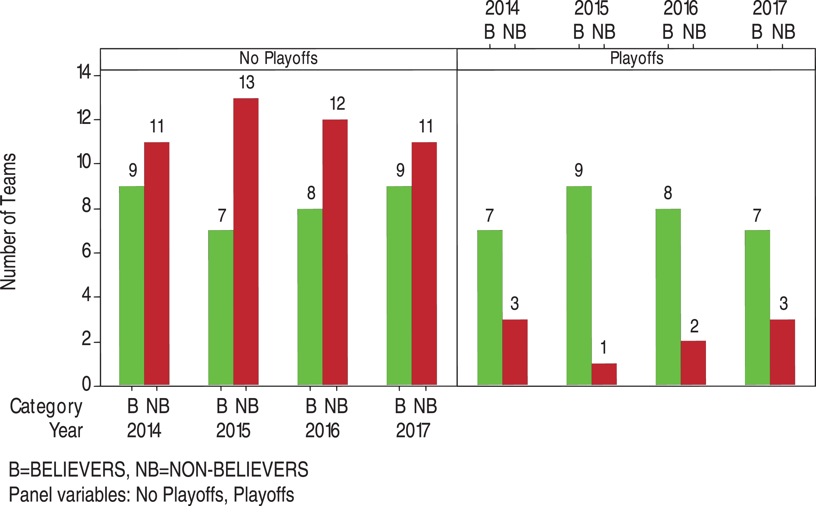
Based on Fig. 1, the conditional probabilities below show the chances of getting into playoffs if the team is a BELIEVER or a NON-BELIEVER. Once the team is in playoffs, the conditional probabilities show its chances of advancing to different stages of playoffs. The entries in the parentheses are the corresponding conditional probabilities occurred in 2014-2017.
P(Playoffs | BELIEVERS) ≈ (44%, 56%, 50%, 44%)
P(Playoffs | NON-BELIEVERS) ≈ (21%, 7%, 14%, 21%)
P(Last 4 teams of playoffs | BELIEVERS and playoffs) ≈ (43%, 44%, 50%, 57%)
P(Last 4 teams of playoffs | NON-BELIEVERS and playoffs) ≈ (33%, 0%, 0%, 0%)
P(Last 2 teams of playoffs | BELIEVERS and playoffs) ≈ (14%, 22%, 25%, 29%)
P(Last 2 teams of playoffs | NON-BELIEVERS and playoffs) ≈ (33%, 0%, 0%, 0%)
P(Champion of World Series | BELIEVERS and playoffs) ≈ (0%, 11%, 13%, 14%)
P(Champion of World Series | NON-BELIEVERS and playoffs) ≈ (33%, 0%, 0%, 0%)
Through the data of 2014-2017, we can see that the chances (44%, 56%, 50%, 44%) of advancing to playoffs for a BELIEVER team were higher than those (21%, 7%, 14%, 21%) for a NON-BELIEVER team. Once the team was in playoffs, the chances (43%, 44%, 50%, 57%) of advancing to the last 4 teams of playoffs for a BELIEVER team were also higher than those (33%, 0%, 0%, 0%) for a NON-BELIEVER team. Similar patterns remain for the data of 2015-2017, when comparing a BELIEVER team and a NON-BELIEVER team for advancing to the last 2 teams of playoffs and for becoming the champion of World Series. The data of 2014, however, shows the opposite pattern that a NON-BELIEVER team had a higher chance of advancing to the last 2 teams of playoffs than a BELIEVER team (33% vs 14%) and had a higher chance of becoming the champion of World Series (33% vs 0%). This happened because of the fact that the champion of World Series in 2014 was San Francisco which was categorized as a NON-BELIEVER team.
To test the relationship between a team’s category of analytics belief (BELIEVER or NON-BELIEVER) and whether it advances to the postseason, we apply the chi-square test for testing the independence of these two characteristics. We obtain the observed chi-square value = 1.674, 8.105, 4.286, 1.674 and p-value = 0.196, 0.004, 0.038, 0.196 for 2014-2017, respectively. Notice that both p-values for 2014 and 2017 are 0.196. Therefore, with 5% level of significance, there is insufficient evidence to reject the null hypothesis that these two characteristics were independent for these two years, i.e., a team advancing to the postseason of 2014 and 2017 was unrelated to the category of its analytics belief. However, opposite conclusion occurred for 2015 and 2016 as the corresponding p-values (0.004 and 0.038) are less than 0.05. The opposite conclusion obtained is related to the fact that 30% (higher percentage) of the playoffs teams were NON-BELIEVERS in 2014 and 2017, while there were only 10% in 2015 and 20% in 2016.
3.1.2Analytics staff
According to the information listed in the Baseball America Directories, the distribution of teams having analytics staff = 0, 1, 2 or more, in no playoffs and playoffs for 2014-2017 is presented in Fig. 2. It appears that teams having no analytics staff were in much higher proportion than teams having 1 or at least 2 analytics staff in both no playoffs and playoffs for these four years. The following conditional probabilities show the chances of getting into playoffs and the chances of advancing to different stages of playoffs for teams having different numbers of analytics staff.
P(Playoffs | Analytics Staff (A) = 0) ≈ (30%, 40%, 40%, 39%)
P(Playoffs | A = 1) ≈ (33%, 11%, 33%, 0%)
P(Playoffs | A ≥ 2) ≈ (100%, 100%, 0%, 20%)
P(Last 4 teams of playoffs | Playoffs and A = 0) ≈ (29%, 38%, 38%, 44%)
P(Last 4 teams of playoffs | Playoffs and A = 1) ≈ (50%, 0%, 50%, 0%)
P(Last 4 teams of playoffs | Playoffs and A ≥ 2) ≈ (100%, 100%, NA, 0%)
P(Last 2 teams of playoffs | Playoffs and A = 0) ≈ (14%, 13%, 25%, 22%)
P(Last 2 teams of playoffs | Playoffs and A = 1) ≈ (0%, 0%, 0%, NA)
P(Last 2 teams of playoffs | Playoffs and A ≥ 2) ≈ (100%, 100%, NA, 0%)
P(Champion of World Series | Playoffs and A = 0) ≈ (14%, 0%, 13%, 11%)
P(Champion of World Series | Playoffs and A = 1) ≈ (0%, 0%, 0%, NA)
P(Champion of World Series | Playoffs and A ≥ 2) ≈ (0%, 100%, NA, 0%)
Fig. 2.
Distribution of teams having analytics staff = 0, 1, 2 or more, in no playoffs and playoffs for 2014-2017.
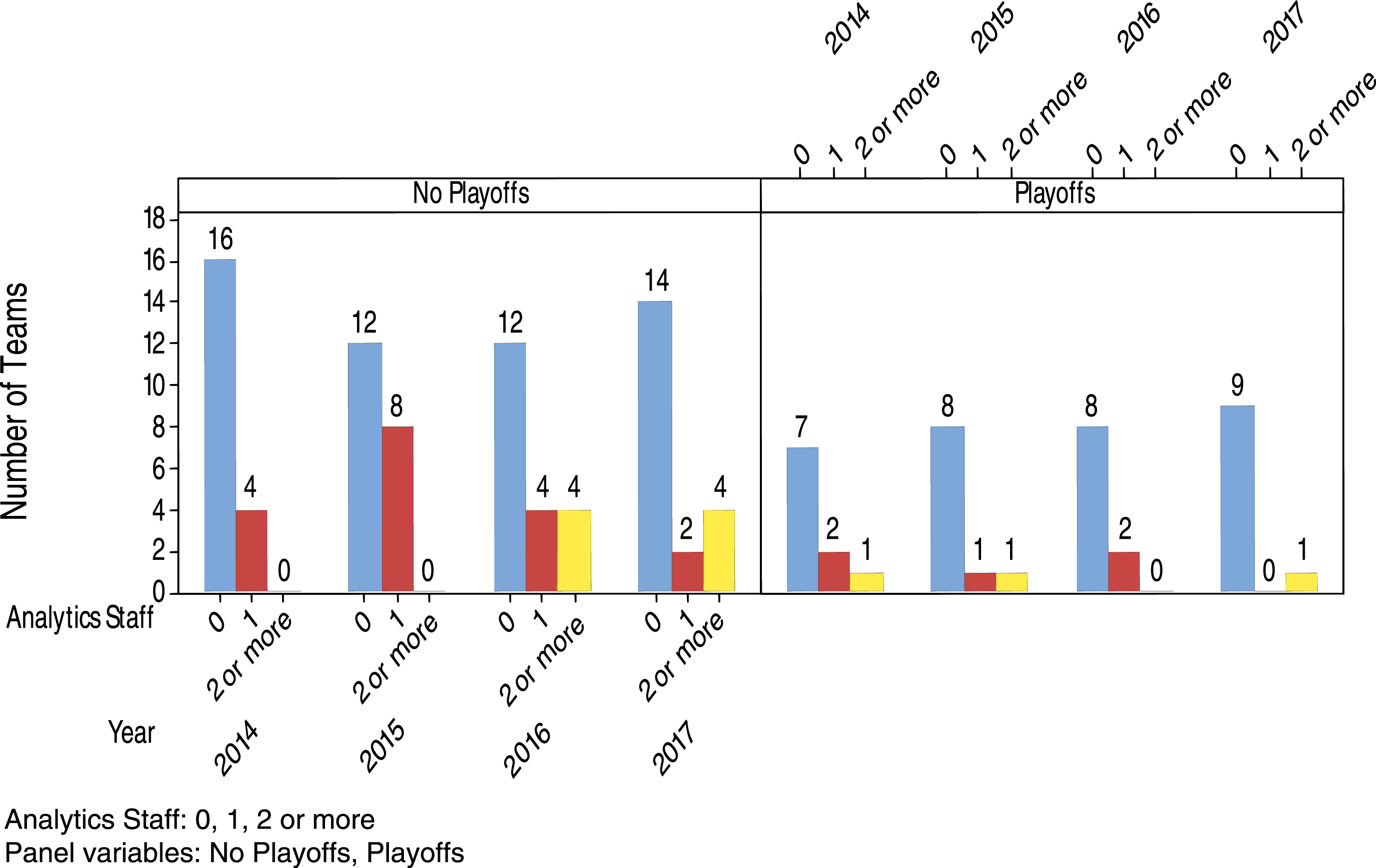
If there was no team under the condition of the conditional probability, then NA (not applicable) would be given. There were many MLB teams having no analytics department and hence no analytics staff for 2014-2017. Kansas City Royals, with four analytics staff, was a very successful team in 2014 and 2015. It advanced to the World Series but lost in 2014. Nevertheless, it became the champion of World Series in 2015. Other than Kansas City Royals, all other teams advanced to the World Series from 2014-2017 didn’t have any analytics staff. Among those last four teams of playoffs from 2014 to 2017, only Baltimore Orioles and Toronto Blue Jays each had one analytics staff. Besides the extraordinary performance of Kansas City Royals in 2014 and 2015, teams having analytics staff indicated no higher percentage of success in advancing to playoffs or during postseason in almost all conditional probabilities shown above.
3.1.3Research staff
Again from the Baseball America Directories, we compile the list of research staff (including analytics staff) employed by teams. The distribution of teams having research staff = High(7-5), Medium(4-3), Low(2-1), None(0), in no playoffs and playoffs for 2014-2017 is given in Fig. 3. The conditional probabilities below show the chances of getting into playoffs and the chances of advancing to different stages of playoffs for teams having different numbers of research staff.
P(Playoffs | Research Staff (R) = High) ≈ (0%, 50%, 20%, 50%)
P(Playoffs | R = Medium) ≈ (67%, 75%, 20%, 63%)
P(Playoffs | R = Low) ≈ (40%, 20%, 43%, 20%)
P(Playoffs | R = None) ≈ (20%, 33%, 33%, 0%)
P(Last 4 teams of playoffs | Playoffs and R = High) ≈ (NA, 0%, 0%, 67%)
P(Last 4 teams of playoffs | Playoffs and R = Medium)≈(100%, 67%, 100%, 20%)
P(Last 4 teams of playoffs | Playoffs and R = Low) ≈ (33%, 67%, 33%, 50%)
P(Last 4 teams of playoffs | Playoffs and R = None) ≈ (0%, 0%, 50%, NA)
P(Last 2 teams of playoffs | Playoffs and R = High) ≈ (NA, 0%, 0%, 0%)
P(Last 2 teams of playoffs | Playoffs and R = Medium)≈(50%, 33%, 100%, 20%)
P(Last 2 teams of playoffs | Playoffs and R = Low) ≈ (17%, 33%, 17%, 50%)
P(Last 2 teams of playoffs | Playoffs and R = None) ≈ (0%, 0%, 0%, NA)
P(Champion of World Series | Playoffs and R = High) ≈ (NA, 0%, 0%, 0%)
P(Champion of World Series | Playoffs and R = Medium) ≈ (0%, 33%, 0%, 20%)
P(Champion of World Series | Playoffs and R = Low) ≈ (17%, 0%, 17%, 0%)
P(Champion of World Series | Playoffs and R = None) ≈ (0%, 0%, 0%, NA)
Fig. 3.
Distribution of teams having research staff = High(7-5), Medium(4-3), Low(2-1), None(0), in no playoffs and playoffs for 2014-2017.
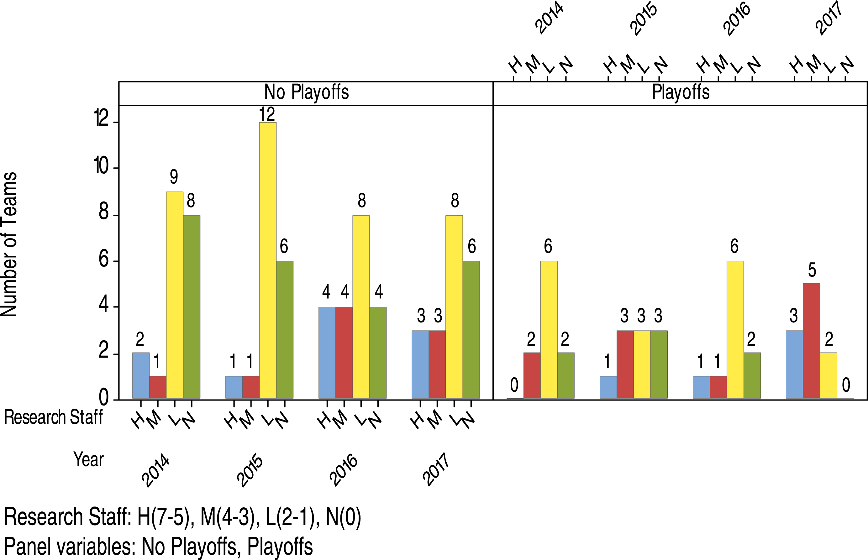
Three years out of four from 2014 to 2017, teams with research staff = Medium had higher percentages of advancing to playoffs than teams with research staff = High, Low, or None. Once teams were in playoffs, similar pattern occurred (3 years out of four) that teams with research staff = Medium had the same or higher percentages of advancing to the last 4 teams as well as the last 2 teams of playoffs than teams with research staff in other groups. Two years out of four from 2014 to 2017, teams with research staff = Medium had higher percentages of becoming the champion of World Series than teams with research staff in other groups. It appears that teams with 3 or 4 research staff (Medium group) performed most consistently than teams in other groups.
3.2Correlation coefficients
To study the correlations between different variables, we define the following notation:
W— Wins, i.e., number of games won in a regular season;
P— Team payroll;
B— Categories of analytics belief: 4(All-in), 3(Believers), 2(One-foot-in), 1(Skeptics), and 0(Non-believers);
A— Number of analytics staff;
R— Number of research staff (including analytics staff);
C— Levels of playoffs towards the championship of World Series: 5(Champion), 4(Third round game but lost), 3(Second round game but lost), 2(First round game but lost), 1(Wild card game but lost), and 0(No playoffs);
C*— C but removing 0(No playoffs).
The Pearson sample correlation coefficients for various pairs of variables for 2014-2017 are computed and displayed in Table 1. For example, r(W and P) = 0.38 (0.04) means that the Pearson sample correlation coefficient for assessing the linear relationship between W (number of games won in a regular season) and P (team payroll) is 0.38 with p-value = 0.04. Hence, the correlation between W and P is positive and significant at α = 5%. We are mostly interested in those pairs of variables whose correlations are significant (i.e., p-values < 0.05).
Table 1
Pearson sample correlation coefficients for various pairs of variables for 2014-2017, where W = wins, P = team payroll, B = categories of analytics belief, A = number of analytics staff, R = number of research staff, C = levels of playoffs towards the championship of World Series, and C*= C but removing no playoffs
| Pearson sample correlation coefficient r with p-value in parentheses | ||||
| Relationship | 2014 | 2015 | 2016 | 2017 |
| W and P | 0.38 (0.04) | 0.28 (0.13) | 0.61 (0.00) | 0.35 (0.06) |
| W and B | 0.29 (0.12) | 0.61 (0.00) | 0.44 (0.01) | 0.43 (0.02) |
| W and A | 0.20 (0.29) | –0.01 (0.94) | –0.23 (0.22) | –0.13 (0.50) |
| W and R | –0.01 (0.98) | 0.31 (0.09) | 0.06 (0.77) | 0.39 (0.03) |
| W and C | 0.67 (0.00) | 0.71 (0.00) | 0.75 (0.00) | 0.83 (0.00) |
| W and C* | –0.15 (0.69) | 0.13 (0.73) | 0.71 (0.02) | 0.68 (0.03) |
| P and B | –0.01 (0.96) | 0.14 (0.45) | 0.24 (0.20) | 0.20 (0.28) |
| P and A | –0.15 (0.43) | –0.24 (0.19) | –0.31 (0.10) | –0.02 (0.91) |
| P and R | –0.27 (0.14) | –0.27 (0.14) | –0.20 (0.29) | 0.06 (0.75) |
| P and C | 0.34 (0.07) | 0.15 (0.43) | 0.43 (0.02) | 0.45 (0.01) |
| P and C* | 0.16 (0.67) | –0.26 (0.48) | 0.06 (0.86) | 0.40 (0.25) |
| B and C | 0.12 (0.52) | 0.37 (0.04) | 0.37 (0.04) | 0.37 (0.04) |
| B and C* | –0.31 (0.39) | –0.38 (0.29) | 0.53 (0.11) | 0.61 (0.06) |
| B and A | 0.13 (0.49) | –0.05 (0.80) | –0.14 (0.45) | –0.08 (0.69) |
| B and R | 0.48 (0.01) | 0.38 (0.04) | 0.39 (0.03) | 0.35 (0.06) |
| A and C | 0.39 (0.03) | 0.34 (0.07) | –0.25 (0.18) | –0.20 (0.30) |
| A and C* | 0.42 (0.23) | 0.66 (0.04) | –0.21 (0.57) | –0.14 (0.70) |
| A and R | 0.46 (0.01) | 0.44 (0.02) | 0.33 (0.07) | 0.24 (0.21) |
| R and C | 0.16 (0.40) | 0.27 (0.16) | –0.11 (0.57) | 0.27 (0.14) |
| R and C* | 0.42 (0.23) | 0.33 (0.36) | 0.17 (0.63) | –0.10 (0.79) |
The number of games won in a regular season (W) and levels of playoffs towards the championship of World Series (C) were moderately to strongly positively correlated (r= 0.67, 0.71, 0.75, 0.83) for 2014-2017. It was because teams of fewer wins would likely not advance to playoffs and hence their value of C would be zero. Because of the zero value of C mostly coming from teams of fewer wins, the correlation between W and C tends to be positive. To see the actual effect of the number of games won in a regular season on the success in the postseason, we need to consider only those teams in the postseason, i.e., removing those teams with zero value of C. After ignoring all zeros of C (i.e., considering C*), W and levels of playoffs towards the championship of World Series in the postseason (C*) show no significant correlation at α = 5% for 2014 and 2015, but a significantly positive correlation (r= 0.71, 0.68) for 2016 and 2017. It seems that once a team is in playoffs, its standing in the regular season has a random effect on its success in the postseason. Teams of higher standings in the regular season might not generate any advantages to move forward in the postseason.
W and categories of analytics belief (B) were significantly positively correlated (r= 0.61, 0.44, 0.43) for 2015-2017.
B and C show positive correlations (r = 0.37, 0.37, 0.37) for 2015-2017. This might indicate that the categorization of analytics belief on teams could reflect the commitment made by teams that, in turn, would contribute some positive impact on the success of winning a championship of World Series. To see the actual effect of the categories of analytics belief on the success in the postseason, we consider only those teams in the postseason. B and C* show no significant correlations for 2014-2017 as all p-values are greater than 0.05. It seems that once a team is in playoffs, the analytics belief and commitment made by a team has no effect on its success in the postseason.
B and number of research staff (R) indicate a positive correlation as demonstrated by r= 0.48, 0.38, 0.39 for 2014-2016 and r= 0.35 (p-value = 0.06) in 2017.
The number of analytics staff (A) and R display some positive correlation (r= 0.46, 0.44) for 2014-2015 and r= 0.33 (p-value = 0.07) for 2016, but not for 2017.
A and C had a positive correlation (r= 0.39) in 2014, but not in 2015-2017. A and C* had a positive correlation (r= 0.66) in 2015, but not in the other three years.
R, however, does not show any significant positive or negative correlation with C or C*. R and W had a positive correlation (r= 0.39) in 2017 and r= 0.31 (p-value = 0.09) in 2015.
Table 2
Estimated values of β0, β1, β2, and β3 with their standard error in parentheses, odds ratios (eβ1, eβ2, eβ3) and their 95% CI, and p-value of the binary logistic regression model for the data of 2014-2017
| β0 | β1 | β2 | β3 | eβ1 | eβ2 | eβ3 | p-value | |
| 2014 | –1.90 | 0.51 | 0.82 | –0.32 | 1.66 | 2.27 | 0.73 | 0.31 |
| (1.04) | (0.39) | (0.65) | (0.37) | (0.77, 3.58) | (0.63, 8.09) | (0.35, 1.51) | ||
| 2015 | –4.06 | 1.22 | 0.33 | –0.13 | 3.39 | 1.38 | 0.88 | 0.03 |
| (1.59) | (0.53) | (0.57) | (0.29) | (1.19, 9.66) | (0.46, 4.19) | (0.50, 1.56) | ||
| 2016 | –2.54 | 1.15 | –0.54 | –0.55 | 3.14 | 0.58 | 0.58 | 0.03 |
| (1.42) | (0.58) | (0.80) | (0.34) | (1.01, 9.79) | (0.12, 2.77) | (0.29, 1.13) | ||
| 2017 | –1.87 | 0.11 | –0.99 | 0.45 | 1.12 | 0.37 | 1.56 | 0.09 |
| (1.06) | (0.35) | (0.74) | (0.24) | (0.56, 2.23) | (0.09, 1.58) | (0.98, 2.51) |
It is interesting to note that the team payroll (P) and W were positively correlated (r= 0.38, 0.61) in 2014 and 2016, and had r= 0.35 (p-value = 0.06) in 2017. In addition, P and C had a positive correlation (r= 0.43, 0.45) in 2016-2017 and had r= 0.34 (p-value = 0.07) in 2014. This might reflect that financial resources did have some positive impact on the journey of winning a championship of World Series. To see the actual effect of the team payroll on the success in the postseason, we need to consider C*. P and C* do not show any significant positive correlation for 2014-2017. It seems that once a team is in playoffs, its team payroll has no linear effect on its success in the postseason.
3.3Binary logistic regression models
We employ binary logistic regression models to assess the relationship between the success of advancing to playoffs and the use of sports analytics (categories of analytics belief, number of analytics staff, and number of research staff) for the data of 2014-2017. The response variable Y is the advancement to playoffs, which has the value of 1 if the team advances to playoffs and 0 if not. The continuous explanatory variable X1 is the categories of analytics belief, which has the value of 4 if the team is All-in, 3 if Believers, 2 if One-foot-in, 1 if Skeptics, and 0 if Non-believers. The variables X2 and X3 represent the number of analytics staff and number of research staff, respectively. The equation of the binary logistic regression model is
We can see from Table 2 that the p-values are both 0.03 for 2015 and 2016. Therefore there is sufficient evidence, with 5% level of significance, that the categories of analytics belief, numbers of analytics staff and research staff employed were associated with the success of a team advancing to playoffs for 2015 and 2016. However, there is insufficient evidence to indicate this association for 2014. The evidence is less convincing for 2017 as p-value = 0.09 is greater than 5% but slightly less than 10%.
Table 3
P-values of goodness-of-fit tests for binary logistic regression models for the data of 2014-2017
| Goodness-of-fit test | |||
| Pearson | Deviance | Hosmer-Lemeshow | |
| 2014 | 0.27 | 0.12 | 0.43 |
| 2015 | 0.53 | 0.30 | 0.33 |
| 2016 | 0.31 | 0.29 | 0.09 |
| 2017 | 0.31 | 0.20 | 0.90 |
The associated goodness-of-fit tests give the corresponding p-values in Table 3.
With the p-values of the goodness-of-fit tests shown in Table 3, there is insufficient evidence (with 5% level of significance) to claim that the binary logistic regression models do not fit the data adequately for 2014-2017. However, the p-value of Hosmer-Lemeshow test for 2016 is slightly less than 10%.
Table 4
Estimated values of βi, i = 0, 1, 2, . . . , 6, with their standard error in parentheses, observed F value, and p-value of the multiple linear regression model for the data of 2014-2017
| β0 | β1 | β2 | β3 | β4 | β5 | β6 | F | p-value | |
| 2014 | 75.32 | 7.43 | 12.20 | 7.67 | –0.67 | 1.30 | –0.97 | 1.38 | 0.26 |
| (6.71) | (7.90) | (7.54) | (7.64) | (7.64) | (3.07) | (1.82) | |||
| 2015 | 66.31 | 16.63 | 19.37 | 12.74 | 5.50 | –1.33 | 1.36 | 3.06 | 0.02 |
| (6.31) | (7.21) | (7.05) | (7.23) | (7.16) | (2.41) | (1.24) | |||
| 2016 | 76.83 | 8.05 | 10.46 | 5.64 | –4.45 | –1.89 | 0.02 | 1.78 | 0.15 |
| (7.71) | (8.09) | (7.98) | (8.43) | (8.23) | (2.16) | (1.43) | |||
| 2017 | 67.34 | 13.16 | 13.28 | 4.96 | 9.73 | –3.68 | 2.08 | 1.88 | 0.13 |
| (7.86) | (8.58) | (8.72) | (8.67) | (8.93) | (2.65) | (1.18) |
3.4Multiple linear regression models
We also apply multiple linear regression models to assess the relationship between the number of games won in a regular season and the use of sports analytics (categories of analytics belief, number of analytics staff, and number of research staff) for the data of 2014-2017. The response variable Y is the number of games won in a regular season. The categories of analytics belief are treated as a categorical explanatory variable, using four indicator variables X1, X2, X3 and X4 for the first four categories of analytics belief (All-in, Believers, One-foot-in, and Skeptics with Non-believers as the baseline). X5 is the number of analytics staff, and X6 is the number of research staff. The equation of the multiple linear regression model is
Minitab yielded the estimated values of parameters βi, i = 0, 1, 2, . . . , 6, with their standard error, observed F value, and p-value of the model for the data of 2014-2017. These results are presented in Table 4.
More games won in a regular season should increase the chances of moving forward to playoffs. Consequently, the number of games won in a regular season should very likely relate to the success of advancing to playoffs. By comparing 0.05 with the p-values in Table 4, we obtain the same conclusions as those in the previous section for 2014, 2015 and 2017. For 2016, the binary logistic regression model shows that, with α = 5%, the set of explanatory variables was useful for predicting the chances of advancement to playoffs. But the same set of explanatory variables was not useful for predicting the number of games won in that regular season, as shown in the multiple linear regression model. As advancing to playoffs is an important goal for teams, it seems that the binary logistic regression model is more appropriate to formulate the relationship between the success in a regular season and those explanatory variables.
Table 5
Estimated values of αi, i = 1, 2, 3, 4, and β with their standard error in parentheses, odds ratio (eβ) and its 95% CI, and p-value of the ordinal logistic regression model for the combined data of 2014-2017
| α1 | α2 | α3 | α4 | β | eβ | 95% CI | p-value | |
| X = Categories of | –0.36 | 1.49 | 2.50 | 3.31 | –0.35 | 0.70 | (0.39, 1.28) | 0.25 |
| analytics belief | (0.98) | (1.01) | (1.06) | (1.12) | (0.31) | |||
| X = Number of | –1.23 | 0.62 | 1.68 | 2.58 | –0.56 | 0.57 | (0.31, 1.06) | 0.07 |
| analytics staff | (0.40) | (0.35) | (0.45) | (0.60) | (0.32) | |||
| X = Number of | –0.99 | 0.86 | 1.85 | 2.66 | –0.20 | 0.82 | (0.58, 1.16) | 0.22 |
| research staff | (0.52) | (0.51) | (0.57) | (0.68) | (0.17) |
3.5Ordinal logistic regression models
To assess the relationship between the success of a team in the postseason and the use of sports analytics, we apply ordinal logistic regression models. Since there are only ten teams competing in playoffs each year, we have combined four years’ data together for data analysis. The response variable Y is the levels of playoffs in the postseason towards the championship of World Series, which is defined previously as C* (i.e., C without considering the value of 0). It is because those teams in playoffs have nonzero values of C. Consequently, there are five different values (5, 4, 3, 2, 1) for five different levels of playoffs towards the championship of World Series. This response variable has a natural order (i.e., champion(5) > third round(4) > second round(3) > first round(2) > wild card(1)) and can be classified as an ordinal variable. The continuous explanatory variable (or predictor) X is either (1) categories of analytics belief, (2) number of analytics staff, or (3) number of research staff. When X is the categories of analytics belief, it is defined as 4 if the team is All-in, 3 if Believers, 2 if One-foot-in, 1 if Skeptics, and 0 if Non-believers. As the response variable Y has five levels, Minitab used level 5 as the reference and formulated only four logit equations. Each equation has a unique constant, but the parameter of the predictor X is the same for all equations. The ordinal logistic regression model is
To assess the relationship between the response variable and the predictor in the ordinal logistic regression model, we test the null hypothesis that β is zero. All p-values in Table 5 are greater than 0.05. Therefore, with 5% level of significance, we conclude that no significant relationship exists between the success of a team in the postseason and any of the three analytics indicators (categories of analytics belief, number of analytics staff, and number of research staff) for the combined data of 2014-2017. Note that the evidence is less convincing when X = number of analytics staff as the p-value = 0.07.
Table 6
P-values of goodness-of-fit tests for ordinal logistic regression models for the combined data of 2014-2017
| Goodness-of-fit test | ||
| Pearson | Deviance | |
| X = Categories of analytics belief | 0.43 | 0.27 |
| X = Number of analytics staff | 0.87 | 0.73 |
| X = Number of research staff | 0.73 | 0.52 |
The associated goodness-of-fit tests give the corresponding p-values in Table 6.
Based on the p-values shown in Table 6, there is insufficient evidence, with 5% level of significance, to claim that the ordinal logistic regression models do not fit these combined four years’ data adequately.
4Effect of sports analytics after team payroll is controlled
4.1Partial correlation coefficients
4.1.1Categories of analytics belief
While the team payroll is controlled, the correlation between the success of a team and its category of analytics belief can be revealed by the partial correlation coefficient. To calculate the partial correlation coefficient (rX,Y|Z) between variables X and Y while variable Z is controlled, one may refer to the following formula given by Kutner et al. (2005).
(1)
We use formula (1) and the values of correlation coefficients listed in Table 1 to calculate the partial correlation coefficients. The partial correlation coefficients between the number of games won in a regular season (W) and the categories of analytics belief (B), while team payroll (P) is controlled, are 0.32, 0.60, 0.38, and 0.39 for 2014-2017, respectively. The positive values of the partial correlation coefficients indicate that moderately positive partial correlation existed between W and B for these four years. It suggests that the categories of analytics belief in MLB teams have some positive effect on the success of teams in the regular season, after the team payroll is taken into account.
However, the partial correlation coefficients between the levels of playoffs in the postseason towards the championship of World Series (C*) and B, while P is controlled, are -0.31, - 0.36, 0.53, and 0.59 for 2014-2017, respectively. The negative and positive values of the partial correlation coefficients indicate that random effect existed between C* and B for these four years. It suggests that the categories of analytics belief in playoffs teams have random effect on their success in the postseason, after the team payroll is taken into account.
4.1.2Number of analytics staff
Likewise, the partial correlation coefficients between W and the number of analytics staff (A), while P is controlled, are obtained as 0.28, 0.06, -0.05, and -0.13 for 2014-2017, respectively. The above positive and negative values suggest that the numbers of analytics staff employed by MLB teams have random effect on the success of teams in the regular season, after the team payroll is taken into account.
In addition, the partial correlation coefficients between C* and A, while P is controlled, are 0.45, 0.64, - 0.20, and -0.14 for 2014-2017, respectively. Again, the positive and negative values suggest that the numbers of analytics staff employed by playoffs teams have random effect on their success in the postseason, after the team payroll is taken into account.
4.1.3Number of research staff
The partial correlation coefficients between W and the number of research staff (R), while P is controlled, are 0.10, 0.42, 0.23, and 0.39 for 2014-2017, respectively. The above positive values suggest that the numbers of research staff hired by MLB teams have some positive effect on the success of teams in the regular season, while the team payroll is controlled.
However, the partial correlation coefficients between C* and R, while P is controlled, are 0.49, 0.28, 0.19, and -0.14 for 2014-2017, respectively. The positive and negative values suggest that the numbers of research staff hired by playoffs teams have random effect (perhaps slightly positive effect) on their success in the postseason, while the team payroll is controlled.
4.2Partial F tests
When the team payroll is used in the regression model as an explanatory variable to predict the number of games won in a regular season, does the addition of the information of (1) categories of analytics belief, (2) number of analytics staff, or (3) number of research staff significantly improve the predictability of the regression model?
4.2.1Categories of analytics belief
To investigate the above question, we first consider the reduced model consisting of the team payroll (logarithmic value) X1 as the only continuous explanatory variable. Then we consider the full model consisting of team payroll (logarithmic value) X1 and the categories of analytics belief as a categorical explanatory variable using four indicator variables X2, X3, X4, and X5. The response variable Y is the number of games won in a regular season. The model equations are:
To test the null hypothesis that
The test statistic is
Table 7
Estimated values of β0, β1,
| (1) Categories of analytics belief | |||||||||||||
| β0 | β1 |
|
|
|
|
|
| SSEr | SSEf | F | p | ||
| 2014 | –94 | 9.46 | –73 | 8.07 | 4.97 | 10.4 | 4.67 | –2.31 | 2302 | 1746 | 1.91 | 0.14 | |
| (83) | (4.5) | (81) | (4.4) | (6.7) | (7.0) | (7.1) | (7.0) | ||||||
| 2015 | –80 | 8.62 | –25 | 4.99 | 18.2 | 17.7 | 10.7 | 4.76 | 2901 | 1779 | 3.79 | 0.02 | |
| (100) | (5.4) | (91) | (4.9) | (6.8) | (7.2) | (7.2) | (7.1) | ||||||
| 2016 | –303 | 20.5 | –267 | 18.6 | 3.25 | 1.01 | –0.17 | –8.78 | 2002 | 1458 | 2.24 | 0.10 | |
| (90) | (4.8) | (90) | (4.9) | (6.3) | (6.8) | (6.7) | (6.5) | ||||||
| 2017 | –145 | 12.0 | –139 | 11.3 | 14.5 | 6.3 | 2.0 | 5.2 | 3450 | 26.76 | 1.74 | 0.17 | |
| (125) | (6.6) | (124) | (6.7) | (8.3) | (8.8) | (8.7) | (8.7) | ||||||
| (2) Number of analytics staff | |||||||||||||
|
|
|
| SSEr | SSEf | F | p | |||||||
| 2014 | –112 (81.8) | 10.35 (4.41) | 3.08 (2.07) | 2302 | 2129 | 2.21 | 0.15 | ||||||
| 2015 | –87 (105) | 9.01 (5.60) | 0.72 (2.42) | 2901 | 2891 | 0.09 | 0.77 | ||||||
| 2016 | –296 (96.9) | 20.13 (5.15) | –0.38 (1.67) | 2002 | 1998 | 0.05 | 0.82 | ||||||
| 2017 | –144 (0.26) | 12.03 (6.69) | –1.73 (2.42) | 3450 | 3386 | 0.51 | 0.48 | ||||||
| (3) Number of research staff | |||||||||||||
|
|
|
| SSEr | SSEf | F | p | |||||||
| 2014 | –113 (88.3) | 10.41 (4.74) | 0.81 (1.24) | 2302 | 2267 | 0.42 | 0.52 | ||||||
| 2015 | –149 (94.7) | 12.1 (5.06) | 2.84 (1.09) | 2901 | 2321 | 6.75 | 0.02 | ||||||
| 2016 | –330 (91.4) | 21.8 (4.85) | 1.14 (0.89) | 2002 | 1885 | 1.67 | 0.21 | ||||||
| 2017 | –131 (117) | 10.99 (6.24) | 2.07 (0.95) | 3450 | 2676 | 1.74 | 0.17 | ||||||
4.2.2Number of analytics staff
The reduced model remains unchanged. The full model becomes
4.2.3Number of research staff
The reduced model remains unchanged. The variable X2 in the full model shown in Section 4.2.2 is changed to the number of research staff. Nonetheless, the corresponding null hypothesis, the numerator and denominator degrees of freedom of F remain intact. Inspecting the p-values in the third part of Table 7, we conclude (with α = 5%) that once the team payroll was already in the model, the addition of the information of the number of research staff was not statistically significantly useful in the regression model for predicting the number of games won in a regular season for 2014, 2016 and 2017. However, we obtain the conclusion of statistical significance for 2015.
4.3Model utility F test
To test if both the team payroll and the use of sports analytics are good predictors of the success in playoffs towards the championship of World Series, we apply the model utility F test to the combined postseasonal data of 2014-2017. Thus there are altogether forty data points for analysis, instead of ten data points in each year. The response variable Y is the levels of playoffs in the postseason towards the championship of World Series: 5(Champion), 4(Third round game but lost), 3(Second round game but lost), 2(First round game but lost), 1(Wild card game but lost). For simplicity, we assume that Y is a continuous variable. The four continuous explanatory variables are the team payroll (logarithmic value) X1, categories of analytics belief X2, number of analytics staff X3, and number of research staff X4. The variable X2 has the values: 4(All-in), 3(Believers), 2(One-foot-in), 1(Skeptics), and 0(Non-believers); it is assumed to be a continuous variable. The equation of the multiple linear regression model is
Minitab calculated the estimated values of the regression parameters βi’s with their standard error, observed F value, and p-value of the model for the combined data of 2014-2017. The results are given in Table 8.
Fig. 4.
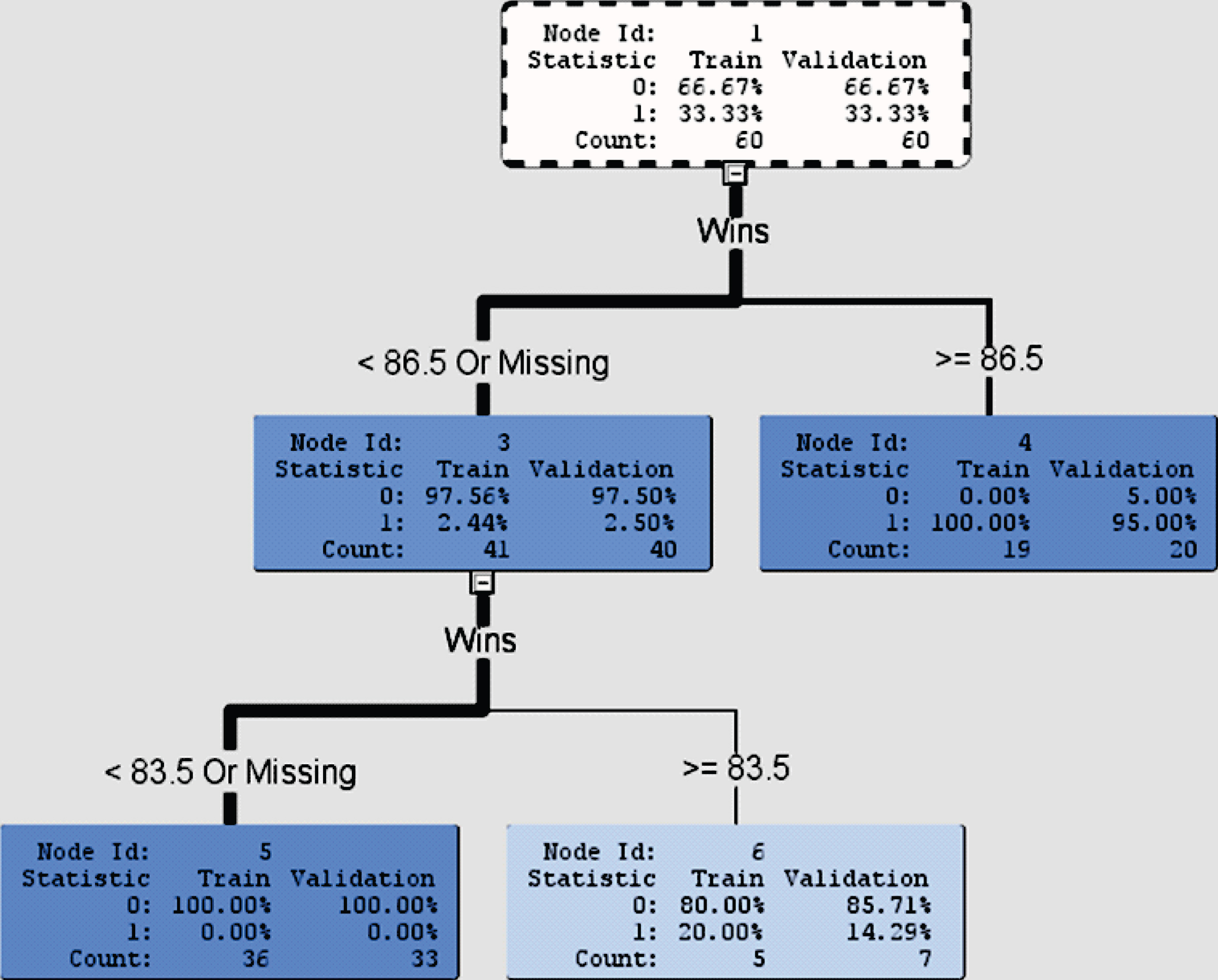
Decision tree for binary target variable with Wins as an input variable.
The model utility F test is to test the null hypothesis that β1 = β2 = β3 = β4 = 0 . As the p-value is 0.12, we conclude (with 5% level of significance) that the team payroll, categories of analytics belief, number of analytics staff, and number of research staff are not good predictors in the multiple linear regression model for the success in playoffs. This conclusion agrees with Schwartz and Zarrow (2009) that the success in October (i.e., playoffs) can be viewed as a truly random event.
Table 8
Estimated values of βi’s with their standard error in parentheses, observed F value, and p-value of the multiple linear regression model for the combined data of 2014-2017
| β0 | β1 | β2 | β3 | β4 | F | p-value |
| –16.9 | 0.97 | 0.26 | 0.49 | 0.07 | 1.99 | 0.12 |
| (12) | (0.63) | (0.20) | (0.22) | (0.12) |
5Decision trees
The predictive modeling of decision trees will be used to classify MLB teams for their success in the regular season and postseason. There are 30 teams in MLB, and only 10 teams move on to playoffs each year. The data collected in one year, however, are not adequate to come up with meaningful predictive models. Rather, we will combine four years’ data (2014-2017) to have 120 teams (or instances) to build the predictive models.
5.1Wins as an input variable available
5.1.1Binary target variable
The target (or response) variable is the advancement to playoffs, which has the value of 1 if the team advances to playoffs and 0 if not. The input variables are catchers’ salary, infielders’ salary, outfielders’ salary, pitchers’ salary, team payroll, and Wins (number of games won in a regular season). In addition, the input variables include the number of analytics staff, the number of research staff as well as four indicator variables for the categories of analytics belief: All-in, Believers, One-foot-in, and Skeptics with Non-believers as the baseline. SAS Enterprise Miner workstation 14.2 with interactive mode was used to implement the algorithms to build the predictive model. The decision tree is given in Fig. 4.
Node 1 shows that the data are randomly selected into the training model (60 teams) and the validation model (60 teams). Among the 60 teams in both the training and validation models, 66.67% of them were not in playoffs whereas 33.33% of them were.
The decision tree shows that Wins is the variable first chosen among all input variables mentioned above to split the tree. Since there are no missing observations in our data set, the corresponding test condition is < 86.5 or ≥ 86.5 games. This means that the decision tree classifies teams in each of the training and validation models into 2 groups, one group in Node 3 with teams winning less than 86.5 games (i.e., less than or equal to 86 games) in a regular season and the other group in Node 4 with teams winning at least 86.5 games (i.e., greater than or equal to 87 games) in a regular season. The 60 teams in the training model are separated into 41 teams in Node 3 and 19 teams in Node 4. Likewise, the 60 teams in the validation model are separated into 40 teams in Node 3 and 20 teams in Node 4. In Node 3, 2.44% of the 41 teams in the training model and 2.50% of the 40 teams in the validation model advanced to playoffs. In Node 4, however, all 19 teams (100%) in the training model and 95% of the 20 teams in the validation model advanced to playoffs. SAS then chose the input variable Wins again to split Node 3 with the new test condition: < 83.5 or ≥ 83.5 games. For those teams winning less than 83.5 games in a regular season in Node 5, none of the 36 teams in the training model and none of the 33 teams in the validation model advanced to playoffs. For those teams winning at least 83.5 games (but less than 86.5 games), there was only 1 team out of 5 teams (20%) in the training model and also only 1 team out of 7 teams (14.29%) in the validation model advanced to playoffs.
Therefore, from the decision tree in Fig. 4, we may conclude that teams winning 87 games or more is very highly likely to advance to playoffs, teams winning between 84 and 86 games (inclusive) still have a small chance of moving on to playoffs, and teams winning 83 games or fewer in a regular season have no chance of advancing to playoffs. As 162 games are played by each team in a regular season, 87 wins translate to 0.537 winning percentage and 83 wins to 0.512 winning percentage.
The misclassification rates for the training model and validation model are 1.67% and 3.33%, respectively. In addition, the average squared errors are 0.0133 and 0.0313 for the training model and validation model, respectively. As a result, we conclude that the test conditions (< 83.5 games and ≥ 86.5 games) of the input variable Wins are excellent criteria to classify MLB teams into no playoffs or playoffs.
5.1.2Ordinal target variable
With all the input variables given in Section 5.1.1, the target variable is considered to be the levels of playoffs towards the championship of World Series. The target variable has 6 levels: 0(No playoffs), 1(Wild card game but lost), 2(First round game but lost), 3(Second round game but lost), 4(Third round game but lost), and 5(Champion). It will be treated as an ordinal variable. The outcome of a decision tree is displayed in Fig. 5.
In Node 1, all 120 teams are randomly divided approximately 50-50 into the training and validation models according to their stages towards the championship of World Series. In fact, 59 teams and 61 teams go to the training and validation models, respectively. The input variable Wins with the same test condition (< 86.5 or ≥ 86.5 games) is first chosen among all the given input variables to split the decision tree. Among the 59 teams in the training model, 40 teams go to Node 3 as their wins are less than 86.5 games and 19 teams go to Node 4 as their wins are 86.5 games or more. Likewise, among the 61 teams in the validation model, 41 teams go to Node 3 and 20 teams go to Node 4. Wins less than 86.5 games in a regular season is an excellent predictor to classify 100% of the teams in training model and 95.12% of the teams in validation model as target 0 (i.e., no playoffs). There is only one team (2.44%) in the validation model having target 1 (i.e., wildcard game but lost), and also only one team having target 2 (i.e., first round game but lost).
Node 4 shows that none of the 19 teams in the training model and only 1 team out of 20 teams (5%) in the validation model has target 0(no playoffs). It means that 38 of 39 teams (97.4%) with 86.5 wins or more in a regular season go to playoffs. As four teams out of the ten playoffs teams go to the first round game but lost, target 2 in Node 4 has the highest percentage for both models, 42.11% of teams in the training model and 35% of teams in the validation model. Apart from this observation, however, both training and validation models do not display any distinct patterns on different stages towards the championship of World Series.
Fig. 5.
Decision tree for ordinal target variable with Wins as an input variable.
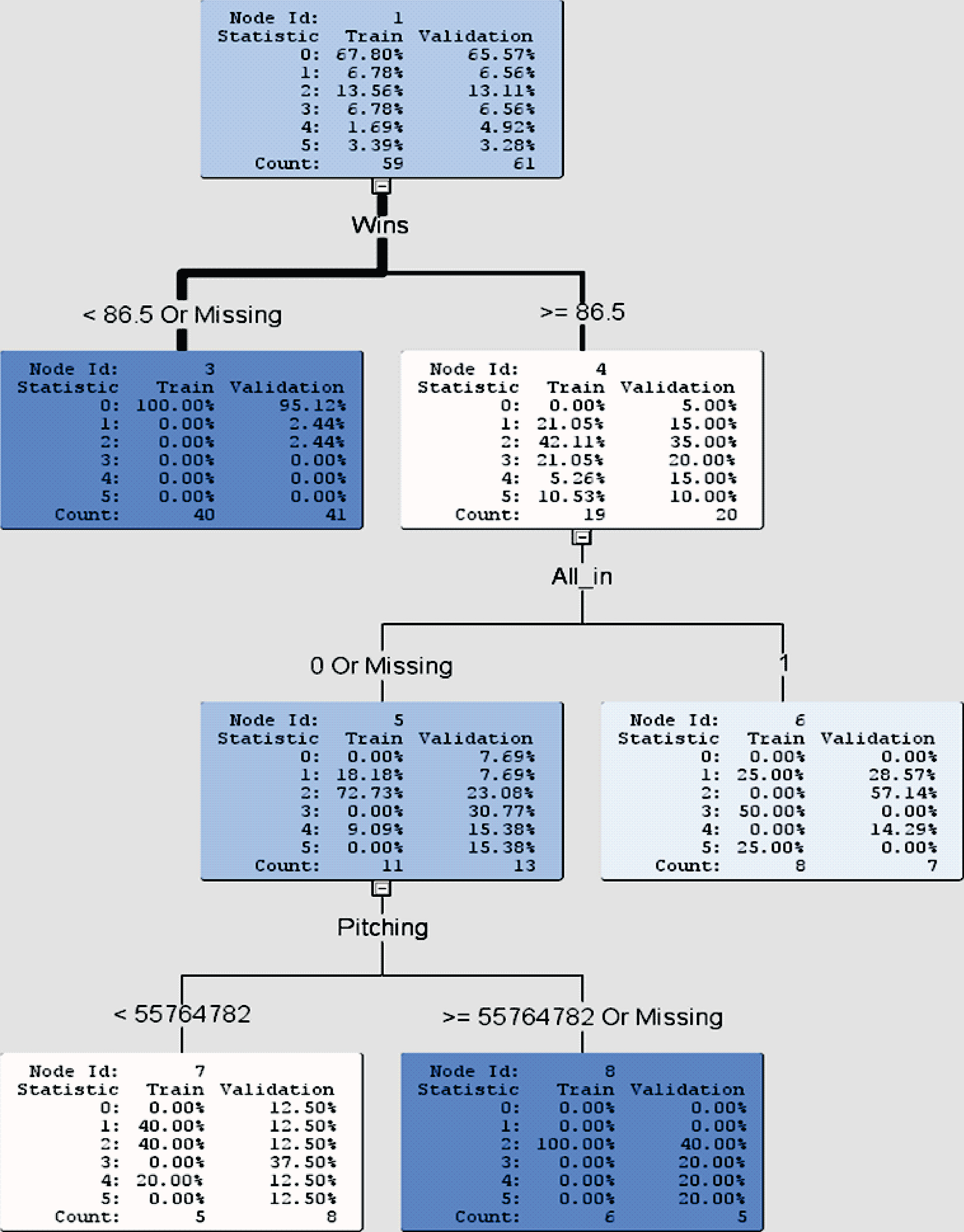
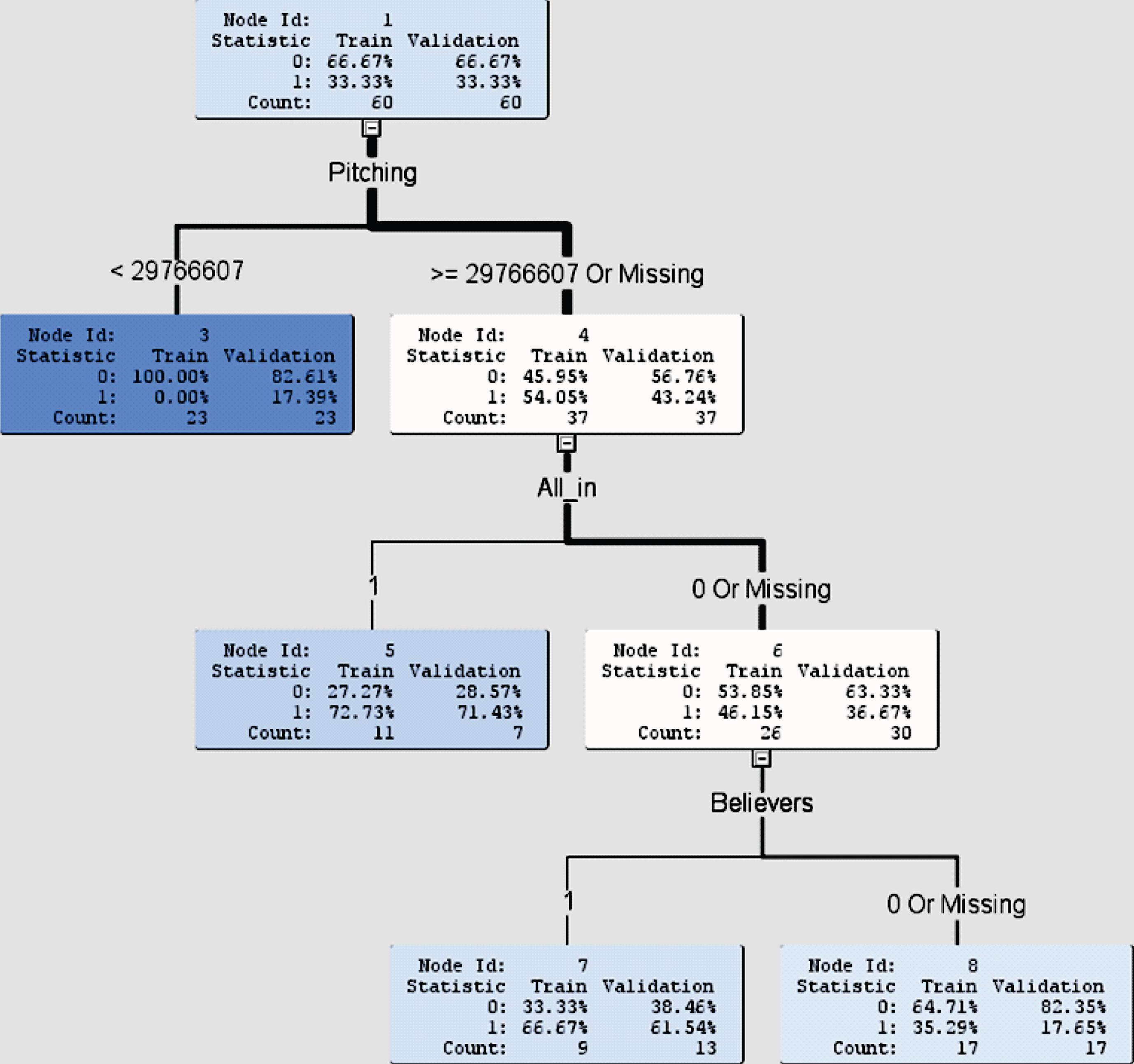
Fig. 6.
Decision tree for binary target variable without Wins as an input variable.
The input variable All_in is then chosen to further split Node 4. In Node 5 (when teams are not All_in), it looks like more teams have lower target values (1 and 2) in the training model and teams spread evenly with slightly higher target values in the validation model. In Node 6 (when teams are All_in), however, it seems that teams spread more widely across the targets with three spikes at targets 1, 3, 5 in the training model, and teams have lower targets (1 and 2) in the validation model.
Afterwards, the input variable pitchers’ salary with the test condition (< 55,764,782 or ≥ 55,764,782) is used to split Node 5 further. For not All_in teams winning at least 87 games in a regular season and pitchers’ salary at least $55.7 million (approximately), Node 8 shows that they have higher targets (2-5) in the validation model and concentrate on target 2 in the training model. Node 7, however, shows that these not All_in teams with pitchers’ salary less than $55.7 million (approximately) spread more evenly across the targets in both the validation and training models.
The misclassification rates for the training and validation models are 11.86% and 31.15%, respectively. The average squared errors for the training and validation models are 0.0232 and 0.0752, respectively. This decision tree yields moderately accurate predictions for classifying MLB teams into different stages of playoffs towards the championship of World Series.
5.2Wins as an input variable not available
At the beginning of a MLB season in late March, the information of the number of games won in a regular season is certainly not available. In this situation, one may still wish to build a decision tree to classify teams into no playoffs (target 0) or playoffs (target 1). As the target variable is binary, we can use the same procedure as shown in Section 5.1.1 but without Wins as an input variable. The decision tree is presented in Fig. 6.
Node 1 shows that the data are randomly selected into the training model (60 teams) and validation model (60 teams). The first input variable chosen is pitchers’ salary with the test condition (< 29,766,607 or ≥ 29,766,607). Under this test condition, the 60 teams in each of the training and validation models are separated into 23 teams in Node 3 and 37 teams in Node 4 in their respective model. In Node 3 (pitchers’ salary < ≈ $29.7 million), none of the 23 teams in the training model and 17.39% of the 23 teams in the validation model advanced to playoffs. In Node 4 (pitchers’ salary ≥ ≈ $29.7 million), however, 54.05% of the 37 teams in the training model and 43.24% of the 37 teams in the validation model advanced to playoffs. Consequently, pitchers’ salary with a threshold of approximately $29.7 million played an important role to identify whether or not the team had a higher chance of moving on to playoffs.
Under Node 4, further classification takes place. The second input variable chosen is All_in with the test condition: 1(yes) or 0(no). Under this test condition, the 37 teams in the training model are separated into 11 teams in Node 5 and 26 teams in Node 6. Likewise, the 37 teams in the validation model are separated into 7 teams in Node 5 and 30 teams in Node 6. For teams that were All_in, Node 5 shows that 72.73% of the 11 teams in the training model and 71.43% of the 7 teams in the validation model advanced to playoffs. However, Node 6 shows that 46.15% of the 26 teams in the training model and 36.67% of the 30 teams in the validation model advanced to playoffs. In addition to spending at least $29.7 million on pitchers’ salary, the All_in teams would significantly increase their chances of advancing to playoffs. For teams that were not All_in but were Believers instead, Node 7 indicates that their chances of advancing to playoffs were 66.67% and 61.54% in the training and validation models, respectively. These percentages were much higher than those (35.29% and 17.65%) in Node 8 for teams that were not Believers either.
The misclassification rates for the training model and the validation model are 20% and 23.33%, respectively. The average squared errors produce 0.1344 and 0.1923 for the training and validation models, respectively. This decision tree yields moderately accurate predictions for classifying MLB teams into no playoffs or playoffs.
6Summary and concluding comments
The relationship between the use of sports analytics and the success in regular season and postseason in MLB has been studied through the empirical data of 2014-2017. The use of sports analytics can be examined by (1) the categories of analytics belief given by ESPN in The Great Analytics Rankings, (2) the number of analytics staff worked in the analytics department, and (3) the total number of research staff (including analytics staff) employed by a team. Several good indicators are identified to be useful for predicting the success in the regular season. They are Wins (number of games won in a regular season), categories of analytics belief, and team payroll (in particular, the pitchers’ salary).
Fig. 4 illustrates that for a MLB team winning 87 games or more in a regular season, the chance of the team advancing to playoffs is at least 95%. On the contrary, for a MLB team winning 83 games or fewer in a regular season, it has no chance of getting into playoffs. Teams that win between 84 and 86 games (inclusive) in a regular season have about 14-20% chances of moving on to playoffs. Winning 87 games out of 162 games in a regular season translates to the winning percentage of 0.537. This winning percentage can be regarded as an important goal that teams would like to achieve in a regular season.
From Fig. 1, we can see that on average 77.5% of the playoffs teams came from the category of BELIEVERS (All-in, Believers) and only 22.5% came from the category of NON-BELIEVERS (One-foot-in, Skeptics, Non-believers). Moreover, we obtain the results that about 48% of the BELIEVERS’ teams and about 16% of the NON-BELIEVERS’ teams moved on to playoffs during 2014-2017. These outcomes may encourage MLB teams which are currently in the level of One-foot-in, Skeptics or Non-believers to re-consider their engagement with the sports analytics.
From Fig. 2, we obtain the results that about 37%, 22%, and 27% of teams with the number of analytics staff = 0, 1, and 2 or more, respectively, advanced to playoffs during 2014-2017. In addition, we obtain from Fig. 3 that about 33%, 55%, 31%, and 23% of teams with the number of research staff = High(7-5), Medium(4-3), Low(2-1), and None(0), respectively, advanced to playoffs during these four years. These results might suggest that analytics staff alone may not be able to show the positive effect on the teams. Therefore, other research staff such as the ones working in the areas of mathematical modeling, data science, informatics, research and development, etc. should also be employed to complement the work of analytics staff.
Total team payroll has long been identified as an essential component for the success of a team in the regular season. From the decision tree in Fig. 6, we can see that teams with pitchers’ salary at least $29.7 million would have about 72% and 64% chances of advancing to playoffs if their categories of analytics belief are All_in and Believers, respectively. This area with the payroll amount might provide management teams with some guidelines on where and how much they need to allocate their financial resources to players for a successful regular season.
So far there haven’t been any good predictors found for the success in the postseason. It seems that once teams have advanced to the postseason, the playoffs teams start with a clean slate. Perhaps the factors of the excitement of playoffs, more media coverage, and high expectations from baseball fans might transform the playoffs teams to different levels of intensity and eagerness to compete. However, it is very difficult to quantify these factors.
The limitation of this study is that it involves only four years’ empirical data. Teams that are rebuilding might not maximize wins in a season or two. The improvement of teams’ performance and optimizing the wins might take place in the medium to long term. Consequently, more data are necessary for further study of the long-term effect of the sports analytics on the success of teams in regular season and postseason. In order to control for teams that are rebuilding in a season or are competing for the playoffs, one might consider the preseason projected wins from some projection systems such as PECOTA, Steamer, and ZiPS. If a team’s belief in analytics has a positive impact on the team, then it should outperform its projected wins. This notion is worth pursuing in the future. The changes of MLB teams’ categories of analytics belief, such as changing from One-foot-in to Believers, should be made known and updated in The Great Analytics Rankings. This updated information would be crucial for future data analysis.
Acknowledgments
The authors are grateful to a referee for many valuable suggestions.
References
1 | Baseball-reference.com, 2014-2017. ‘MLB Standings ’. URL: https://www.baseball-reference.com/leagues/MLB/2014-standings.shtml (Substitute 2015, 2016, and 2017 for 2014 to get the corresponding URL.) |
2 | Espn.com, 2015. ‘The Great Analytics Rankings’. URL: https://www.espn.com/espn/feature/story/_/id/12331388/the-great-analytics-rankings |
3 | Kutner, M ., Nachtsheim, C ., Neter, J ., Li, W. , (2005) . Applied Linear Statistical Models. 5th ed. McGrawHill, pp. 271. |
4 | Sbnation.com, 2014, 2015, 2016, 2017. ‘MLB Playoffs’. URLs: https://www.sbnation.com/mlb/2014/9/29/6859873/2014-mlb-Playoffs-schedule-bracket-format https://www.sbnation.com/mlb/2015/10/6/9460931/2015-mlb-Playoffs-schedule-postseason-bracket-results-teams https://www.sbnation.com/mlb/2016/10/4/13100224/2016-mlb-Playoffs-schedule-postseason-bracket-results-teams https://www.sbnation.com/mlb/2017/10/3/16390256/2017-mlb-Playoffs-bracket-schedule-scores-results-postseason |
5 | Schwartz, N ., Zarrow, J. , (2009) . An analysis of the impact of team payroll on regular season and postseason success in Major League Baseball, Undergraduate Economic Review 5: (1), Article 3. URL: http://digitalcommons.iwu.edu/uer/vol5/iss1/3 |
6 | Spotrac.com, 2014-2017. ‘MLB Team Payroll’. URL: https://www.spotrac.com/mlb/payroll/2014/ (Substitute 2015, 2016, and 2017 for 2014 to get the corresponding URL.) |


