
Football under pressure: Assessing malfeasance in Deflategate
Abstract
After the 2015 AFC Championship game between the New England Patriots and the Indianapolis Colts, the Patriots were accused of deflating their footballs to gain an unfair advantage over their opponents. A subsequent investigation by the NFL led to the publication of a report named after Ted Wells, its main author. The Wells report’s central conclusion was that the Patriots and their quarterback, Tom Brady, were at least generally aware of what was deemed to be probable illicit behavior by some of the Patriots employees responsible for football preparation. NFL commissioner Roger Goodell then penalized team and player with fines, draft pick losses, and suspensions. This article evaluates the statistical analysis in the Wells report and finds fault with the set of hypotheses it tests, the way in which it tests them, the robustness of its test results, and the conclusions it draws from its tests. We also highlight problems with the quality of the data used in the report, and sketch a more appropriate interpretation of the evidence presented to the NFL. We conclude by discussing the use and interpretation of statistical evidence in legal and quasi-legal procedures generally.
1Introduction
The American Football Conference (AFC) Championship game for the 2014-2015 National Football League (NFL) season, between the New England Patriots and the Indianapolis Colts, took place on January 18th, 2015.1 It ended in a 45-7 victory for the Patriots. During and especially after the game, the Patriots were accused of deflating their footballs in order to gain an unfair advantage. A subsequent investigation by the NFL led to the publication on May 6th of a report hereafter referred to as the Wells report, after lawyer Ted Wells, its lead author (Wells, Karp, and Reisner 2015). The Wells report’s central conclusion is that the Patriots’ quarterback, Tom Brady, was at least “generally aware” of what was deemed to be “more probable than not” illicit behavior by some of the Patriots employees responsible for football preparation. The next week, team and player were penalized with fines, draft pick losses, and suspensions by NFL commissioner Roger Goodell. The National Football League Players Association (NFLPA), on behalf of Brady, proceeded to appeal his suspension. A 10-hour hearing ensued on June 23rd (National Football League, 2015), and on July 28th Goodell decided to uphold his initial judgment. In response, the NFL filed suit in federal court in an attempt to persuade a federal judge to uphold this decision. On September 3, Judge Berman of the United States District Court for the Southern District of New York vacated the suspension. The NFL announced almost immediately that it would appeal, but Brady will be able to compete from the start of the 2015-2016 NFL season.
This article evaluates a key element in the controversy, better known as Deflategate: the statistical analysis in the Wells report. This analysis was used in the report to demonstrate or at least suggest that there was convincing evidence that the balls used by the Patriots during the AFC Championship Game were indeed deflated, i.e., measured pressure levels at half time were lower than natural factors could explain. In what follows, we focus on a number of aspects of this analysis. After providing some more background on Deflategate and the Wells report, we first discuss the data the statistical analysis in the Wells report relies upon, and how they were collected. We then present and evaluate the set of hypotheses that were tested, the way in which they were tested, the robustness of the test results, and the conclusions drawn from its tests. Based on this evaluation, we sketch what we believe to be an appropriate interpretation of the evidence presented in the Wells report. We conclude by discussing the use of statistical evidence in disciplinary procedures more broadly, the legal standard to which such evidence is typically held in court, and whether the statistical analysis in the Wells report appears to meet that standard.
2Deflategate and the Wells Report
The central questions in the Deflategate affair were whether the New England Patriots impermissibly deflated the footballs they played with during the 2015 AFC Championship game, and, if so, whether their quarterback, Tom Brady, knew about this or even arranged for the footballs to be deflated. These are the questions the Wells report attempted to answer based on the “preponderance of the evidence,” not the higher standard of “beyond a reasonable doubt.” It does so by drawing on various different types of evidence: interviews with actors involved, including NFL employees, game officials, and Patriots personnel; data on air pressure, weather, temperature, footballs, and gauges; as well as a broad variety of documents such as emails, league rules, text messages, and security footage. It also incorporates certain results from consultation with outside experts, in particular findings from experiments, tests, and analyses carried out by Exponent, a scientific and engineering consulting firm.
These inputs, combined with various edits by NFL in-house lawyer Jeff Pash (Berman, 2015), led to a 243-page report: 139 pages (plus front matter) of main text (“Main Text”), plus two appendices prepared by Exponent, the first of which (“Appendix 1”) includes 68 pages (plus front matter) and is itself followed by an appendix (“Statistical Analysis Appendix”), while the second one (“Appendix 2” is a four-page letter. Together these components provide the following main sets of findings: a discussion of the investigation process; a timeline of events as they occurred during and around the AFC Championship Game; an analysis of communications between Tom Brady and Patriots equipment staff before and after the game; an overview of certain experimental findings that touch upon various aspects of the science of football inflation; and a statistical analysis of the level of air pressure in the Patriots footballs used during the game.
This last set of findings, the statistical analysis, is presented in Section VIII of the main text, in the “Analysis of Data Collected at Halftime” section of Appendix 1, and in the Statistical Analysis Appendix. The analysis, which was carried out by Exponent, addresses a more focused question than the Wells report as a whole: were the footballs that the Patriots used during the first half of the game less inflated than one would expect if no improprieties had taken place?2 If they were not, the other elements of the report –which we take as given here - may well seem superfluous. The Wells report’s answer to this question is the subject of our evaluation in this article. We discuss the statistical analysis in Section IV below, and evaluate it in Section V. Before turning to those, we introduce the data analyzed in that analysis, and how they were collected and reported, so as to assess their reliability and usefulness.
3Data
The data set on which the statistical analysis in the Wells report is based is surprisingly small: it consists of 30 observations. These observations are the pressure readings taken by two different officials during halftime of 15 different footballs: 11 Patriots footballs, and four Colts footballs. Figure 1, which displays Table 1 in Appendix 1 in the Wells report, shows these values organized by team, ball, and official.
It is not known exactly when these measurements were taken. This is important because after the footballs were brought inside at halftime, they warmed up, which gradually increased the measured air pressure. The Wells report concludes that there are two possible scenarios (Wells et al., 2015):
– The Patriots footballs were measured first, followed by the Colts footballs, after which those Patriots footballs that were deemed not sufficiently inflated were re-inflated;
– The Patriots footballs were measured first, followed by reflation of those Patriots footballs that were deemed not sufficiently inflated, and only then were the Colts footballs measured.
Beyond this basic question of the order in which these three sets of actions took place, there is also no record of the duration of each actions or the time that passed in between actions or sets of actions. What is known is the reason why only four Colts footballs were measured: the officials ran out of time, which suggests to us that the second scenario is the more likely one.
It is also not known with certainty which gauge was used for each particular measurement. There are (at least) two gauges that were used to measure air pressure at halftime: one has a red Wilson logo on it (the “Logo Gauge,” as it is referred to in the Wells report), and one that does not (the “Non-Logo Gauge”). This is important, because the different gauges do not produce the same readings: according to Exponent, the Logo Gauge produces readings that are 0.3-0.4 psi higher than the readings produced by the Non-Logo Gauge (Wells et al., 2015). The Wells report considers four different versions of the data collected to account for uncertainty as to which gauge was used for each of the 30 measurements:
1) Official Blakeman (“Official 1”) used the Non-Logo Gauge for all 15 of his measurements, while official Prioleau (“Official 2”) used the Logo Gauge for all 15 of his measurements;
2) As in 1), but assuming that the officials switched gauges after measuring the 11 Patriots footballs;
3) As in 2), but assuming that the measurements produced by the two officials for the third Colts football were written down in the wrong column;
4) As in 2), but without taking the measurements of the third Colts football into account.
The adjustment applied to the raw data in version 2) makes it so that for each of the two teams, the official using the Logo Gauge is associated with air pressure measurements that are on average higher, while the adjustment applied to the raw data in version 3) makes it so the that for each individual football the official using the Logo Gauge is associated with a higher measured air pressure value. This version 3) of the dataset is Exponent’s preferred version. The gauge swap between teams appears to lend support, again, to the idea that the most likely scenario for the order of the three sets of actions is the second one. The intervening reflation of the Patriots footballs would have produced a longer window of opportunity, with more different actions contained in it, than the direct the succession of measurement session of the first scenario.
Even undisputable levels of air pressure observed at precise moments during halftime, low as they may be, would not, of course, suffice to determine whether the air pressure levels in the Patriots footballs were illicitly lowered before the start of the game. The statistical analysis in the Wells report relies on a number of additional assumptions and findings regarding the state of the footballs both before and after the Championship Game in its efforts to determine whether that was the case.
First, it relies on referee Walt Anderson’s recollection, supported by both teams’ preferred air pressure levels, that the air pressure of the footballs before the game (before any potential malfeasance took place) was near 12.5 psi for the Patriots footballs and 13.0 or 13.1 psi for the Colts footballs. There is no record of this.
Second, it assumes that Anderson made these measurements using the Non-Logo Gauge. This assumption is the opposite of Anderson’s recollection, and the report recognizes that “uncertainty” remains surrounding the question of which gauge was used before the game. After the report’s release, Ted Wells stated that this question was irrelevant: “it doesn’t matter because regardless of which gauges were used the scientific consultants addressed all of the permutations in their analysis” (Boston Globe, 2015). We will show in Section V that this statement is incorrect.
Third, the report discards air pressure measurements taken after the game as unreliable. Four footballs were randomly selected after the game, and their air pressure levels were measured and recorded by the same officials who produced the halftime measurements. According to the Wells report, “the pressure levels at which these eight footballs started the second half (..) is [sic] significantly less certain than the information (..) concerning the pre-game or halftime periods.”
Fourth, the report largely ignores a 12th Patriots football’s air pressure. This football was intercepted by Colts player D’Qwell Jackson during the first half. Colts equipment personnel suspected that this football was underinflated, and alerted NFL officials, who took three measurements of the football’s pressure level. The report discusses these measurements, but does not derive conclusions from them.
We now discuss how the Wells report did and did not use the data and assumptions discussed in this section to reach its conclusions.
4Statistical model and results in the wells report
The Wells report essentially uses a difference-in-differences estimator to determine whether the Patriots footballs were potentially deflated illicitly between the time when Walt Anderson measured their air pressure levels and when they were measured at halftime. This estimator tests whether the drop in pressure experienced by the Patriots footballs is different from the drop in pressure experienced by the Colts footballs, and can be expressed as follows:
5Evaluation of the statistical model and results in the wells report
To see whether the results discussed in the previous section are robust, or even correct, we need to explore the ramifications of the various types of uncertainty presented in Section III, and of loosening some of the assumptions identified there.6 We will first discuss the consequences of taking the uncertainty surrounding Walt Anderson’s choice of gauge into account. We then explain the consequences of taking timing into account parametrically, before we focus exclusively on the Patriots footballs, thereby no longer relying on assumptions regarding the timing and accuracy of Colts measurements. Finally, we exploit the information we can gain from not excluding data drawn from the intercepted Patriots football.
The Wells report discusses conflicting arguments as to which gauge or gauges were used to produce which of the (non-recorded) pre-game air pressure measurements, and ultimately concludes that uncertainty remains. One way to address this uncertainty is by checking the most obvious possibilities. The scenarios we consider here are as follows. Before the game, Walt Anderson 1) used the Non-Logo Gauge for both teams; 2) used the Non-Logo Gauge for the Patriots only; 3) used the Non-Logo Gauge for the Colts only; or 4) used the Logo Gauge for both teams.7 For all four of these scenarios we assume that the Colts footballs pregame measured pressure level was 13.1 psi instead of 13.0 psi.8
It is clear that the first and the fourth case are, but for a constant, effectively identical, and that they produce results quite similar to those discussed in the previous section. Let us instead look at what happens if we assume that the two teams’ footballs were measured using different gauges. For example, if before the game the Patriots footballs were measured using the Non-Logo Gauge, which produces low readings, while the Logo Gauge was used to measure the Colts footballs, then the relative pressure drop in the Patriots footballs looks artificially small in the data used in Section III. It logically follows that if we make the correct adjustments, the central result holds even more strongly than before. But as Table 2 shows in Column 3, if we instead adopt the assumption that Mr. Anderson used the Logo Gauge to measure the Patriots footballs, but the Non-Logo Gauge to measure the Colts footballs, the difference in deflation drops is no longer statistically significant. In that scenario, the coefficient on β drops to 0.23, meaning that the measured decrease in air pressure in the Patriots footballs is estimated to be only 0.23 psi larger than the measured decrease in air pressure in the Colts footballs. This difference is not just substantively, but also statistically insignificant (t = 1.53). This lack of robustness contrasts with Ted Wells’ claim, mentioned in Section III, that the central result holds no matter what assumptions are made regarding gaugesused.
The results are even less robust to the consideration of a second source of uncertainty: the uncertainty regarding timing. We know from the Wells report (p. 111) that “[b]asic thermodynamics, including principles such as the Ideal Gas Law, predict that the temperature and pressure inside a football will drop when it is brought from a warmer environment into a colder environment and rise when brought back into a warmer environment.” An example of the latter is what happened when the footballs where brought in from the 48 degree ambient temperature on the field to the 71–74 degrees Fahrenheit of the Officials’ Locker Room. There is a variety of ways to take this into account when evaluating the results from Section III. The Wells report itself as well as Edward Snyder, testifying for the NFLPA in National Football League (2015), reach conflicting conclusions as to whether temperature can explain the difference between the drops in pressure measured for the Patriots footballs, measured near the beginning of halftime, and the Colts footballs, measured later and perhaps even near the end of halftime.
In the absence of accurate time stamps, in Table 3 we show estimates similar to those in Table 2 except that we control in a straightforward parametric manner for the order in which the footballs’ air pressure was measured. We estimate the following equation:
The results we have seen so far in this section cast serious doubt on the robustness of the Wells report’s central finding, but they are, of course, valid only conditional on the difference-in-differences estimator adopted by the Wells report being unbiased. The validity of this estimator depends, in turn, on the Colts footballs being a valid control, on top of the many other concerns raised above. To produce estimates that do not require relying on the Colts footballs (which, as we have seen, were measure later than the Patriots footballs, potentially after having warmed up significantly), we use only the Patriots measurements and rely more heavily on Exponent’s experimental findings to construct the counterfactual.11
The Wells report concludes from the scientific and experimental evidence collected by Exponent that without any illicit deflation, the Patriots footballs should have shown air pressure levels of 11.32 to 11.52 psi at halftime, based on a starting pressure level of 12.5 psi. If we assume that the Non-Logo Gauge was used before the game, the Patriots footballs air pressure level was, on average, slightly below this range (at 11.10-11.15 psi in Non-Logo Gauge terms), but not significantly so at a 95% confidence level. If we assume that the Logo Gauge was used, on the other hand, the Patriots footballs come in well within or even slightly above the expected range. This simple-difference approach thus confirms that there is no robustly estimated unexplained decrease in air pressure in the Patriots footballs.
In addition, there is one Patriots football we have not focused on yet: the football intercepted by the Colts during the first half. According to the Wells report, this particular football came in at 11.52 psi, based on three different measurements performed presumably during the first half.12 This is precisely the top of the range predicted by Exponent had the football not been deflated illicitly. One could, of course, argue that this particular football was an exception in that it happened to be the only football not subject to Patriots malfeasance –but that has not been claimed by anyone, as far as weknow.
6Discussion and conclusion
The Wells report concludes that it is “more probable than not” than the New England Patriots personnel “participated in a deliberate effort to release air from Patriots game balls after the balls were examined by the referee” during pre-game preparations. We have evaluated a key step in reaching that conclusion here: the statistical analysis used to determine whether the Patriots footballs were more deflated than one would expect in the absence of malfeasance. Ultimately, based on a range of robustness checks and alternative estimators, we do not believe that the preponderance of the evidence would lead a reasonable observer to reject the null hypothesis of no abnormal deflation at conventional confidence levels, which is the test adopted in the statistical analysis the Wells report.
That said, one could envision a different way of implementing this evidentiary standard. A diffuse prior combined with evidence that, while not strong enough to reject the null hypothesis consider here, indicates that, for example, the Patriots pressure drop was greater than the Colts’, could be construed as implying that it is more likely than not that the Patriots footballs were indeed deflated to an extent that natural causes cannot explain. Such a combination would, after all, produce a posterior probability of anomalous deflation that is greater than 0.5. Such an approach would also produce a very high likelihood of incorrectly reaching the conclusion that anomalous deflation occurred where there was none: any measurement or recording error that led to higher (lower) measured Patriots (Colts) pressure levels before the game or lower (higher) measured Patriots (Colts) pressure levels after the game would lead to the conclusion that anomalous deflation took place.
Although not directly relevant to these internal proceedings of the NFL, the judiciary has settled on different explicit criteria for assessing statistical evidence (Rodenberg, Kaburakis, and Coates, 2013). The U.S. Supreme Court, in Daubert v. Merrell Dow Pharmaceuticals (1993), required courts to determine whether evidence “both rests on a reliable foundation and is relevant to the task at hand,” as well as ”whether the reasoning or methodology underlying the testimony is scientifically valid.” In addition, Federal Rule of Evidence 702 makes inadmissible expert testimony that is based on insufficient data or that relies on unreliable or poorly applied methods (Rodenberg et al., 2013).
One could argue that the broad range of uncertainties we have identified here makes for evidence that does not provide a “reliable foundation” for decision-making, and that the lack of robustness of the results presented suggests that the methods applied by the Wells report are “unreliable.” We certainly believe that the statistical analysis in the report relies on “insufficient data.” Taken together, this means that the Wells report would presumably fail the Dauberttest.
We imagine that not everyone outside of New England would agree with such lines of argument. What we do hope is that our analysis here shows the importance of careful preparation for disciplinary procedures involving statistical analysis: both the poor quality of the data and the arbitrary nature of the specific statistical testing protocol implemented in the Wells report were almost inevitable consequences of the NFL’s unpreparedness for the enforcement of its rule regarding the required level of football inflation.
Acknowledgments
We thank Daniel Shoag for his feedback on an earlier version, Ryan Rodenberg for his editorial guidance, and three anonymous referees for their comments.
References
1 | Berman, Richard M. (2015) . Decision and Order in National Football League Management Council v. NationalFootball League Players Association, United States District Court, Southern District of New York, September 3. |
2 | Globe Boston, (2015) . “Full Transcript of Ted Wells’s Conference Call on Deflategate Report.” May 12. www.bostonglobe.com/sports/2015/05/12/full-transcript-ted-wells-conference-call-deflategate-report/sweK5ADLDyhQjnaVBmJRtM/story.html |
3 | Daubert v. Merrell Dow Pharmaceuticals ((1993) ) 509 U.S. 579. |
4 | Federal Rules of Evidence ((2012) ) § 702. |
5 | National Football League ((2015) a) 2015 Official Playing Rules of the National Football League. National Football League. |
6 | National Football League ((2015) b) “In the Matter of: Tom Brady: Appeal Hearing Before Roger Goodell, Commissioner, Reported by Joshua B. Edwards, June 25. |
7 | Rodenberg , Ryan M. , Kaburakis Anastasios , Coates Dennis, (2013) . “Sports Economics on Trial” Journal of Sports Economics. 14: (4), 389– 400. |
8 | Wells, Theodore Jr., Karp Brad S. , Reisner Lorin L., (2015) . Investigative Report Concerning Footballs Used During the AFC Championship Game on January 18, 2015, Paul, Weiss, 498 Rifkind, Wharton & Garrison LLP, May 6. |
Notes
1 This introductory paragraph describes a series of events that were described in countless contemporary and retrospective news reports.
2 The NFL mandates that footballs be inflated to between 12.5 and 13.5 pounds per square inch (psi). Its rulebook states that “[t]he ball shall be made up of an inflated (12 1/2 to 13 1/2 pounds) urethane bladder enclosed in a pebble grained, leather case (natural tan color) without corrugations of any kind” (National Football League, 2015a). It does not reflect awareness of the natural variability in inflation levels due to, for example, temperature fluctuations.
3 Note that the notation used here is ours. The Wells report presents the estimated coefficients as having been “adjusted for other effects,” for example on page A-4, A-6, and A-7 of Appendix 1, and uses the more elaborate notation of a linear mixed effects model to represent the specification used (D {ijkl} = μ + α i + β j + (αβ) {ij} + τ k(i) + ɛ {ijk}. The claim and suggestion that this approach adjusts the estimates of the coefficient on the team dummy “for other effects” are incorrect, as the notation we use here perhaps makes clear more immediately.
4 Note that we have defined the dependent variable as a drop in pressure, that is, PressureDrop = PressureBefore –PressureAfter.
5 Note that the first three versions of the dataset, which differ in the assumptions made as to which gauge was used to measure which football, give the same results.
6 From this point on, we will use version 3 of the dataset, which is the Wells report’s, and our,preferred version.
7 Exponent was instructed not to consider the second and third possibility (National Football League, 2015b). In light of the gauge switch that the Wells report suggests happened at halftime, we think it is wiser to explicitly consider these two possibilities.
8 The statistical analysis in the Wells report assumes the latter level throughout, but both are possibilities according to its discussion of the pre-game measurements.
9 To avoid confusion, it is perhaps worth emphasizing that this equation is not presented or estimated in the Wells report.
10 We are not arguing that this is the only or even necessarily the most accurate way to eliminate the serious risk of omitted-variable bias induced by disregarding the timing of halftime measurements. We simply do not have enough information to decide between different possible specifications.
11 Ideally we would use the differences between the air pressure levels measured for the Patriots footballs at the end of halftime and the end of the game as a control group of observations, but even the Wells report deems these numbers to be too unreliable.
12 The large (up to 0.4 psi) differences between these measurements are another sign of the poor quality of the data used in the statistical analysis.
Figures and Tables
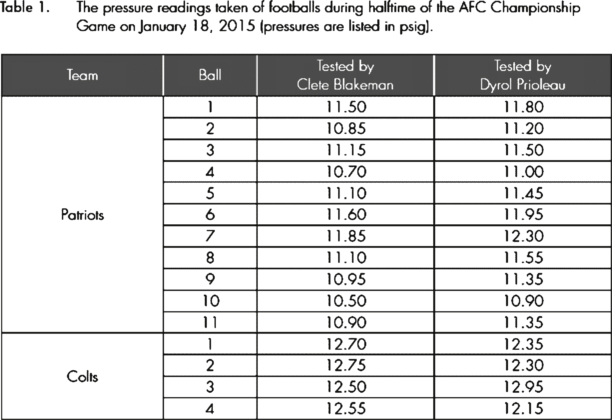
Table 1
Replication of key results in Wells report Table A-2, A-4, A-6, and A-8
| 1 | 2 | 3 | 4 | |
| α | 0.47 | 0.47 | 0.47 | 0.53 |
| (t-value) | (3.28) | (3.28) | (3.28) | (3.19) |
| β | 0.73 | 0.73 | 0.73 | 0.67 |
| (t-value) | (4.40) | (4.40) | (4.40) | (3.54) |
| Observations | 30 | 30 | 30 | 30 |
| R-squared | 0.41 | 0.41 | 0.41 | 0.33 |
Table 2
Key result in Wells report Table A-6 for different gauge scenarios
| 1 | 2 | 3 | 4 | |
| α | 0.37 | 0.37 | 0.77 | 0.77 |
| (t-value) | (2.83) | (2.83) | (5.90) | (5.90) |
| β | 0.63 | 1.03 | 0.23 | 0.63 |
| (t-value) | (4.16) | (6.79) | (1.53) | (4.16) |
| Observations | 30 | 30 | 30 | 30 |
| R-squared | 0.41 | 0.62 | 0.08 | 0.39 |
Table 3
Key result in Wells report Table A-6 for different gauge scenarios with timing controls
| 1 | 2 | 3 | 4 | |
| α | 0.29 | 0.29 | 0.69 | 0.69 |
| (t-value) | (0.88) | (0.88) | (2.11) | (2.11) |
| β | 0.57 | 0.97 | 0.17 | 0.57 |
| (t-value) | (1.54) | (2.63) | (0.46) | (1.54) |
| Timing Controls Observations | X 3 | X 3 | X 3 | X 3 |
| R-squared | 0.41 | 0.64 | 0.11 | 0.41 |


