
Analyzing the pace of play in golf
Abstract
We develop performance approximations that can help manage the pace of play in golf. In previous work we developed a stochastic model of successive groups of golfers playing on an 18-hole golf course and derived expressions for the capacity (maximum possible throughput) of each hole and the golf course as a whole. That model captures the realistic feature that, on most holes, more than one group can be playing at the same time, with precedence constraints. We now facilitate further performance analysis with that model by developing two new approximations. First, we develop an approximation involving a series of conventional single-server queues, without precedence constraints. The key idea is to use the times between successive departures on a fully loaded hole as aggregate service times in the new model. Second, we apply established heavy-traffic limits for a series of conventional queues to develop explicit approximation formulas for the mean and variance of the time required for group n to play the entire course, as a function of n. We conduct simulation experiments showing that both approximations are effective. We show how these formulas can help design and manage a golf course.
1Introduction
We apply stochastic models and computer simulation to develop performance formulas to help improve the design and management of golf courses. These formulas can help specify the constant interval between successive tee times (start times) for successive groups of golfers and the total number of groups that should be scheduled to play each day. They can can help balance the desire to put more golfers on the course in order to maximize the use of a valuable resource (and earn more revenue) and the desire to put fewer golfers on the course in order provide a good experience for the golfers by keeping delays low, and not exceeding the widely accepted standard of a four-hour round.
Our work builds on Whitt (2015), in which a stochastic model of group play on each hole of the golf course was developed, allowing multiple groups to be playing on the each hole with precedence constraints, and having random group stage playing times on each hole as primitives. The capacity (maximum possible throughput) was determined for each hole and thus the golf course as a whole. Earlier work modeling and simulating the play of golf was done by Kimes and Schruben (2002), Tiger and Salzer (2004) and Riccio (2012, 2013).
We develop approximations for the model in Whitt (2015) and apply them to develop explicit performance formulas. Our main contributions are (i) an approximating model involving conventional single-server queues, without precedence constraints, and (ii) an approximation formula for the expected value of the course sojourn time (the time for group n to play on the entire course), i.e.,
(1)
Approximation (1) is intended for the common case in which (i) the course is heavily loaded, with management being challenged to meet demand, and (ii) the course is balanced, in that the pace of play is not dominated by a few bottleneck holes. Underlying approximation (1) is previous mathematical analysis of heavily loaded networks of conventional single-server queues in series in Iglehart and Whitt (1970a, b), Harrison and Reiman(1981), Glynn and Whitt(1991) and Greenberg et al. (1993), but further work has to be done to bring that literature to bear on this problem, because group play on each hole is affected strongly by the precedence constraints, which are not part of conventional queueing models.
Figure 1 summarizes our results. It shows three estimates of the expected sojourn times E [V18,n] in the critically loaded case with A = 0. (For a precise definition of V18,n, see (11).) The results of a detailed simulation are shown by the circles; the solid line is a least-squares fit of the function
Detailed modeling can produce concrete analogs of approximation (1), but even without such modeling, formula (1) may be fit to data in order to help understand the relation between delays on the golf course and the primary controls: the tee intervals and the number of groups allowed to play. Formula (1) shows the non-obvious way that the mean sojourn time for group n should grow with n.
Here is how this paper is organized: In §2 we describe how groups of golfers play on a golf course. In §3 we review the stochastic model introduced in Whitt (2015) with random stage playing times as the basic primitives. In §4 we elaborate upon approximation 1 and explain Fig. 1 there. In §5 we show how approximation 1 can be applied to gain insight into the design and management of a golf course. In §6 we indicate how the model primitives (the stage-playing-time distributions) can be estimated from data, and how the stochastic model can be constructed and tested.
The remaining sections are devoted to developing and evaluating the two main approximations. In §7 we derive (1). In §7.1 we propose the new approximation of group play on a single hole by a conventional single-server queue, without precedence constraints. In §7.2 we apply that approximation to derive (1). In §8 we report results of simulation experiments testing the approximations. We draw conclusionsin §9.
2Group play on golf courses
Golf is typically played by small groups (e.g., four) golfers playing 18 (or sometimes 9) holes, usually maintaining the order of the group start (tee) times on the first hole. Each successive group has a scheduled tee time on the first hole, and starts thereafter at the first opportunity. Groups continue from hole to hole, stopping only to wait for the group in front. In practice, the first-come first-served (FCFS) order may be occasionally broken to cope with slow groups. For example, “rangers” may drive around the course in carts to speed-up or remove slow groups. However, we will not consider such modifications here.
There are three types of holes on a golf course: par 3, par 4 and par 5. The goal in golf is to put the ball into the hole on the green using as few strokes (shots) as possible. A hole is rated par 4 because good play should require four shots: one from the tee, one from the fairway and two more to clear the green (put it in the hole on the green). A “birdie” (“eagle”) is earned on the hole for scoring one (two) under par, while a “bogey” (“double bogey”) is earned for scoring one (two) over par. Usually, the par value of a hole is higher when the length of the hole is longer. A typical 18-hole golf course has 12 par-4 holes, 3 par-3 holes, and 3 par-5 holes, arranged in varied ways.
We will analyze the pace of play from the perspective of queueing theory and the theory of industrial production lines. Thus, we regard the play of successive groups on a golf course as the flow of successive “jobs” through a series of 18 queues in series, with unlimited waiting space at each queue and a FCFS service discipline. However, there is a serious complication, because more than one group can be playing at the same time on many of the holes, but with precedence constraints. Typically, two groups can be playing on a par-4 hole at the same time, while three groups can be playing on a par-5 hole at the same time. A conventional par-3 hole is more elementary because only one group can play on it at the same time, but there also is the modified par-3 hole “with wave-up,” which allows two groups to play at the same time there too, while still maintaining the group order determined by their scheduled tee times on the first hole.
To explain in greater detail, we describe the steps of group play on a par-4 hole. There are five steps, each of which must be completed before the group moves on to the next step. These five steps can be diagrammed as
(2)
The first step T is the tee shot (one for each member of the group); the second step W1 is walking up to the balls on the fairway; the third step F is the fairway shot; the fourth step W2 is walking up to the balls on or near the green; the fifth and final step G is clearing the green, which may involve one or more approach shots and one or more shots (putts) on the green for each player in the group. Each step must be completed before the group proceeds to the next step.
This natural characterization of group play closely follows previous simulation models; e.g., see the single-hole bottleneck model on p. 32 of Riccio (2013). However, as in Whitt (2015), we go beyond that direct representation by doing additional aggregation. In particular, we do not directly model the play of each golfer in the group and we also do not directly model the performance of each individual step. Instead, we aggregate the five steps into three stages, which are important to capture the way successive groups interact while playing the hole. The three stages are:
(3)
The precedence constraints follow common conventions in golf. Assuming an empty system initially, the first group can do all the stages, one after another without constraint. However, for n ≥ 1, group n + 1 cannot start stage 1 until both group n + 1 arrives at the tee and group n has completed stage 2, i.e., has cleared the fairway. Similarly, for n ≥ 1, group n + 1 cannot start on stage 2 until both group n + 1 is ready to begin there and group n has completed stage 3, i.e., cleared the green. These rules allow two groups to be playing on a par-4 hole simultaneously, but under those specified constraints. We may have groups n and n + 1 on the course simultaneously for all n. That is, group n may first be on the course at the same time as group n - 1 (who is ahead), but then later be on the course at the same time as group n + 1 (who is behind). The groups remain in their original order, but successive groups interact on the hole. The group in front can cause extra delay for the one behind.
A par-3 hole without the extra wave-up rule is more elementary. There are three steps for group play on a par-3 hole, with or without wave-up: T → W → G.The first step T is hitting shots off the tee; the second step W is walking to the green, possibly including approach shots; and the third step G is putting on the green. In this case we identify the stages with steps, but speak of stages, to be consistent with par-4.
Even though the par-3 holes are shorter, they often tend to be the bottlenecks because it tends to take longer for successive groups to clear the green. This can be attributed to the fact that only one group is allowed to play at the same time on a standard par-3 hole. (This is explained mathematically by Corollary 3 of Whitt (2015).) The wave-up rule is intended to reduce the expected time between successive groups clearing the green, and thus increase the capacity of par-3 holes.
The wave-up rule (only for par-3 holes) stipulates that, after a group has hit its tee shots and walked up to their balls near the green, they should wait before clearing the green until the following group hits its tee shots, provided that the following group has already arrived and is ready to play. If the following group has not yet arrived at the hole, then the current group immediately starts stage 3. The following group then cannot start play on the hole until after the current group completes stage 3 and departs.
The longest holes are the par-5 holes. On a typical par-5 hole, three groups can be playing simultaneously. For a par-5 hole, we identify seven steps instead of the five steps for a par-4 hole and the three steps of a par-3 hole. There now are two fairway shots instead of only one and three walking steps instead of only two. These seven steps can be grouped into five stages, as opposed to three for a par-4 hole:
Assuming an empty system initially, the first group can do all the stages, one after another without constraint. However, for n ≥ 2, group n cannot start stage 1 until both group n arrives at the tee and group n - 1 has completed stage 2, i.e., has completed its fairway shots (completed F1). Similarly, for n ≥ 2, group n cannot start stage 2 until both group n arrives at stage 2 and group n - 1 has completed stage 4, i.e., has cleared the second fairway shot (completed F2). After completing stage 2, each group may go right on to stage 3. for n ≥ 2, group n cannot start stage 4 until both group n arrives at stage 4 and group n - 1 has completed stage 5, i.e., has cleared the green (completed (W3, G)). After completing stage 4, each group may go right on to stage 5.
3A Stochastic model of group play
3.1Random stage playing times
In order to represent the inevitable variability in the play of actual golfers, stochastic models of group play on each of the four hole types (P3, P3WU, P4 and P5) were developed in Whitt (2015) by focusing on the stages instead of the steps. For each of the hole types, the time required for group n to complete stage i was modeled as a nonnegative random variables Si,n. As a regularity condition, these random stage playing times (for the group) were assumed to be mutually independent, having distributions that depend only on the hole type and the stage number.
We envision this model being carefully fit to data on group play on golf courses, but that is not done here. (We indicate how that fitting can be done in §6.) Instead, we use the parametric framework introduced in §4 of Whitt (2015) to develop the performance formulas and substantiate them with simulation here. Several parametric distributions of the stage playing times Si were introduced. The most promising of these is a symmetric triangular distribution, which is appealing to capture the usual relatively low variability. An additional modification is introduced to allow for occasional lost balls. This produces tractable models of the triple (S1, S2, S3) for a P4 hole depending on a 5-tuple of parameter values (m, r, a, p, L), where each parameter captures a separate property of the model; see Example 3 of Whitt (2015). In particular, the three random variables Si are assumed to be independent and are given symmetric triangular distributions on the intervals [mi - a, mi + a]. Further simplification is obtained by assuming that the mean values are related by m1 = m3 = m2/r = m. Thus S1 is distributed the same as S3, both having mean m, while E [S2] = rm, so that the ratio E [S2]/E [S1] = r can be controlled separately. (This structure draws on p. 94 of Riccio (2012) and p. 32 of Riccio (2013).) The variability of the three random variables Si is specified by the single parameter a. We then assume that lost balls occur only on the first stage (including the tee shots) of each hole, with that happening on any hole with probability p and leading to a fixed large time L for stage 1 (corresponding to a maximum allowed delay). Thus the parameter pair (p, L) captures rare longer delays.
3.2Recursions for each hole
To illustrate, we describe the stochastic model for a P4 hole in detail. Let An be the arrival time of the nth group at the tee of this hole on the golf course. Let Si,n be the time required for group n to complete stage i, 1 ≤ i ≤ 3; these are the stage playing times. With the assumptions above, {Si,n : n ≥ 1} for1 ≤ i ≤ 3 are three independent sequences of independent and identically distributed (i.i.d.) random variables, with distributions that depend on i.
Let Bn be the time that group n starts playing on this hole, i.e., the instant when one of the group goes into the tee box. Let Tn be the time that group n completes stage 1, including the tee and the following walk; let Fn be the time that group n completes stage 2, its shots on the fairway; and let Gn be the time that group n completes stage 3, and clears the green.
A concise mathematical representation is given by the recursion
(4)
3.3Performance measures
Associated performance measures for group n on the given hole are: the waiting time (before starting play on the hole), Wn ≡ Bn - An; the playing time (the total time group n is actively playing this hole, possibly including some waiting there), Xn ≡ Gn - Bn; and the sojourn time (the total time spent by group n at the hole, waiting plus playing), Un ≡ Gn - An = Wn + Xn. Let
A main contribution of Whitt (2015) was determining the maximum throughput for each hole. We start by defining the throughput here and later in §3.4 define the maximum throughput. For the golf course, the definition of throughput is complicated because the course starts empty each day and gets more congested throughout the day, until new groups no longer are allowed to start. However, the rate groups complete play may rapidly approach a limit, even if the system is overloaded. That limit is taken as the defining quantity.
The random cycle time (for group n on the given hole) is defined as
(5)
(6)
The typical case (in a mathematical model with an unlimited number of i.i.d. groups) is to have
(7)
We define the random throughput rate for the first n groups as
(8)
(9)
We define other average performance measures just like (6) and (8). For example, the average sojourn time, i.e., the average time spent at the hole per group (among the first n groups) is
(10)
These models for individual holes can be combined to obtain corresponding models for the full golf course for any combination of holes. In the model description, we add a subscript k for the hole number to go with the subscript n for the group number. We link the holes together by letting Ak+1,n = Gk,n; i.e., we let the arrival time of group n at hole k + 1 equal the completion time of group n at hole k. In doing so, we ignore the travel time between holes, but that could be added as well if it is deemed important. Thus, the model fully specifies group play on a golf course, e.g., it can be used to perform computer simulations, given any specification of the hole types and the stage playing time distributions on each hole.
With these conventions, we are primarily interested in the mean sojourn time E [Vk,n], the mean sojourn time of group n on the first k holes, where
(11)
3.4The maximum throughput on each hole
An important contribution of Whitt (2015) is determining the capacity of each hole for the stochastic model defined above. The capacity of a hole is defined as the maximum possible throughput rate given a fully loaded hole, i.e., given that new groups are always available to start play as soon as possible. The capacity of the golf course then is the minimum of the capacities of the individual holes on the course.
For each hole type, when the hole is fully loaded, the random cycle times
(12)
The distribution of the critical cycle time Y was characterized for each of the hole types. For example, for a P4 hole, Theorem 1 of Whitt (2015) shows that
(13)
Another key random variable describing the performance of a fully loaded hole in steady state (for group n as n gets large) is the critical playing time X; it is the random time it takes a group to play the hole, i.e.,
(14)
Theorem 7 of Whitt (2015) shows that for a P3WU hole
(15)
4The sojourn time approximation formulas
We now exhibit approximation formulas for the mean and standard deviation of the sojourn time on the entire course for group n as a function of n, and elaborate upon (1) and Fig. 1. In §4.1 we relate the constant intervals between tee times and the maximum throughput on each hole to the traffic intensity. In §4.2 we review the key assumptions underlying the approximation formulas. In §4.3 we give the full formulas and in §4.4 we explain Fig. 1. We derive the approximation formulas in §7.
4.1From tee times to the traffic intensity
To put this problem in standard queueing terminology, let the arrival rate to the first hole and the course be defined as the reciprocal of the constant interval between tee times on the first hole, i.e.,
(16)
For any given arrival rate λk on hole k, there is an associated throughput rate or departure rateθk ≡ θk (λk), representing the long-run rate of groups completing play on hole k, which becomes the arrival rate on hole k + 1. The model we use is consistent with the basic throughput formula
(17)
When we consider a sequence of queues, we must consider the maximum throughput through all previous queues. Thus,
(18)
(19)
In queueing theory it is common to focus on a dimensionless measure of the arrival rate called the traffic intensity ρ, but in the present context it requires knowing the maximum possible throughput rate. The traffic intensity is obtained by dividing the arrival rate by the maximum possible throughput rate. For hole k in isolation, the definition is
(20)
(21)
The full golf course tends to be underloaded, critically loaded or overloaded as ρ < 1, ρ = 1 and ρ > 1. By the equations above, once the maximum possible throughput has been determined, the choice of any one of ρ, λ or Δ implies a corresponding choice for all three. Since expressions of the maximum throughput have been developed, we can work with the traffic intensities ρk in (20),
4.2Key assumptions
A golf course is said to be balanced if the maximum throughput on each hole coincides with the overall maximum throughput, i.e., if
(22)
Given that we do have a balanced course, which implies that the mean critical cycle times E [Y] are identical for all holes, to approximate the expected waiting times at all the queues as a function of n, we made a further approximation: We consider a more stylized model by assuming that all holes are identical P4 holes. This assumption seems reasonable, provided that the course is balanced, because usually 12 of the 18 holes are P4 holes. Work is in progress to carefully evaluate the extent to which this stylized model captures the essential performance of typical balanced courses, having the usual variety of holes.
To many, especially experience golfers, this approximation assumption may seem counterintuitive, because from experience they know that the playing time tends to increase significantly as the par value increases. However, we are using the identical-P4 approximation only to approximate the random critical cycle time Y, and the associated expected waiting times. We include separate approximations of the expected playing times, which depend on the hole type, as well as the common random critical cycle time Y. Indeed, simulations of the models in Whitt (2015) confirm that the playing times on P3WU, P4 and P5 holes can be very different even when E [Y] is the same.
4.3Approximation for the golf course model
As we will explain in §7.2, the approximation (1) is based on a heavy-traffic limit for a critically loaded network of single-server queues. That means that a variant of approximation formula (1) can be justifiedfor a series network of conventional single-server queues asymptotically as n→ ∞, provided that ρ ≥ 1. Indeed, for the application of approximation (1), we assume that ρ ≥ 1. The formula for ρ = 1 may be a useful approximation if ρ is approximately 1, but we do not intend for approximation (1) to be applied with ρ < 1. The scaling in the heavy-traffic limit (given in (37)) implies that the error is asymptotically negligible compared to
Our heavy-traffic approximation for the mean sojourn time of group n on a balanced golf course with ρ ≥ 1 is (1) with the constants given by
(23)
The leading constant A in (1) depends only on the constant tee interval Δ and the mean critical cycle time E [Y], and so is robust for the fully loaded case with ρ ≥ 1. On the other hand, the constant B depends on both the mean E [Y] and the scv
The variability in the stage playing times Si has a significant impact on the mean critical cycle time E [Y] as well as its variance. Such variability might arise if (i) groups of widely varying skills are allowed to play the course, or if (ii) the size of groups is allowed to be quite variable, or if (iii) groups of golfers are allowed to either walk the course or ride in carts. Now we see that the mean and variability of Y both have a significant impact on the mean time for a group to play the course, E [V18,n].
The core of the constant C in (23) is the first term, which is the sum of the mean playing times on each hole, assuming that they are all fully loaded. This formula allows these mean hole playing times to vary from hole to hole. For a network of identical P4 holes, the first term reduces to
We also propose an approximation for the standard deviation of the total sojourn time based on the same heavy-traffic limit.
(24)
4.4The simulation experiment leading to Fig. 1
We now introduce the specific model used to generate Fig. 1 in §1. It is a stylized model containing 18 identical P4 holes in series with ρ = 1, which makes A = 0 in the approximation (1). We let all stage playing times have the tri + LB triangular distribution modified to allow for lost balls (only from the tee, i.e., on the first stage of each hole) introduced in §(3.1). We let the parameter vector be (m, a, r, p, L) = (4, 1.5, 0.5, 0.05, 8). With these parameters, the critical cycle time Y (the interval between successive groups completing play on a fully loaded hole) has mean E [Y] =6.5325, but for the variance we need to correct a minor error in Whitt (2015).
Remark 4.1. (correction) There is a minor error in the formula for
Applying Remark 4.1 without using the
Figure 1 in §1 shows the estimated expected sojourn times E [V18,n] over the 18-hole course as a function of the group number n, based on simulation experiments. The simulations are based on 2000 independent replications. This consistently makes the half-width of 95% confidence intervals less than 5% of the estimated means and 10% of the estimated standard deviations. The smooth plot of the simulation mean values for successive groups is further evidence of the simulation precision.
Note that these parameter values appear to be reasonable. The expected time for the first group to play the course is 18 × 10.2 = 183.6 minutes or about three hours. We see that the expected times to play the course (from tee time on the first hole to clearing the green on hole 18) for each of the first 60 groups is under the target four hours, but the expected times for later groups are longer. The expected time for group 100 is about 4.5 hours. And this is for a fairly idealized model (what we take to be a good case). In particular, here we have 18 identical P4 holes in series.
As shown in Fig. 1, for ρ = 1.0, the heavy-traffic approximation in (1) and (23) becomes
Note that we apply the heavy-traffic approximation in (1) to obtain the functional form
However, the approximation for the constant C is not so well supported, which may be explained by the complexity of the model, including the exceptional experience of the first group on all holes. For n = 100, the heavy-traffic approximation underestimates the simulation estimate by about 5; indeed, the heavy-traffic approximation falls on top of the simulation estimate if we increase C to 186. As in all heavy-traffic approximations, there is room for refinements, e.g., see Whitt (1982).
5Application to manage the pace of play
We now show how the approximate performance formula for the mean sojourn time E [V18,n] in (1) and (23) can be applied in the design of a golf course. In particular, we show how it can be used to help determine the number of groups that should be allowed to play each day, and thus the (assumed constant) interval between tee times Δ, as a function of the key model parameters and specified performance constraints. For this analysis, we consider the special case of a course that contains 18 identical P4 holes.
We formulate an optimization problem, aiming to maximize the number n of groups the play each day for specified model parameters
(25)
For example, if we were to aim for 4-hour rounds over a 14-hour day, then we would have γ = 240 minutes and τ = 840 minutes. The tee times could then be restricted to the interval [0, τ - γ] = [0, 600] minutes.
From (1) and (23), we have for ρ ≥ 1 the following functions of the model parameters and n:
(26)
(27)
Since feasible numbers of groups must be integer, we round down to the nearest integer; let ⌊x⌋ be the floor function, the greatest integer less than or equal to x.
Theorem 5.1. (optimal solution) The function V (ρ, n) in (26) is increasing in n and ρ, while the function G (ρ, n) is increasing in n and independent of ρ, provided that n ≥ 1 and ρ ≥ 1. Hence, if there is an optimal solution, then one of the two constraints must be satisfied as an equality. If the first constraint on V is binding, then the optimal decision variables are
(28)
(29)
Proof. First, suppose that the first constraint involving V is binding. Since V (ρ, n) is increasing in both ρ and n, in order to achieve the largest value of n, it suffices to restrict attention to the smallest value of ρ, yielding
Theorem 5.1 implies that it suffices to focus on ρ = 1 in the optimization problem. This should be consistent with intuition, because it is impossible to achieve throughput faster than the bottleneck rate achieved at ρ = 1. Since we achieve ρ = 1 by setting Δ = E [Y], we see the importance of determining E [Y].
We say that a golf course design is efficient if the two constraints in (25) are both binding at the optimal solution. An efficient design has the advantage that it should not be necessary to increase throughput at the expense of golfer experience (excessive times to play a round). At the same time, it should not be necessary to restrict the throughput in order to achieve a target bound on the time to play a round. Efficiency depends on the constraint limits γ and τ as well as the model parameters. The following elementary result characterizes an efficient design.
Theorem 5.2. (efficient design) An efficient design for (γ, τ) occurs if and only if there is an nef such that
(30)
(31)
Example 5.1.To illustrate Theorem 5.1, supposethat τ = 840, γ = 240, E [Y] =6, E [S3] =4 and
To illustrate Theorem 5.2, observe that, since
(32)
6Data collection and model fitting
We envision the stochastic model of group play discussed above being used either to design a new golf course or to improve the pace of play on an existing golf course. In this section we discuss the required data collection in order to fit the model.
6.1Measuring the stage playing times
The primitives of the model are the stage playing times of successive groups. Given a specification of the actual stage playing times of all groups on all holes, the recursions in Whitt (2015), such as the par-4 recursion in (4) here, produce a specification of the resulting play of all groups on all holes. (The major exception is that we have ignored any delays spent walking after completing play on one hole to the tee at the next hole. We also assumed that the groups maintain their order of play.) The implication is that we can calculate the resulting performance descriptions for any number of groups on any day for any specification of the stage playing times and scheduled tee times. Moreover, we can apply simulation to estimate the expected performance descriptions for any number of groups on any day for any stochastic specification of the stage playing times and tee times.
The stage playing times for each hole in turn can be determined from the times each golfer in the group makes their shots on that hole. For example, on a par-4 hole, there are five steps and three stages, as shown in (2) and (3). Play starts when the first golfer in the group goes to the tee. There are then three stage playing times, with S1 corresponding to (T, W1), S2 to F and S3 corresponding to (W2, G). The first time S1 can be defined as the time between the instant the first golfer in the group hits a tee shot until the first golfer in the group hits a fairway shot; the second time S2 can be defined as the time between the instant the first golfer in the group hits a fairway shot until the instant that the last golfer in the group hits a fairway shot; and the third time S3 can be defined as the time between the instant the last golfer in the group hits a fairway shot until the instant that the last golfer in the group hits a shot on the hole (most likely a putt on the green). Thus all the stage playing times can be extracted from the times at which each golfer hits the ball. It suffices to record the times of all golf shots of the group.
The stage playing times can also be measured according to the locations of the golfers in the group. The first time S1 can be defined as the time between the instant that the first golfer in the group enters the tee box until the instant that the last golfer in the group passes an initial target crossing point in the fairway (e.g., 100 yards from the tee); the second time S2 can be defined as the time between the instant that the last golfer in the group passes an initial target crossing point in the fairway (e.g., 100 yards from the tee) until the instant that the last golfer passes a second target crossing point on the fairway (e.g., 250 yards from the tee); the third time S3 can be defined as the time between the instant that the last golfer passes the second target crossing point on the fairway (e.g., 250 yards from the tee) until the instant that the last golfer leaves the green (after all golfers have completed play on the hole). There could be difficulties in setting consistently appropriate initial and second crossing points on the fairway. This method could lead to errors if all golfers do not pass the initial crossing point after their tee shot or if they all do not pass the second crossing point after their fairway shot.
The ideal approach is to have the shot timers or GPS player location identifiers routinely incorporated on the golf course, so that data can be collected automatically and systematically. Alternatively, observers can conduct sampling. Golf courses could help groups of golfers self-regulate by exploiting modern technology to make timing information available throughout the golf course. The need has long been recognized, as can be seen from the many efforts over the years to address the pace-of-play problem without the latest technology, e.g., Wolfe (1980), Nixon (1996) and Probert (2000).
6.2Constructing the stochastic model
To construct the associated stochastic model of group play over the course, we need to estimate the probability distribution of each stage playing time on each hole, which can be characterized by its cumulative distribution function (cdf) F. For each stage playing time on each hole, that is naturally done by constructing the empirical cumulative distribution function (ecdf). Given n observations Zi, 1 ≤ i ≤ n, of one stage playing time with cdf F, the ecdf is
(33)
In our examples, we have used symmetric triangular distributions and exponential distributions for the stage-playing-time cdf’s, but these are just hypothetical distributions to illustrate the key concepts, with the triangular distribution being roughly appropriate to characterize the anticipated relatively low variability. As illustrated by Corollary 2 and §4 of Whitt (2015), these distributions are convenient for mathematically calculating the associated critical cycle time Y, as in (13), and critical playing time, as in (14). More generally, for any stage-playing-time distributions, the associated distributions of Y and X can be estimated by simulation, using the formulas and recursions.
For quick rough estimates with very limited data, the symmetric triangular distribution is convenient because it requires specifying only the minimum and maximum values. More generally, with limited data or only rough intuitive judgment, it is common to use three-point estimation, using a smooth beta or PERT distribution based on the most likely value (mode) in addition to the estimated minimum and maximum values. That smooth three-point estimation is likely to provide a better fit than the symmetric triangular distribution, but we would no longer have the relatively simple formulas in §4.2 of Whitt (2015).
6.3Testing the stochastic model: Detecting slow groups
The stage playing times are natural model primitives because, unlike the sojourn, waiting and playing times on the hole or on the entire course, they are performance measures that do not depend on the play of other groups. Thus the stage playing times serve to characterize the group play, and are thus appropriate for model input.
In the stochastic model, a key modeling assumption we make is that the stage playing times are stochastically independent over different groups and different holes. The stage-playing-time cdf’s are allowed (indeed, are deliberately chosen) to vary from stage to stage and from hole to hole, but the random times are assumed to be stochastically independent; i.e., they are assumed to be uncorrelated.
An important (and familiar) way that this independence condition can be violated is by having some extremely slow groups. Without slow groups, our model allows any group to occasionally be slow on any hole, e.g., due to a rare lost ball. However, slow groups are different, because they are consistently slow on all holes. Since all their stage playing times tend to be larger than average, this seriously violates our independence assumption.
With data, it is thus natural to perform statistical tests of the assumed independence, aiming to detect correlations among the playing times. A convenient statistical test of our independence assumption is to estimate the mean and variance of the sum of the stage playing times over all stages and holes, for each group. We will thus have one sum for each group. It should be easy to detect exceptionally slow groups, because they will produce outliers (extremely large values) of these sums of stage playing times.
But it is also not hard to do more careful analysis. Under the independence assumption, the variance of the sum will be the sum of the variances of the individual stage playing times, and the total will approximately have a Gaussian distribution (by virtue of the central limit theorem). On the other hand, with slow groups, there will be positive correlations, making the variance of the sum much larger. Thus, a practical statistical test of the independence hypothesis is easily carried out; i.e., we perform a standard statistical test to determine if the n sums can be regarded as i.i.d. Gaussian with the hypothetical mean and variance (under the independence hypothesis). Clearly, the independence assumption is likely to be more reasonable when the skill level of golfers on the course does not vary too greatly. Otherwise, the impact of slow groups can be so great that golf courses recognize that they have to take measures to address the problem.
6.4Seeing if the course is balanced
The relatively simple performance descriptions in this paper depend on the course being roughly balanced, which means that the maximum possible throughput on each hole is about the same for all holes. In our examples we have used identical P4 holes, so that the course is clearly balanced, but we have confirmed in simulations (to be reported in a sequel paper) that the courses can have all the usual holes, with different parameters for each hole type, provided that the expected critical cycle times E [Y] are approximately the same on all holes. This is an important conclusion that should be applied when designing golfcourses.
In practice, we can test whether or not a course is balanced in at least two ways. First, if we estimate the stage-playing-time cdf’s on each hole, then we can estimate the mean critical cycle time E [Y] for each hole. The course is balanced if these are approximately the same for all holes.
Second, we can also detect unbalanced courses by observing unusually long waiting times (before starting to play on a hole) for the last groups to play at the most heavily congested holes. For a balanced critically loaded course, the waiting times tend to gradually build up over successive groups and gradually decrease over each successive hole. For an unbalanced course, the waiting times at a few heavily congested holes tend to dominate the waiting times at other holes.
7Derivation of the approximation formulas
In this section we derive the approximation formulas for the mean total sojourn time in (1) and (23) and for the standard deviation in (24). We have placed this section toward the end of the paper, because it involves quite complicated and sophisticated queueing theory. We emphasize that this is far from a conventional application of queueing theory. The golf course tends not to operate in steady state. Instead, it is a heavily loaded system that starts out empty each day. Moreover, there are the precedence constraints associated with more than one group playing on each hole at the same time.
In §7.1 we show how to approximate the group waiting times (before starting to play) on each of the holes by the waiting times in associated conventional G/GI/1 single-server models with unlimited waiting space, the FCFS discipline, the given arrival process of groups to the hole and i.i.d. (aggregate) service times; i.e, without the precedence constraints. In §7.2 we then apply established heavy-traffic limits for a series of identical conventional queues to develop the final approximation. In §7.2.2 we show how we obtain the final formulas for the golf course.
7.1An approximation without precedence constraints
In order to apply conventional queueing theory to develop approximations for the sojourn time on the course, we now approximate the P3WU, P4 and P5 holes specified in §3 by conventional G/GI/1 single-server models with unlimited waiting space, the FCFS discipline, the given arrival process of groups to the hole and i.i.d. (aggregate) service times. In this case, there also are some exceptional initial conditions: (i) the first customer arrives at time 0 instead of after an interarrival times and (ii) the first customer has an exceptional service time. These features will require some adjustment in the approximations. The main point is: In these approximating models, only one group is being served at a time, ignoring all other groups. The approximation is avoiding the precedence constraints.
7.1.1The approximating conventional single-server queue
We now approximate each individual hole by a conventional G/GI/1 single-server queue, which has no precedence constraints. By “conventional G/GI/1 single-server queue,” we mean a single-server queue with unlimited waiting space, the FCFS service discipline, the given arrival process and i.i.d. service times with a general distribution (which are independent of the arrival process). In a conventional single-server queue, whenever the server remains busy, the intervals between successive departures are the exogenously defined service times. Thus in our approximation we let the new aggregate service times be i.i.d. versions of the critical random cycle times, distributed as Y in §3.4. We should only expect this approximation to be effective when the hole is heavily loaded, but that is the important case that we consider.
Moreover, we only use this approximating aggregate service time model to generate approximations for the waiting times before beginning service, i.e, for Wn ≡ Bn - An. Since the actual time spent playing on the hole Xn tends to be larger than Yn, to approximate the sojourn time on the hole we use the approximation
(34)
For a P4 hole, approximation (34), together with (13) and (14), implies that
(35)
7.1.2The classical recursion
Thus, for each hole type, the approximating G/GI/1 model is specified by the sequence of arrival times {An : n ≥ 1} and the sequence of mutually independent service times {Yn : n ≥ 1}, where
(36)
As indicated above, there is an exceptional first service time at each hole. We remark that there is a literature on queues with exceptional first service, which can be traced from citations to the early paper Welch (1964), but that literature focuses on queues in which the first service time of every busy period is exceptional. In contrast, here only the very first group has a different service time.
7.2The heavy-traffic approximation for the series network
We first consider a series of i.i.d. standard G/GI/1 queues, where the first queue has a deterministic arrival process and the service times are taken from 18 independent sequences of i.i.d. random variables distributed as Y(4), the critical P4 cycle time variable in (13). Then we show how to modify that approximation to obtain approximations for the mean and standard deviation of the total sojourn time of each group in the general (critically loaded and balanced) golf course model.
7.2.1Heavy-traffic limit for the standard model
Let
(37)
(38)
It remains to evaluate the distribution of the random variable
(39)
(40)
(41)
Combining (38), (40) and (41), we obtain the approximations
(42)
7.2.2Extending the approximation to the golf course
To obtain the corresponding approximation for the sojourn time in the golf model, we need to include the sojourn time adjustment in §7.1.1. Since the expected playing time on hole k is E [Xk] instead of E [Y], we need to add E [Xk] - E [Yk] to the approximation for the mean
We subtract the constants B = 7.2σY in C in (23) to account for the shift from
For the standard deviation, there evidently is dependence among these stage playing times used in the adjustment. Hence, we advocate the simple approximation
(43)
8Simulation experiments
We now report results of additional simulation experiments conducted to evaluate the approximations.
8.1Simulation to test the conventional queue approximation
We first report the results of simulation experiments to test the approximation by conventional G/GI/1 single-server queues with i.i.d. service times distributed as the critical cycle time Y, proposed in §7.1.1. Again, the simulations are based on 2000 independent replications, which makes the half-width of 95% confidence intervals less than 5% of the estimated means and 10% of the estimated standard deviations.
8.1.1A single critically loaded P4 hole
We first consider the case of a single P4 hole that is critically loaded. The approximation yields a conventional D/GI/1 queue, with two modifications: the first customer arrives at time 0 and has an exceptional service time. Theorem 4.1 of Whitt (1972) gives a heavy-traffic limit for the mean waiting time in a GI/GI/1 queue as n→ ∞ when ρ = 1. For the D/GI/1 model with service time having variance
(44)
(45)
(46)
Figure 3 compares the heavy-traffic approximation in (46) to simulation estimates for the first P4 hole of the same tri + LB model used in Fig. 1 and a fitted function, which turns out to be
8.1.2A series of identical P4 holes
We next consider the case of identical P4 holes in series with different distributions for the stage playing time Si, 1 ≤ i ≤ 3. We report simulation results estimating the mean and standard deviation of the sojourn time of group n on hole k, Uk,n ≡ Gk,n - Ak,n, and of group n on the first k holes, Vk,n ≡ U1,n + ⋯ + Uk,n for the cases (k, n) = (10, 20) and (18, 100).
We find that the sojourn times over several holes tend to be approximately normally distributed, so that the mean and standard deviation serve to describe the entire distribution. Figs. 4 and 5 illustrate by showing the histogram of the sojourn times V10,20 for ρ = 0.9 (on the left) and ρ = 1.1 (on the right) estimated for the exact model in §3. (The approximation produces very similar plots.)
For our first experiment, we consider an all-exponential model with independent all-exponential stage playing times having means E [S1] = E [S3] =6, E [S2] =3. The interval between tee times is used to adjust the traffic intensity ρ. We perform the transient simulations for three values of the traffic intensity ρ, defined by ρ ≡ λE [Y]: 0.9, 1.0, and 1.1.
We give simulation estimates of the mean and standard deviation of these sojourn times Uk,20 for the exact and approximate models in Table 1 for holes h = 1, 2, 3, 6 and 10 and the total sojourn time V10,20. Overall, we see that the mean sojourn time may increase from k = 1 to k = 2 but then gradually declines thereafter; the standard deviations evidently decline only after k = 3. We see that the approximate model consistently overestimates the mean and standard deviation but not by too much. It overestimates the mean and standard deviation of V10,20 for ρ = 0.9 by 7% and 12%, respectively. Assuming approximate normality, as supported by Figs. 4 and 5, the half-width of 95% confidence intervals for the mean can be estimated directly from the results in each table by
We now focus on the different stage playing time distributions. In all cases the three distributions are given the same form and three means are m1 = m3 = 6 and m2 = 3. In addition to the exponential distribution, we consider the triangular distribution (tri (m, a)) for (m, r, a) = (6, 0.5, 3) and that same triangular distribution with the lost ball parameters (p, L) = (0.05, 12). As indicated in Whitt (2015), the means and variances of Y can readily be computed for each of these three cases. They are, respectively,
Table 2 gives simulation estimates of the mean and standard deviation of these sojourn times Uk,100 for the exact and approximate models for holesk = 1, 2, 3, 6, 10, 18 and the total sojourn time V18,100. These results are again based on 2000 independent replications. For the less variable triangular stage playing time distribution, the half-width of 95% confidence intervals is consistently less than 1% of the mean estimate and 5% of the standard deviation estimate.
Again, we see that the mean sojourn time may increase from k = 1 to k = 2 but then gradually declines thereafter; the standard deviations evidently decline only after k = 3. We see that the approximate model consistently overestimates the mean and standard deviation but not by too much. The values decrease going from exponential to triangular with lost balls, and then to triangular without lost balls, because the variability decreases dramatically. Thus, Table 2 illustrates the strong impact of variability on performance, so pervasive in queueing theory.
8.2Simulations to evaluate the approximation formulas
We now report the results of simulations to evaluate the approximation formulas developed in §4.
8.2.1The approximations for the standard series network
To evaluate the quality of the approximation in (42), we simulated the standard model with i.i.d. service times distributed as Y in (13) with traffic intensities ρ = 1.1, 1.0 and 0.9 for the stage playing time distributions in Table 2. The results are shown in Table 3. For ρ = 1.0, the approximations for the mean sojourn time of group 100 over 18 holes with the tri, tri + LB and exp stage service time distributions are, respectively, 3.9% high, 10.6% high and 3.7% high.
For the cases with ρ ≥ 1, Table 3 shows that (42) and (42) provide useful approximations for the mean E [V18,n] and standard deviation
Our main focus is on cases with ρ ≥ 1, but Table 3 also includes results for ρ = 0.9 to show what happens. Table 3 shows that there are no dramatic changes; we can obtain reasonable rough estimates for the mean values at ρ = 0.9 by subtracting the difference of the values at ρ = 1.1 and ρ = 1.0 from the value for ρ = 1.0. However, the approximations for ρ = 0.9 have a very different basis. For ρ < 1, we use a variation of the approximation for the steady-state mean from Whitt (1983). For the standard deviation, we draw on (42), assuming that
8.2.2The approximations for the golf course
We use simulation to evaluate the approximations for the mean in (1) and (23) and for the standard deviation in (42) and (43). The results are inTable 4.
Table 4 show that the HT approximation gives a useful approximation for the mean E [V18,n] and standard deviation SD [V18,n]. From Tables 3 and 4, we see that the errors in Table 4 are primarily due to the quality of the heavy-traffic approximation for the standard model in this setting.
9Conclusions
We have developed two new approximations for the stochastic model of group play on a golf course introduced in Whitt (2015). In §7.1 we developed the approximation involving conventional G/GI/1 single-server queues, without precedence constraints. In §4 we exploited that approximation plus established heavy-traffic limits for queues in series reviewed in §7.2 to develop approximation formulas for the mean and standard deviation of V18,n, the random time spent playing the course by group n, as a function of n. The approximation for the mean is given in (1) and (23), while the approximation for the standard deviation is given in (24). The full distribution is approximately Gaussian, as can be seen from Figs. 4 and 5.
The mathematical basis was an established heavy-traffic limit for a network of conventional single-server queues in series. In particular, we used Theorem 3.2 of Glynn and Whitt(1991), but also simulation experiments in Greenberg et al. (1993). As noted in those papers, the variability in the total sojourn time is impressively low. However, we mainly emphasize the formula for the mean in in (1) and (23). It goes beyond widespread golfer experience that the expected time to play a round increases the later you start by revealing the form of that increase. In §5 we showed how that mean formula can be used to help design and manage a golf course.
There are many remaining research problems. First, work is underway to see how well the approximations perform for balanced courses with the usual variety of holes; all the simulations reported here were for 18 identical par-4 holes. For the more general model with different hole types, we tentatively propose approximation (1) with the general approximation for C in (23), involving the mean stage playing times on the different holes, but some adjustments may be needed, because the distribution of the critical cycle time Y depends on the hole type, even if the mean values are the same for all holes (so that the course is indeed balanced). In general, we expect the general form
Much remains to be done investigating data from group play on golf courses, going beyond the initial study in Riccio (2014), as discussed in §6. To what extent are group tee times consistent with the assumed deterministic schedule? To what extent are group sojourn times and departure times consistent with the approximation in (1)? To what extent are golf courses underloaded, critically loaded or overloaded? To what extent are golf courses balanced or unbalanced? What are the actual stage playing time distributions? To what extent are stage playing times mutually independent?
In §6.3 we observed that one reason that the stage playing times may not be independent is that there may be exceptionally slow groups. If there are occasional slow groups, and these groups are allowed to play the course, then they can have a major impact, as observed in Riccio (2012, 2013). Such slow groups would make the mean and variance of stage playing times larger. Even more important, they would make the successive stage playing times highly dependent. How should slow groups be analyzed? How should slow groups be managed?
For balanced courses, to what extent are the designs efficient as defined in §5? When the courses are inefficient, is the throughput constraint the binding constraint, as in Example 5.1? For unbalanced courses, what are effective performance approximations?
Finally, it appears that the present approximations can be fruitfully applied in other systems with precedence constraints, which commonly occur in many service systems, e.g. Armony et al. (2015), Larson et al. (1993). That remains to be explored.
Acknowledgment
This research was begun while the first author was a student in the IEOR Department at Columbia University. We thank Lucius J. Riccio for suggesting this general line of research and for many helpful discussions.We thank MoonSoo Choi for his contributions to this work and the intended sequel simulation study of the performance of the usual golf courses with diverse hole types. The second author received support from NSF (NSF grants CMMI 1066372 and 1265070).
References
1 | Armony, M., Israelit, S., Mandelbaum, A., Marmor, Y., Tseytlin, Y., Yom-Tov, G., 2015. Patient flow in hospitals: A data-based queueing-science perspective, the Technion, Haifa, Israel. Stochastic Systems. DOI: 10.1214/14-SSY153 (published online) |
2 | Cooper RB(1982) Introduction to Queueing Theory2nd EditionNorth Holland Amsterdam |
3 | Glynn PW, Whitt W(1991) Departures from many queues in seriesAnnals of Applied Probability1: 4546572 |
4 | Greenberg AG, Schlunk O, Whitt W(1993) Using distributed-event parallel simulation to study many queues in seriesProbability in the Engineering and Informational Sciences7: 2159186 |
5 | Harrison JM, Reiman MI(1981) Reflected Brownian motion on an orthantAnnals of Probability9: 2302308 |
6 | Iglehart DL, Whitt W(1970) aMultiple channel queues in heavy traffic, I.Advances in Applied Probability2: 1150177 |
7 | Iglehart DL, Whitt W(1970) bMultiple channel queues in heavy traffic, II: Sequences, networks and batchesAdvances in Applied Probability2: 2355369 |
8 | Kimes S, Schruben L(2002) Golf revenue management: A study of tee time intervalsJournal of Revnue and Pricing Management1: 2111119 |
9 | Larson RC, Cahn MF, Shell MC(1993) Improving the New York arrest-to-arraignment systemInterfaces23: 17696 |
10 | Nixon R(1996) Golf course timer to alleviate slow playU. S. Patent5: 523985 |
11 | Probert CF(2000) Golf course pace of play tracking system and methodU. S. Patent6: 135893 |
12 | Riccio L(2012) Analyzing the pace of play in golf: The golf course as a factoryInternational Journal of Golf Science1: 90112 |
13 | Riccio L(2013) Golf’s Pace of Play BibleThe Three/ Golf Association45New York |
14 | Riccio, L., 2014. The status of pace of play in american golf, 31 page research paper on the Three/45 Golf Association web page: http://www.three45golf.org/ |
15 | Tiger A, Salzer S(2004) Daily play at a golf course: Using spreadsheet simulation to identify system constraintsINFORMS Transactions on Education4: 22835 |
16 | Welch PD(1964) On a generalized M/G/ queuing process in which the first customer of each busy period receives exceptional serviceOperations Research12: 5736752 |
17 | Whitt W(1972) Complements to heavy traffic limit theorems for the GI/G/ queueJournal of Applied Probability9: 1185191 |
18 | Whitt W(1982) Refining diffusion approximations for queuesOperations Research Letters1: 5165169 |
19 | Whitt W(1983) The queueing network analyzerBell System Technical Journal62: 927792815 |
20 | Whitt W(2015) The maximum throughput on a golf courseProduction and Operations Management24: 5685703 |
21 | Wolfe NT(1980) System and method of timing golfers on a golf courseU. S. Patent4: 303243 |
Figures and Tables
Fig.1
The heavy-traffic approximation in (1) (
![The heavy-traffic approximation in (1) (8.04n+181.6), developed in §4, and the two-parameter
fit to the simulation estimates (8.32n+182) compared to the simulation estimates of E [V18,n], the
expected time for group n to play all 18 holes, as a function of n, for a critically loaded golf course
model with identical par-4 holes, with all stage playing times having the triangular distribution, modified to
allow lost balls, with parameter five tuple (m, a, r, p, L) = (4, 1.5, 0.5, 0.05, 8.0), specified in §3.1.](https://ip.ios.semcs.net:443/media/jsa/2015/1-1/jsa-1-1-jsa0004/jsa-1-1-jsa0004-g001.jpg)
Fig.2
The histogram of the critical cycle time Y on a (fully loaded) par-4 hole, defined in (13), with all stage playing times having the triangular distribution, modified to allow lost balls, with parameter five tuple (m, a, r, p, L) = (4, 1.5, 0.5, 0.05, 8.0), specified in §3.1, estimated using simulation with a sample size of 105. The estimated mean and variance were E [Y] =6.535 and Var (Y) =1.249.
![The histogram of the critical cycle time Y on a (fully loaded) par-4 hole, defined in (13),
with all stage playing times having the triangular distribution,
modified to allow lost balls,
with parameter five tuple (m, a, r, p, L) = (4, 1.5, 0.5, 0.05, 8.0), specified in §3.1,
estimated using simulation with a sample size of 105. The estimated mean and variance were E [Y] =6.535
and Var (Y) =1.249.](https://ip.ios.semcs.net:443/media/jsa/2015/1-1/jsa-1-1-jsa0004/jsa-1-1-jsa0004-g002.jpg)
Fig.3
The heavy-traffic approximation (46) and a two-parameter fit to the simulation estimates (
![The heavy-traffic approximation (46) and a two-parameter fit to the simulation estimates (0.903n-0.777) compared to the simulation estimates of E [W1,n], the expected waiting time of group n on the
first hole (in minutes, before starting to play), as a function of n, for a P4 hole with ρ = 1, where all
stage playing times have the tri + LB distribution with parameter five tuple (m, a, r, p, L) = (4, 1.5, 0.5, 0.05, 8.0), reviewed in §3.1 (the same as in Fig. 1).](https://ip.ios.semcs.net:443/media/jsa/2015/1-1/jsa-1-1-jsa0004/jsa-1-1-jsa0004-g003.jpg)
Fig.4
Histogram of the sojourn times V10,20 in the all exponential model with for ρ = 0.9.
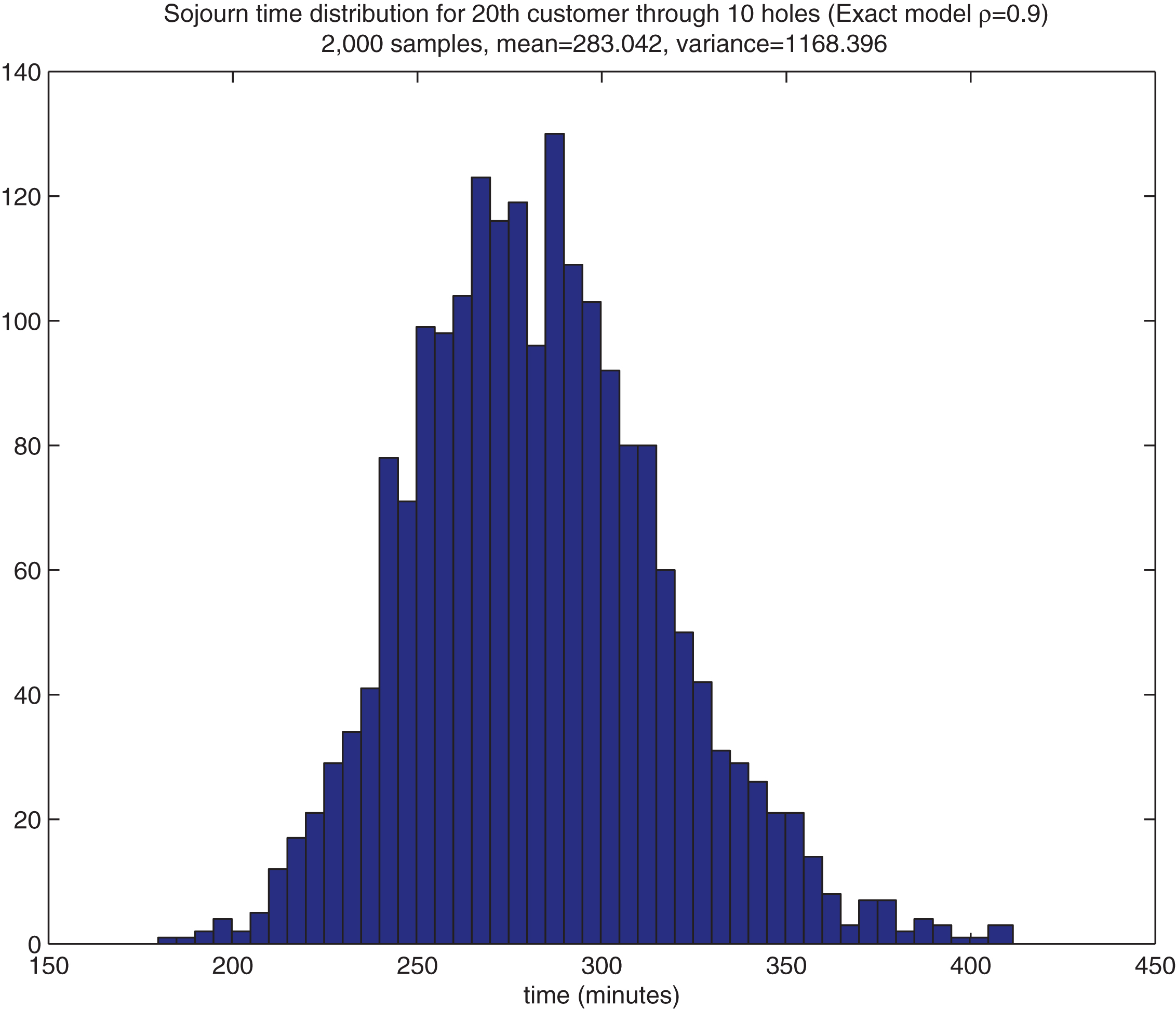
Fig.5
Histogram of the sojourn times V10,20 in the all exponential model with for ρ = 1.1.
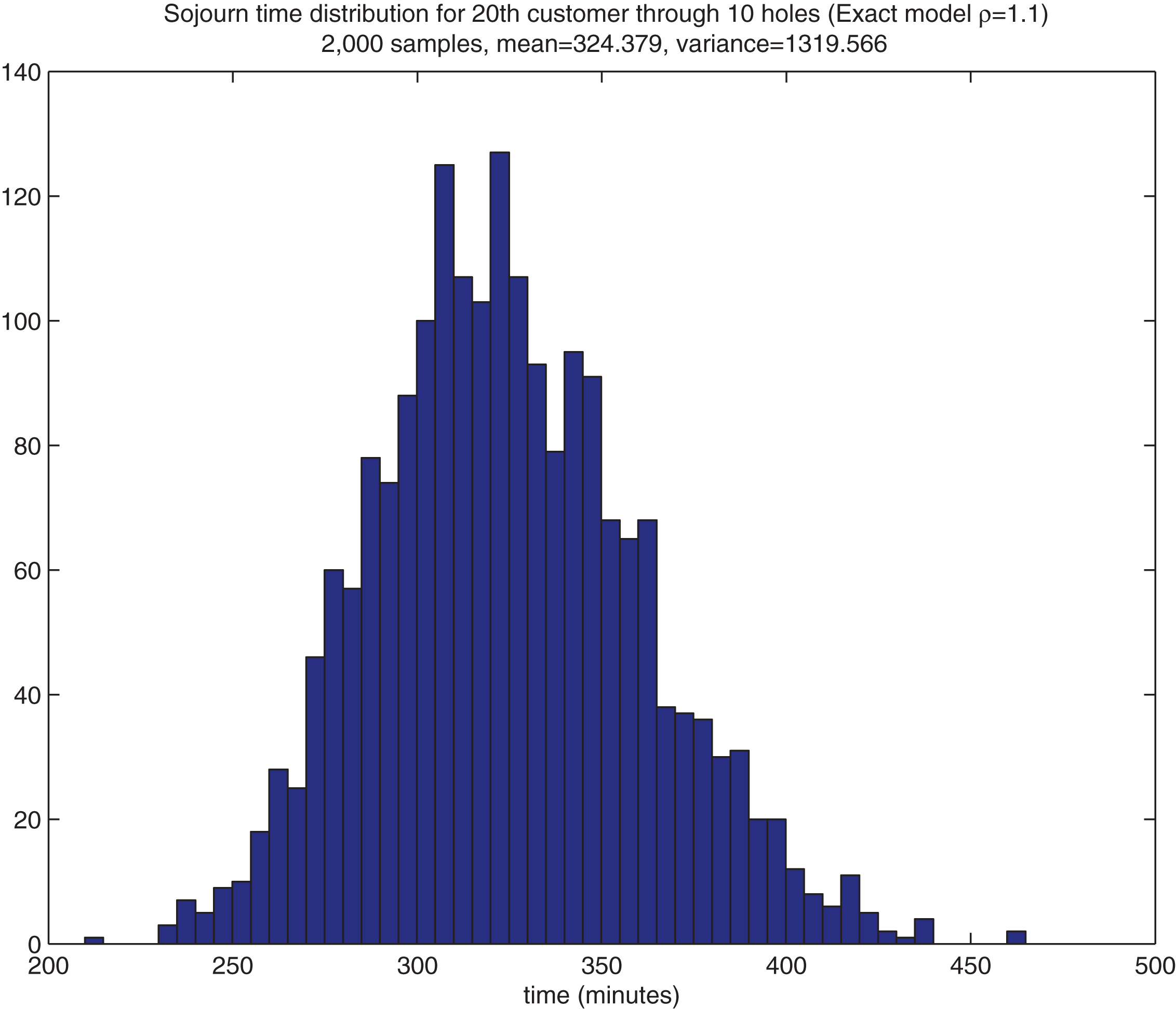
Table 1
Simulation comparison of the transient performance predicted by the exact and approximate models: estimates of the mean and standard deviation of the sojourn times of group 20 on several holes, (Uk,20), and over the first 10 holes, (V10,20), for a series of i.i.d. par-4 holes with exponential stage playing times, for three traffic intensities ρ = 0.9, 1.0 and 1.1
| traffic intensity perf. measure | ρ = 0.9 | ρ = 1.0 | ρ = 1.1 | |||
| mean | std dev | mean | std dev | mean | std dev | |
| hole 1, exact model | 28.0 | 18.1 | 36.6 | 22.3 | 48.4 | 26.5 |
| approx model | 30.6 | 20.3 | 38.9 | 23.1 | 52.6 | 27.9 |
| hole 2, exact model | 32.7 | 20.0 | 37.8 | 24.1 | 42.2 | 25.5 |
| approx model | 33.5 | 21.1 | 40.1 | 23.7 | 43.2 | 25.2 |
| hole 3, exact model | 31.1 | 20.4 | 34.8 | 21.7 | 35.6 | 22.5 |
| approx model | 33.9 | 21.7 | 36.9 | 22.6 | 38.1 | 23.7 |
| hole 6, exact model | 28.5 | 18.2 | 29.0 | 18.0 | 29.7 | 22.8 |
| approx model | 29.4 | 19.5 | 30.7 | 18.3 | 31.4 | 19.5 |
| hole 10, exact model | 25.1 | 16.1 | 26.0 | 16.8 | 25.8 | 16.8 |
| approx model | 27.1 | 17.5 | 27.7 | 16.6 | 27.9 | 16.6 |
| first 10 holes, exact model | 283.8 | 34.2 | 305.9 | 35.1 | 326.6 | 36.6 |
| approx model | 303.8 | 38.5 | 328.2 | 38.0 | 346.7 | 40.2 |
Table 2
Simulation comparison of the transient performance predicted by the exact and approximate models: estimates of the mean and standard deviation of the sojourn times of group 100 on several holes, (Uk,100), and over the full course of 18 holes, (V18,100), for a series of i.i.d. par-4 holes with traffic intensity ρ = 1.1 and three stage playing time distributions
| Distribution | tri.(m, a) = (6, 3) | tri. + LB (p, L) = (.05, 12) | expon. m = 6 | |||
| perf. measure | mean | std dev | mean | std dev | mean | std dev |
| hole 1, exact model | 103.6 | 15.8 | 106.4 | 19.0 | 142.7 | 66.1 |
| approx model | 108.4 | 15.9 | 111.1 | 19.3 | 144.8 | 65.9 |
| hole 2, exact model | 31.6 | 13.6 | 35.3 | 16.2 | 87.3 | 59.7 |
| approx model | 33.1 | 14.2 | 36.9 | 17.2 | 87.3 | 57.0 |
| hole 3, exact model | 26.4 | 10.3 | 29.6 | 12.7 | 65.7 | 46.3 |
| approx model | 27.7 | 10.6 | 30.4 | 13.2 | 68.3 | 47.1 |
| hole 6, exact model | 21.9 | 6.7 | 24.3 | 8.9 | 47.7 | 35.4 |
| approx model | 23.10 | 7.7 | 25.0 | 9.7 | 50.6 | 34.8 |
| hole 10, exact model | 20.4 | 5.8 | 21.8 | 7.0 | 40.7 | 30.1 |
| approx model | 21.7 | 6.8 | 23.0 | 8.2 | 41.3 | 27.9 |
| hole 18, exact model | 18.7 | 4.3 | 19.9 | 6.8 | 33.3 | 23.8 |
| approx model | 20.7 | 6.0 | 21.4 | 5.7 | 35.3 | 23.4 |
| first 18 holes, exact | 468.8 | 10.1 | 503.7 | 14.1 | 908.5 | 58.6 |
| approx model | 498.3 | 12.4 | 526.7 | 15.3 | 938.5 | 61.8 |
Table 3
Comparison with simulation estimates of the heavy-traffic approximation in (42) for the mean and
standard deviation of
| stage playing time dist. | exact (sim) | HT approx (42) | (41) | ||
| mean | SD | mean | SD |
| |
| ρ = 1.1 | |||||
| deterministic, m = 6 | 243 | 0.0 | 9.00 (27 + 0.00) =243 | 0.0 | 0.0000 |
| triangular, (m, a) = (6, 3) | 363 | 9.5 | 9.70 (27 + 11.75) =376 | 9.5 | 0.0253 |
| tri+LB, (p, L) = (.05, 12) | 398 | 14.0 | 9.97 (27 + 16.42) =433 | 11.6 | 0.0268 |
| exponential, m = 6 | 826 | 56.4 | 12.00 (27 + 44.1) =853 | 44.1 | 0.0517 |
| ρ = 1.0 | |||||
| deterministic, m = 6 | 162 | 0.0 | 9.00 (18 + 0.00) =162 | 0.0 | 0.0000 |
| triangular, (m, a) = (6, 3) | 278 | 9.5 | 9.70 (18 + 11.75) =289 | 7.3 | 0.0253 |
| tri+LB, (p, L) = (.05, 12) | 310 | 13.8 | 9.97 (18 + 16.42) =343 | 9.2 | 0.0268 |
| exponential, m = 6 | 722 | 56.7 | 12.00 (18 + 44.1) =749 | 38.7 | 0.0517 |
| ρ = 0.9 | |||||
| deterministic, m = 6 | 162 | 0.0 | 9.00 (18 + 0.00) =162 | 0.0 | |
| triangular, (m, a) = (6, 3) | 201 | 5.6 | 162 + 9.7 (18) (9) (0.0267) =204 | 7.3 | |
| tri+LB, (p, L) = (.05, 12) | 224 | 9.8 | 162 + 9.97 (18 (9) (0.0382) =224 | 9.2 | |
| exponential, m = 6 | 597 | 52.9 | 162 + 12 (18 (9) (0.375) (0.727) =691 | 38.7 | |
Table 4
Comparison of the heavy-traffic approximation for the mean sojourn time of group 100 on the full 18-hole golf course, E [V18,100], in (1) and (23) with simulation estimates for four different stage playing times for ρ = 0.9, 1.0 and 1.1
| stage playing time dist. | exact (sim) | model approx (sim) | HT approx (43) | |||
| mean | SD | mean | SD | mean | SD | |
| ρ = 1.1 | ||||||
| deterministic, m = 6 | 351 | 0.0 | 351 | 0.0 | 351 | 0.0 |
| triangular, (m, a) = (6, 3) | 469 | 10.1 | 498 | 12.4 | 484 | 12.2 |
| tri+LB, (p, L) = (.05, 12) | 503 | 14.2 | 526 | 15.3 | 531 | 14.2 |
| exponential, m = 6 | 908 | 61.7 | 938 | 61.0 | 961 | 50.0 |
| ρ = 1.0 | ||||||
| deterministic, m = 6 | 270 | 0.000 | 270 | 0.000 | 270 | 0.000 |
| triangular, (m, a) = (6, 3) | 382 | 9.9 | 411 | 12.7 | 396 | 10.0 |
| tri+LB, (p, L) = (.05, 12) | 416 | 14.4 | 437 | 15.3 | 440 | 11.8 |
| exponential, m = 6 | 807 | 59.0 | 832 | 60.5 | 852 | 44.1 |
| ρ = 0.9 | ||||||
| deterministic, m = 6 | 270 | 0.000 | 270 | 0.000 | 270 | 0.000 |
| triangular, (m, a) = (6, 3) | 306 | 6.6 | 312 | 8.8 | 312 | 7.9 |
| tri+LB, (p, L) = (.05, 12) | 330 | 11.9 | 335 | 11.9 | 332 | 8.9 |
| exponential, m = 6 | 683 | 56.2 | 707 | 60.6 | 852 | 44.0 |


