Simulation of spin-echo SANS (SESANS) using McStas on monochromatic and time of flight instruments

Parnell, Steven R.; Li, Fankang; Stevense, Wesley; Bouwman, Wim G.

doi:10.3233/JNR-240004

Simulation of spin-echo SANS (SESANS) using McStas on monochromatic and time of flight instruments

Article type: Research Article

Authors: Parnell, Steven R.^{a; *} | Li, Fankang^b | Stevense, Wesley^a | Bouwman, Wim G.^a

Affiliations: [a] Faculty of Applied Sciences, Delft University of Technology, Mekelweg 15, 2629 JB Delft, The Netherlands | [b] Neutron Technologies Division, Oak Ridge National Laboratory, Oak Ridge, 37831, USA

Correspondence: [*] Corresponding author. E-mail: s.r.parnell@tudelft.nl.

Keywords: Small angle scattering, Monte Carlo, spin echo, neutron, scattering

DOI: 10.3233/JNR-240004

Journal: Journal of Neutron Research, vol. Pre-press, no. Pre-press, pp. 1-12, 2024

Published: 16 April 2024

Get PDF

Abstract

We conduct simulations of Spin Echo Small Angle Neutron Scattering (SESANS) by employing Monte Carlo methods to a setup using four magnetic Wollaston prisms. Our primary focus involves the validation of these models, encompassing monochromatic scenarios across various neutron wavelengths to ascertain the reliability of the simulations. Subsequently, we extend this validation to encompass simulations in time-of-flight mode. Our model consistently and precisely predicts the scattering patterns emanating from dilute spheres in both monochromatic and time-of-flight modes. Notably, it also accurately reproduces the intricate encoding associated with scattering occurring between the third and fourth magnetic Wollaston prism, which provides us with another approach to increase the solid angle coverage of a SESANS instrument. This validation process conclusively demonstrates the efficacy of our simulation methods. Importantly, it paves the way for simulating more intricate and realistic instrumental configurations, broadening the horizons for future research endeavours.

1.Introduction

Since the invention of neutron scattering techniques, there has been a concerted endeavour to enhance the resolution. One avenue for achieving this objective involves exploiting the Larmor precession of neutron spins, whereby slight perturbations in neutron energy or momentum transfer induce notable variations in the Larmor phase [8]. This precession phenomenon is dictated by the magnetic field environment through which neutrons traverse. Diverse magnetic field configurations have been devised to encode a myriad of scattering geometries. However, a fundamental challenge arises from the inherent inhomogeneity in magnetic field distributions, potentially leading to aberrations in the accumulated Larmor phase during neutron traversal.

Recent advancements in finite element-based simulations for magnetic fields afford the opportunity to comprehensively assess and characterise magnetic field performance. Such evaluations facilitate the investigation and subsequent minimisation of aberrations in the Larmor phase of neutron spins, guided by specific criteria. Despite the progress in magnetic field simulations, a commensurate level of sophistication in modelling neutron instrumentation has been lacking – a gap that now beckons attention through simulation methodologies.

This study specifically focuses on the Spin Echo Small Angle Neutron Scattering (SESANS) technique, which utilises a series of inclined magnetic fields to encode scattering into neutron polarisation. For a comprehensive understanding, readers are directed to pertinent references [2,26,27].

With an increasing number of instruments adopting SESANS [3,6,14,22,24–26], there is burgeoning interest in employing Monte Carlo methods to optimise these instruments and associated techniques [4,19]. Until recently, accurate simulation of Larmor labelling for scattering from such instruments was unattainable. However, recent enhancements in scattering models for Small Angle Neutron Scattering (SANS) have rendered this achievable [5]. These advanced models not only predict the scattered beam but also effectively consider the transmitted direct beam. Given the expanding presence of spin echo instruments and routine application of the technique at time-of-flight sources, it becomes pivotal to validate instrument behaviour using detailed Monte Carlo models. SESANS is increasingly finding applications across diverse fields such as colloids [23,32], food science [2,31], composites [9], gravitational studies [7,21] and as a prospective quantum probe [16,30]. This study aims to contribute to these advancements by validating various components and simple setups against established theoretical frameworks.

In this work we utilise the McStas Monte Carlo Ray Tracing software [17,33–36]. The remainder of the structure of this paper is as follows. We first define the established analytical expressions which predict the expected SESANS correlation function and degree of scattering expected. We then test these in various stages in our simulations presented here. We also present a description and parameterisation of the components used in the simulations. The validation steps are as follows:

(1) Validate the sphere model against monochromatic SANS for different neutron wavelengths and both coherent and incoherent scattering.
(2) Validate the sphere model in time of flight (TOF), similar to (1), for both coherent and incoherent scattering.
(3) Validate the model for the Wollaston prism module by simulating this in monochromatic mode for several neutron wavelengths, considering simulations performed using the inclined foils [28].
(4) Combine the TOF setup with the Wollaston prism model to simulate TOF SESANS.
(5) Model a non-standard configuration with the sample between the third and fourth Wollaston prisms and compare against established theory.

Steps (1) and (2) are routine and included in Appendix B.1 for completeness.

2.Analytical correlation functions for dilute hard spheres

In any SESANS experiment, the measured quantity is the neutron polarisation as a function of the spin echo length. Typically, the polarisation resulting from scattering at the sample is normalised to the instrumental polarisation (PP0). This is measured as a function of length termed the spin-echo length δ, defined as follows:

(1)δ=cBLλ2cotθ

where c is a constant c=γmπh=1.476×1014T−1m−2, B is the strength of the magnetic field in the prisms, L is the separation between the prisms and θ is the angle between the hypotenuse of the prism and the beam direction as shown in Fig. 1.

Fig. 1.

Diagram illustrating a SESANS setup employing MWPs. The magnetic fields within the shaded and unshaded triangles are identical but antiparallel to each other. The solid black regions denote the π/2 flipper, with magnetic fields perpendicular to the MWPs. The path of the neutron beam is represented by the dashed line. This depiction is adapted from reference [22], with adjustments made to the axes to align with the coordinate system in McStas.

In SESANS the measured quantity of the polarisation can be expressed as;

(2)P(δ)=exp(Σt{G(δ)−1})

Here G(δ) is related to the Debye correlation function of the sample, for a dilute sphere sample with spheres of radius r, G(ζ) where ζ=δr is given analytically by [15];

(3)G(ζ)=ℜ{[1−(ζ2)]12(1+18ζ2)+12ζ2[1−(ζ4)2]ln[ζ2+(4−ζ2)12]}

Here ℜ denotes taking the real part, evaluated for δ in the range 0 → 2r. Σt is given by [1] as;

(4)Σt=32ϕ(1−ϕ)(Δρ)2λ2rd

Here d is the thickness of the sample and ϕ is the volume fraction. G(δ) is the correlation function and Σt a measure of the scattering power. For more details the reader is directed to references [1,23,32].

The form of G(δ) is depicted schematically in Fig. 2 (a) for two different sphere radii. The critical observation is that the correlation function approaches zero at the particle diameter. Figure 2 (b) illustrates the calculated polarisation for two monochromatic neutron wavelengths and a time-of-flight scan, highlighting the wavelength dependence on the scattering power. In Fig. 2 (c), the normalised scattering correlation function is presented, normalising out the neutron wavelength and sample thickness contributions. This results in a measured correlation function that is independent of the instrumental configurations and solely dependent upon the spin echo length and Σt.

Fig. 2.

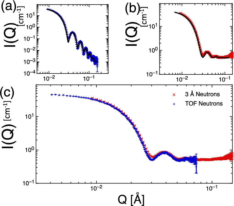
(a), the forms of G(δ) for dilute spheres are displayed as given by equation (3) for two different radii (as indicated in the legend). (b), the calculated polarisation as a function of spin echo length is depicted for two monochromatic neutron wavelengths and a time-of-flight scan. It’s important to note that in the time-of-flight simulation, we assume a static magnetic field of 117G, corresponding to a spin-echo length given by 15λ2 [Å²]. As a result, the TOF curve intersects the 3 Å curve at δ=1.8μ m and the 5 Å curve at 5 μm. Lastly, in (c), the three different simulations from (b) are corrected for wavelength, illustrating that they all converge onto the same curve, expressed as a normalised correlation function.

3.Components used

We now introduce the various components employed in this work and their associated parameterisation. SANS_spheres2 is a McStas component that mimics the scattering from a system of hard monodisperse dilute perfect spheres. An advantage of this sample over earlier samples defined for McStas is the consideration of both scattered and transmitted neutrons. Previous sample components only accounted for scattered neutrons, resulting in unrealistic SESANS outcomes. Further improvements include the distribution of scattered neutrons along a logarithmic distribution in the momentum transfer Q and the extension of the Q range to encompass the SESANS regime and the inclusion of multiple scattering [5,13].

The sample is initially utilised to simulate the expected scattering from a Small Angle Neutron Scattering (SANS) instrument, as shown in Appendix B.1. The sample configuration comprises a volume fraction ϕ of 0.001, a difference in scattering length density between the spheres and the solvent, denoted as Δρ, of 6·1010 cm−2, a radius r of 150 Å and a thickness of 1 mm. The outcomes of this simulation are detailed in Appendix B.1.

Neutrons possess the capability to scatter both coherently and incoherently from the sample. In the SANS_spheres2 sample, incoherent scattering is also considered, allowing the resultant simulation of an incoherent background, typical in more hydrogenous samples. Consequently, for dilute spheres, the scattering follows the conventional expression [10].

(5)I(Q)=ϕV(Δρ)2[3sin(Qr)−Qrcos(Qr)(Qr)3]2+Ibg

Here, V represents the volume of the sphere with radius r. A Q range from 1×10−5 Å⁻¹ to 0.4 Å⁻¹ and incoherent backgrounds of 0 and 0.5 cm⁻¹ are employed. To validate this sample component, simulations were conducted for regular monochromatic and TOF SANS setups, summarised in Section B.1. These simulations demonstrate that the component behaves as expected for two different incident neutron wavelengths in monochromatic mode and also in time of flight. Furthermore, it accurately accommodates the inclusion of incoherent scattering. The data obtained were fitted using SasView, resulting in derived radii and volume fractions that agree to within 0.1% with the input parameters, including the incoherent background when utilised.

For simulating a monochromatic neutron source, the source_simple component is utilised, representing a simple, rectangular neutron source targeting a rectangular target. The utilised source measures 6 cm × 6 cm, generating 1 × 10⁸ neutrons. Two neutron wavelengths of 3 Å and 5 Å are simulated to verify the wavelength dependence. 3 Å is short for a SANS instrument, however it is used here as SESANS instruments can often utilise short wavelength neutrons, for example in the Delft setup [28].

In the TOF setup, the source_gen component is used, allowing the specification of a range of wavelengths with a certain distribution. A wavelength range from 2 Å to 5 Å with a uniform distribution is employed, generating 1 × 10⁹ neutrons. This increased number of neutrons aims to ensure sufficient statistics due to the higher number of spin-echo length bins when scanning over a range of G(δ).

Two Monitor components in McStas are utilised, which return a simple count of neutrons. These monitors remain idealised and do not affect the passing neutrons. In the time-of-flight simulation, the monitors are replaced by the wavelength-sensitive monitor L_monitor in McStas, which counts the neutrons passing through, binned within the specified wavelength range. In both the monochromatic and TOF simulation these monitors are directly after the sample position in the direct beam.

For the final detector, a Position Sensitive Detector (PSD) of the PSD_monitor type is employed. This component consists of multiple pixels in both width and height, individually summing all neutrons passing through each pixel and outputting the total intensity for each pixel. The utilised PSD in the setup measures 1 m × 1 m and consists of 249 × 249 pixels. An example of a PSD measurement is depicted in Fig. 5 (b). In the time-of-flight setup, the PSD_TOF_monitor is used, binned within a specified time range.

Lastly, the setup includes source and sample apertures of the Slit component type in McStas. Circular apertures are employed with radii R1=5 mm and R2=5 mm for the source aperture and sample aperture, respectively.

4.Results of the SESANS simulation

The SESANS instrument in McStas is visualised in Fig. 9. Simulations were conducted for both the spin-up (I+) and spin-down (I−) configurations. This was achieved by altering the initial polarisation state and calculating P=(I+−I−)(I++I−). This could also be equally performed by adding in a flipper before the analyser, which would allow simulation of effects such as wavelength dependent flippers. In practical experiments, the measurement of empty beam polarisation is essential and the sample polarisation is usually corrected for this depolarisation. However, in this idealised scenario, such corrections are considered unnecessary as the empty beam polarisation is unity.

Starting with the monochromatic case, we conducted simulations where the magnetic field strength in the prisms was systematically varied to scan the spin-echo length (δ). The resulting polarisation is illustrated in Fig. 3 (a), showing good agreement with the anticipated theory discussed in Section 2. These simulations effectively capture both the expected shape of the correlation function G(δ) and the extent of depolarisation, which correlates with Σt – associated with the fraction of scattered neutrons within the transmitted beam [26]. Figure 3 (b) displays the successful representation of the two neutron wavelengths used, demonstrating consistent outcomes for 3 and 5 Å neutrons.

The time-of-flight simulation reproduces the green curve depicted in 3 (a), which is a fixed magnetic field with neutron wavelengths from 2–5 Å neutrons. When compared against the analytical function presented in 3 (b) (bottom green), a notable alignment is evident, signifying robust agreement. These straightforward simulations validate the efficacy of employing both the SANS_sphere2 scattering component and the Wollaston prism component. These results confirming our capability to accurately simulate instruments in both TOF and monochromatic modes.

Fig. 3.

In (a), the simulated polarisations for the two monochromatic neutron wavelengths, as indicated in the legend, are depicted alongside the results from the time-of-flight simulation. Meanwhile, (b) shows the normalised functions, accounting for wavelength and sample thickness effects. These corrected functions are compared with the calculated forms derived from equation (3). Note that the error bars are smaller than the points.

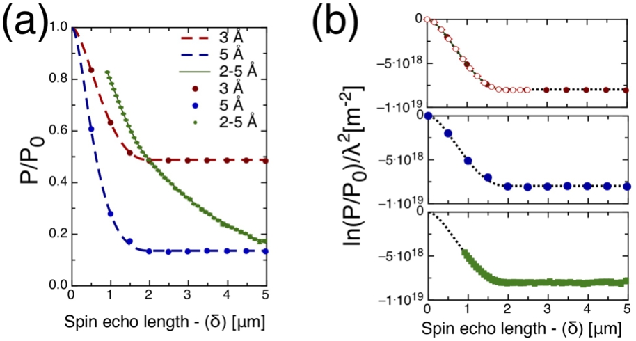
Fig. 4.

In (a), both the calculated and simulated normalised SESANS polarisations as a function of spin-echo length are depicted. The simulations are conducted with and without an incoherent background, as indicated in the legend, and also account for time-of-flight variations. Meanwhile, (b) demonstrates the corresponding alteration in the ‘apparent’ correlation length when the sample is positioned between magnets three and four. 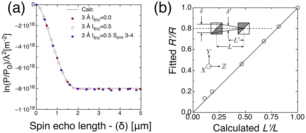The inset visualises the modified spin echo setup with the different sample position and shows how L′ is defined with respect to the sample and prisms. Note that the error bars are smaller than the points.

In most Small Angle Neutron Scattering (SANS) experiments, incoherent scattering often presents challenges by generating a high background, particularly at high Q values. However, SESANS is less significantly affected by such scattering. This is evident in the simulations presented in Fig. 4 (a), showcasing both monochromatic and time-of-flight simulations with and without incoherent scattering. Previous tests in a standard SANS configuration confirmed the presence of incoherent background scattering, showing reasonable agreement. However, the simulations consistently predict a slightly lower scattering intensity than the calculated values, a trend more pronounced in the time-of-flight case.

In the current Delft SESANS setups, detection of scattering from smaller structures (less than 100 nm), is difficult, due to the low magnetic fields required. Consequently, if the sample is positioned in a secondary location between the third and fourth encoding devices the accessible spin-echo length is reduced and given by;

(6)δ=cBL′λ2cotθ

Where L′ is the distance from the sample to the centre of the hypotenuse of prism four, as indicated in the inset of Fig. 4 (b). Typically this halves the spin echo length scale range. It is quite possible that this arrangement enhances the solid angle coverage, thereby extending the accessible Q range, albeit changing the spin echo length range, however this is a subject of further study [18] outside the scope of this article.

For a sample placed between prisms three and four, a spin echo length δ′ is defined for a given L′ (as shown in the inset of Fig. 4 (b)). Consequently, as the angle ϑ remains constant, δ′δ=L′L. Therefore, we anticipate the probed spin echo length range to be altered from the traditional sample position by a factor of L′L. SESANS was implemented in this configuration, and the resulting correlation function was fitted. It’s important to note that the spin-echo length (δ) is calculated using equation (6), and the ratio of the determined radius (R′) over the model radius (R) is plotted in Fig. 4 (b) for various sample positions. This representation demonstrates good agreement between the calculated and simulated values.

5.Discussion and future directions

The comprehensive simulations conducted in this study elucidate various aspects of SESANS setups, affirming the efficacy of McStas in modeling this technique. This research complements prior demonstrations of monochromatic SESANS and SEMSANS [5]. Moreover, recent advancements have highlighted McStas’ capacity to model intricate setups involving a sequence of MWPs [20].

While certain sample characteristics such as absorption and multiple scattering are presently absent, their inclusion would be beneficial. Recent studies investigating multiple scattering effects suggest the feasibility of incorporating these phenomena into the model [13].

It’s important to note that our approach is purely classical, accounting only for the net Larmor phase accumulated by the neutron as it traverses through the instrument. Although quantum descriptions of polarized neutron state interactions are possible [12,16,30], these aspects are not replicated in this Monte Carlo model.

Another significant avenue involves integrating SEMSANS with SANS [29], which offers a comprehensive understanding of hierarchical structures. A straightforward strategy could entail stacking two samples of spheres with different sizes, facilitating simultaneous simulation of scattering at two distinct length scales. This presents an opportunity for more detailed optimization of instrument geometry, focusing on angular acceptance, and potentially yielding a more refined treatment of data compared to our current phenomenological method of transmission corrections [18].

6.Conclusions

This study successfully validates SESANS simulations across various neutron wavelengths and, notably, for the first time in a TOF setup. These simulations provide a framework for extracting SESANS results, allowing exploration of changes in sample positioning and incorporation of incoherent scattering effects. The anticipated outcome is the utilization of these tools to enhance the precision of the techniques and foster the development of novel and advanced instrumental setups.

Acknowledgements

We acknowledge the valuable discussions with the McStas team. Special thanks to Mads Bertelsen for his assistance with the McStas script interface, installation, and general support. Additionally, we appreciate the contributions of Jasmijn van Arnhem from TU Delft for guiding the direction of this project.

This work is supported by the US Department of Energy (DOE), Office of Science, Office of Basic Energy Sciences, Early Career Research Program Award (KC0402010) with proposal No. (ERKCSA4), under Contract No. DE-AC05-00OR22725.

7.Declaration

This manuscript has been authored by UT-Battelle, LLC under Contract No. DE-AC05-00OR22725 with the U.S. Department of Energy. The United States Government retains and the publisher, by accepting the article for publication, acknowledges that the United States Government retains a non-exclusive, paid-up, irrevocable, world-wide license to publish or reproduce the published form of this manuscript, or allow others to do so, for United States Government purposes. The Department of Energy will provide public access to these results of federally sponsored research in accordance with the DOE Public Access Plan (http://energy.gov/downloads/doe-public-access-plan).

Appendices

Appendix A.

Appendix A.Guide for the data reduction and simulation Python code

All of the simulations are done using McStasScript https://github.com/PaNOSC-ViNYL/McStasScript. This is a Python scripting language that can be used to automate McStas simulations. The full Python code containing the developed data reduction method and a script for all the simulations done can be found here http://github.com/WesleyStevense/SANS_spheres2_model. This appendix serves as a quick guide through the most important parts of the code.

The Wollaston_prism component is also included which is used for the prisms. A more advanced version which allows for variable hypotenuse angle is in preparation and will be sent to the McStas team.

Monochromatic SANS. Monochromatic SANS simulations can be done using the monochromatic class. All relevant simulation parameters can be set when initialising the class. When the class is initialised, the monochromatic_model is called to run the simulation. The monochromatic_model class has the method scatterplot() that creates a scatterplot of the PSD measurement. Furthermore the absolute_calibration() method does the 2D data calibration. Finally the intensity_plot() method does the full data reduction. The function get_q_profile() is called to do the radial averaging and the binning() function is used to do the binning.

TOF SANS. TOF SANS simulations can be done using the TOF class. Allrelevant simulation parameters can be set when initialising the class. When the class is initialised, the TOF_model is called to run the simulation. The TOF class has the method intensity_plot_q(index) to do the full data reduction on each PSD bin, again calling the get_q_profile function to do this. An index has to be passed to this method to tell it which PSD bin index to take. Furthermore the intensity_plot() method that calls the intensity_plot_q(index) for each PSD snapshot and bins them using the binning() function, yielding the final result.

Monochromatic SESANS. Monochromatic SESANS simulations can be done using the SESANS class. All relevant simulation parameters can be set when initialising the class. When the class is initialised, the SESANS_model is called to run the simulation. The SESANS class has the method plot_I to plot the I+ and I− results. The spin_echo_length() method is used to calculate the probed spin echo length δ), and finally the plot_pol_lambda() method can be used to plot the final result.

TOF SESANS. Monochromatic SESANS simulations can be done using the TOF_SESANS class. All relevant simulation parameters can be set when initialising the class. When the class is initialised, the TOF_SESANS_model is called to run the simulation. The SESANS class has the method spin_echo_length() to calculate all the probed spin echo length (δ) and finally the plot_pol_lambda() method can be used to plot the final result.

Appendix B.

Appendix B.SANS modelling

B.1.SANS – monochromatic

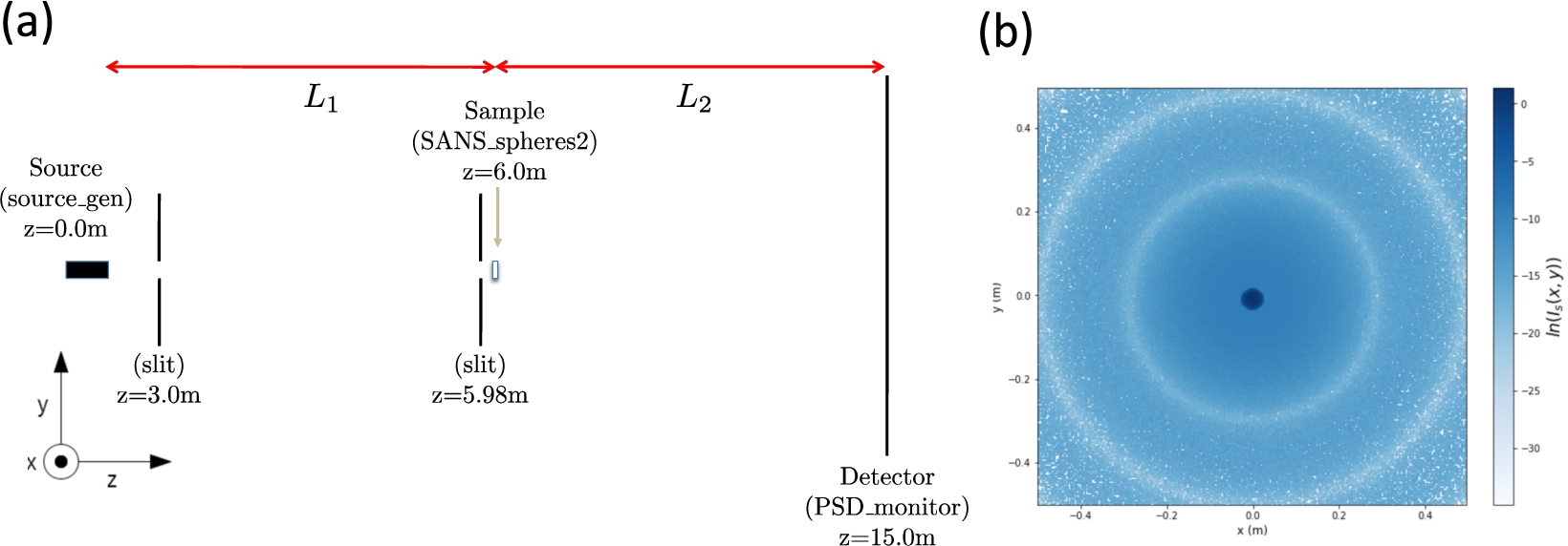
To test the spheres component we use a the monochromatic SANS setup shown in Fig. 5 (a). Corrections are done on the 2D PSD data following established procedures [11] to correct for solid angle and the planar geometry. It is then correction for the sample transmission T. T is retrieved from the output data as I1I0. Finally the data also has to be corrected for the sample thickness and empty beam transmission yielding the final corrected data dΣdΩ(x,y) to be [11]

(7)dΣ(x,y)dΩ=Is(x,y)I0TdΔΩ.

As SANS data is then converted to Q and placed in radially symmetric bins, as the scattering is isotropic.

Fig. 5.

Shown in (a) is a schematic representation of the setup used in the simulation of the monochromatic SANS instrument, specifying all used McStas components in brackets and location (z) in metres. Drawing is not to scale. In (b) is the 2-D PSD_monitor component output, plotted in the 2D plane for all pixels, showing a clear ring pattern, as expected for scattering from isotropic monodisperse spheres.

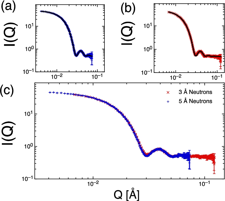
The results of the two monochromatic SANS simulations are shown in Fig. 6, where we also added an incoherent component background. The data was fitted in SASView and values for the dilute spheres were within 0.1% of the McStas sphere component values which we deem as good agreement. It should be noted that the small increase in resolution is expected following from the use of longer wavelength neutrons.

Fig. 6.

Shown are simulations for the scattering from monodisperse spheres (with incoherent background Ibg=0.5 cm−1) on a monochromatic SANS instrument at 3 and 5 Å. In (a). and (b) is the simulated data along with a fit using the sphere parameters specified in Section 3 for 5 Å (a) and 3 Å (b) neutrons. Shown below (c) is the overlapped data for both wavelengths again showing good agreement between both simulations, except as expected a small change in resolution.

B.2.SANS – time of flight (TOF)

The time of flight setup is of course similar to the monochromatic setup. The source with a uniform wavelength distribution is placed at the origin. As in the monochromatic case, the sample will again be at a distance L1 of 6 m away in the z direction from the source. Again, at 3 m from the source, the source aperture will be placed and at 2 mm before the sample the sample aperture will be placed. At 1 mm before the sample and 1 mm after the sample the idealised wavelength dependent monitors will be placed. The output of the monitor before the sample is the empty beam transmission and will now be wavelength dependent and be denoted by I0(λ). The output of the monitor after the sample will be denoted by I1(λ). Then at a distance of L2 of 9 m away from the source, the time of flight PSD will be placed. The output of the PSD will now be dependent of time and be denoted by Is(x,y,t). A schematic representation of the setup is shown in Fig. 7. As the output of the PSD is in time and everything will be analysed in wavelength, time has to be converted to wavelength allowing us to convert Is(x,y,t) to Is(x,y,λ).

Fig. 7.

Schematic representation of the setup used in the simulation of the TOF SANS instrument, specifying all used McStas components. Drawing is not to scale.

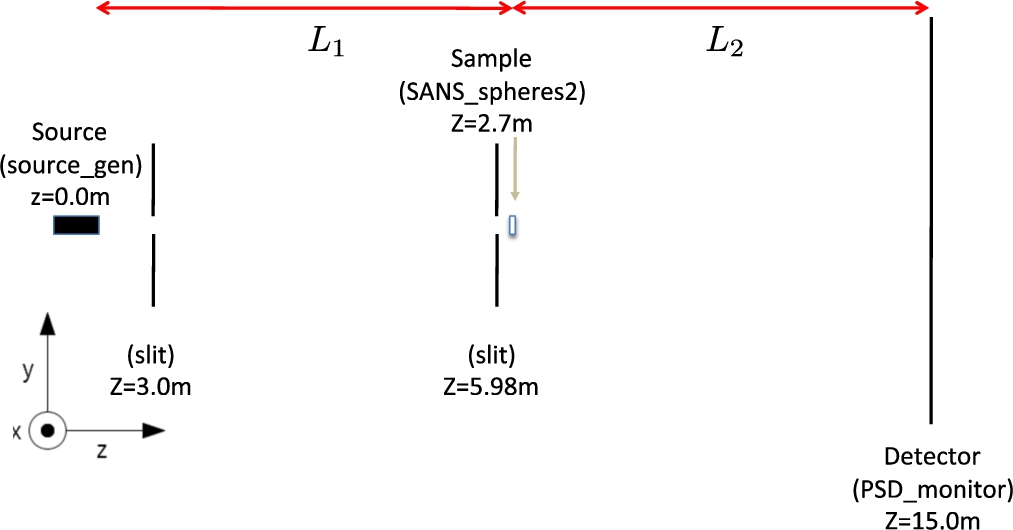
Fig. 8.

Shown are simulations for the scattering (in time of flight) from monodisperse spheres for pure coherent scattering (a) and with incoherent background Ibg=0.5 cm−1 (b). In (a) and (b) is the simulated data along with a fit using the sphere parameters specified in Section 3 for 5 Å (a) and 3 Å (b) neutrons. Shown below (c) is the overlapped data for both monochromatic and using 5 Å neutrons and TOF again showing good agreement between both simulations.

As the positions of the two monitors and the position of the PSD are far apart, it is possible that the binned wavelengths wavelength dependent monitors do not exactly match those of the calculated ones at the PSD position. This means the values of I0(λ) and I1(λ) have to be linearly interpolated to obtain values over the whole wavelength range. Using these interpolated values, T(λ) (over the whole wavelength range) can be obtained as I1(λ)I0(λ). The corrected TOF data is again radially averaged. The same procedure as in the monochromatic case be applied to each PSD snapshot. The radially averaged data now has to be binned in similar way to the monochromatic data for a given neutron wavelength and then all wavelengths converted to Q to yield the resulting SANS dataset as shown in Fig. 8.

For the time of flight SANS setup the data were again analysed using SASView, the fitted parameters were indeed within error identical to those proscribed in the sample model. Thus confirming the effectiveness of the model in standard SANS TOF geometry.

Appendix C.

Appendix C.SESANS component layout

For the SESANS work, the precise geometry used in these simulations along with the McStas components used is shown in Fig. 9.

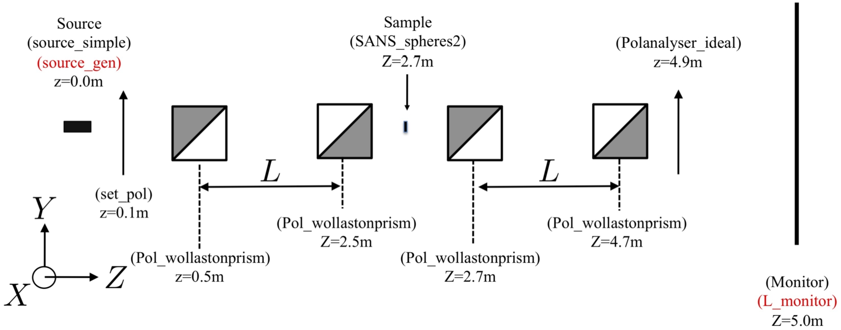
Fig. 9.

Visual depiction of the SESANS instrument simulation setup, detailing the employed McStas components. The illustration is not drawn to scale. Components represented in black correspond to the monochromatic setup, while those in red signify alterations made for the TOF simulations. Note that the sample is 2 mm in front of the third prism.

References

[1]	R. Andersson, L.F. Van Heijkamp, I.M. De Schepper and W.G. Bouwman, Analysis of spin-echo small-angle neutron scattering measurements, Journal of Applied Crystallography 41: (5) ((2008) ), 868–885. doi:10.1107/S0021889808026770.
[2]	W.G. Bouwman, Spin-echo small-angle neutron scattering for multiscale structure analysis of food materials, Food Structure 30: ((2021) ), 100235. ISBN 2213-3291. doi:10.1016/j.foostr.2021.100235. https://www.sciencedirect.com/science/article/pii/S2213329121000587.
[3]	W.G. Bouwman, C.P. Duif and R. Gähler, Spatial modulation of a neutron beam by Larmor precession, Physica B: Condensed Matter 404: (17) ((2009) ), 2585–2589. doi:10.1016/j.physb.2009.06.052.
[4]	W.G. Bouwman, C.P. Duif, J. Plomp, A. Wiedenmann and R. Gähler, Combined SANS–SESANS, from 1 nm to 0.1 mm in one instrument, Physica B: Condensed Matter 406: (12) ((2011) ), 2357–2360. doi:10.1016/j.physb.2010.11.069.
[5]	W.G. Bouwman, E.B. Knudsen, L. Udby and P. Willendrup, Simulations of foil-based spin-echo (modulated) small-angle neutron scattering with a sample using McStas, Journal of Applied Crystallography 54: (1) ((2021) ), 195–202. https://doi.org/10.1107/S1600576720015496. doi:10.1107/S1600576720015496.
[6]	R. Dadisman, J. Shen, H. Feng, L. Crow, C. Jiang, T. Wang, Y. Zhang, H. Bilheux, S.R. Parnell, R. Pynn and F. Li, Design and characterization of zero magnetic field chambers for high efficiency neutron polarization transport, Nuclear Instruments and Methods in Physics Research Section A: Accelerators, Spectrometers, Detectors and Associated Equipment 940: ((2019) ), 174–180. doi:10.1016/j.nima.2019.05.092.
[7]	V.-O. de Haan, J. Plomp, A.A. van Well, M.T. Rekveldt, Y.H. Hasegawa, R.M. Dalgliesh and N.-J. Steinke, Measurement of gravitation-induced quantum interference for neutrons in a spin-echo spectrometer, Phys. Rev. A 89: ((2014) ), 063611. doi:10.1103/PhysRevA.89.063611.
[8]	B. Farago, Neutron Spin Echo Spectroscopy: Basics, Trends and Applications, Lecture Notes in Physics, Springer, Berlin, Heidelberg, (2003) .
[9]	H. Gaspar, P. Teixeira, R. Santos, L. Fernandes, L. Hilliou, M.P. Weir, A.J. Parnell, K.J. Abrams, C.J. Hill, W.G. Bouwman, S.R. Parnell, S.M. King, N. Clarke, J. Covas and G. Bernardo, A journey along the extruder with polystyrene:C60 nanocomposites: Convergence of feeding formulations into a similar nanomorphology, Macromolecules 50: (8) ((2017) ), 3301–3312. doi:10.1021/acs.macromol.6b02283.
[10]	A. Guinier and G. Fournet, Small Angle Scattering of X-rays, Wiley and Sons and Chapman and Hall Ltd., (1955) .
[11]	B. Hammouda, Probing Nanoscale Structures – the SANS Toolbox, National Institute of Standards and Technology Center for Neutron Research Gaithersburg, (2008) .
[12]	A.A.M. Irfan, P. Blackstone, R. Pynn and G. Ortiz, Quantum entangled-probe scattering theory, 23: (8) ((2021) ), 083022. ISBN 1367-2630. doi:10.1088/1367-2630/ac12e0. https://dx.doi.org/10.1088/1367-2630/ac12e0.
[13]	S. Jaksch, V. Pipich and H. Frielinghaus, Multiple scattering and resolution effects in small-angle neutron scattering experiments calculated and corrected by the software package MuScatt, Journal of Applied Crystallography 54: (6) ((2021) ), 1580–1593. doi:10.1107/S1600576721009067.
[14]	T. Keller, R. Gähler, H. Kunze and R. Golub, Features and performance of an NRSE spectrometer at BENSC, Neutron News 6: (3) ((1995) ), 16–17. doi:10.1080/10448639508217694.
[15]	T. Krouglov, W.G. Bouwman, J. Plomp, M.T. Rekveldt, G.J. Vroege, A.V. Petukhov and D.M.E. Thies-Weesie, Structural transitions of hard-sphere colloids studied by spin-echo small-angle neutron scattering, Journal of Applied Crystallography 36: (6) ((2003) ), 1417–1423. doi:10.1107/S0021889803021216.
[16]	S.J. Kuhn, S. McKay, J. Shen, N. Geerits, R.M. Dalgliesh, E. Dees, A.A.M. Irfan, F. Li, S. Lu, V. Vangelista, D.V. Baxter, G. Ortiz, S.R. Parnell, W.M. Snow and R. Pynn, Neutron-state entanglement with overlapping paths, Phys. Rev. Res. 3: ((2021) ), 023227. doi:10.1103/PhysRevResearch.3.023227.
[17]	K. Lefmann and K. Nielsen, McStas, a general software package for neutron ray-tracing simulations, Neutron News 10: (3) ((1999) ), 20–23. https://doi.org/10.1080/10448639908233684. doi:10.1080/10448639908233684.
[18]	F. Li, S.R. Parnell, R. Dalgliesh, A. Washington, J. Plomp and R. Pynn, Data correction of intensity modulated small angle scattering, Scientific Reports 9: (1) ((2019) ), 8563. doi:10.1038/s41598-019-44493-9.
[19]	F. Li, S.R. Parnell, W.A. Hamilton, B.B. Maranville, T. Wang, R. Semerad, D.V. Baxter, J.T. Cremer and R. Pynn, Superconducting magnetic Wollaston prism for neutron spin encoding, Review of Scientific Instruments 85: (5) ((2014) ). doi:10.1063/1.4878715.
[20]	S.R. Parnell, S.V.D. Berg, G. Bolderink and W.G. Bouwman, Simulations and concepts for a 2-D spin-echo modulated SANS (SEMSANS) instrument, Journal of Physics: Conference Series 2481: (1) ((2023) ), 012007. doi:10.1088/1742-6596/2481/1/012007.
[21]	S.R. Parnell, A.A. van Well, J. Plomp, R.M. Dalgliesh, N.-J. Steinke, J.F.K. Cooper, N. Geerits, K.E. Steffen, W.M. Snow and V.O. de Haan, Search for exotic spin-dependent couplings of the neutron with matter using spin-echo based neutron interferometry, Phys. Rev. D 101: ((2020) ), 122002. doi:10.1103/PhysRevD.101.122002.
[22]	S.R. Parnell, A.L. Washington, K. Li, H. Yan, P. Stonaha, F. Li, T. Wang, A. Walsh, W.C. Chen, A.J. Parnell, J.P.A. Fairclough, D.V. Baxter, W.M. Snow and R. Pynn, Spin echo small angle neutron scattering using a continuously pumped 3He neutron polarisation analyser, Review of Scientific Instruments 86: (2) ((2015) ), 023902. doi:10.1063/1.4909544.
[23]	S.R. Parnell, A.L. Washington, A.J. Parnell, A. Walsh, R.M. Dalgliesh, F. Li, W.A. Hamilton, S. Prevost, J.P.A. Fairclough and R. Pynn, Porosity of silica Stober particles determined by spin-echo small angle neutron scattering, Soft Matter 12: ((2016) ), 4709–4714. doi:10.1039/C5SM02772A.
[24]	J. Plomp, V.O. de Haan, R.M. Dalgliesh, S. Langridge and A.A. van Well, Neutron spin-echo labelling at OffSpec, an ISIS second target station project, Thin Solid Films 515: (14) ((2007) ), 5732–5735. doi:10.1016/j.tsf.2006.12.129.
[25]	R. Pynn, Neutron Spin Echo, F. Mezei, ed., Lecture Notes in Physics, Vol. 128: , Springer, Heidelberg, (1980) , pp. 159–177. doi:10.1007/3-540-10004-0_29.
[26]	M.T. Rekveldt, Novel SANS instrument using Neutron Spin Echo, Nuclear Instruments and Methods in Physics Research Section B: Beam Interactions with Materials and Atoms 114: (3–4) ((1996) ), 366–370.
[27]	M.T. Rekveldt, Neutron reflectometry and SANS by neutron spin echo, Physica B: Condensed Matter 234–236: (0) ((1997) ), 1135–1137. doi:10.1016/S0921-4526(97)00138-5.
[28]	M.T. Rekveldt, J. Plomp, W.G. Bouwman, W.H. Kraan, S. Grigoriev and M. Blaauw, Spin-echo small angle neutron scattering in Delft, Review of Scientific Instruments 76: (3) ((2005) ), 033901. doi:10.1063/1.1858579.
[29]	J. Schmitt, J.J. Zeeuw, J. Plomp, W.G. Bouwman, A.L. Washington, R.M. Dalgliesh, C.P. Duif, M.A. Thijs, F. Li, R. Pynn, S.R. Parnell and K.J. Edler, Mesoporous silica formation mechanisms probed using combined spin–echo modulated small-angle neutron scattering (SEMSANS) and small-angle neutron scattering (SANS), ACS Applied Materials & Interfaces 12: (25) ((2020) ), 28461–28473. doi:10.1021/acsami.0c03287.
[30]	J. Shen, S.J. Kuhn, R.M. Dalgliesh, V.O. de Haan, N. Geerits, A.A.M. Irfan, F. Li, S. Lu, S.R. Parnell, J. Plomp, A.A. van Well, A. Washington, D.V. Baxter, G. Ortiz, W.M. Snow and R. Pynn, Unveiling contextual realities by microscopically entangling a neutron, Nature Communications 11: (1) ((2020) ), 930. doi:10.1038/s41467-020-14741-y.
[31]	B. Tian, Z. Wang, A.J. van der Goot and W.G. Bouwman, Air bubbles in fibrous caseinate gels investigated by neutron refraction, X-ray tomography and refractive microscope, Food Hydrocolloids 83: ((2018) ), 287–295. doi:10.1016/j.foodhyd.2018.05.006.
[32]	A.L. Washington, X. Li, A.B. Schofield, K. Hong, M.R. Fitzsimmons, R. Dalgliesh and R. Pynn, Inter-particle correlations in a hard-sphere colloidal suspension with polymer additives investigated by Spin Echo Small Angle Neutron Scattering (SESANS), Soft Matter 10: ((2014) ), 3016–3026. doi:10.1039/C3SM53027B.
[33]	P. Willendrup, E. Farhi, E. Knudsen, U. Filges and K. Lefmann, McStas: Past, present and future 17: ((2014) ), 35–43. doi:10.3233/JNR-130004.
[34]	P. Willendrup, E. Farhi and K. Lefmann, McStas 1.7 – a new version of the flexible Monte Carlo neutron scattering package, Physica B: Condensed Matter 350: (1, Supplement) ((2004) ), 735–737. Proceedings of the Third European Conference on Neutron Scattering, ISSN 0921-4526. https://www.sciencedirect.com/science/article/pii/S0921452604004144. doi:10.1016/j.physb.2004.03.193.
[35]	P.K. Willendrup and K. Lefmann, McStas (i): Introduction, use, and basic principles for ray-tracing simulations, 22: ((2020) ), 1–16. ISBN 1477-2655. doi:10.3233/JNR-190108.
[36]	P.K. Willendrup and K. Lefmann, McStas (ii): An overview of components, their use, and advice for user contributions, 23: ((2021) ), 7–27. ISBN 1477-2655. doi:10.3233/JNR-200186.