
Coupling NMR to SANS: Addressing at once structure and dynamics in soft matter
Abstract
In soft condensed matter, Small Angle Neutron Scattering (SANS) is a central tool to probe structures with characteristic sizes ranging from 1 to 100 nm. However, when used as a standalone technique, the dynamic properties of the sample are not accessible. Nuclear Magnetic Resonance (NMR) is a versatile technique which can easily probe dynamical information. Here, we report on the coupling of a low-field NMR system to a SANS instrument. We show that this original set-up makes it possible to obtain structural information and to simultaneously extract in situ on a same sample, long-range translational diffusion coefficient,
1.Introduction
Gels are macromolecular networks. Describing their structure and physical properties comes to understand the processes leading to their formation. Gelation is the result of a mechanism where individual molecules (monomers or polymer chains) are able to bind to at least three of their neighbors. The population of the remaining free molecules is soluble (hence the term of sol) until the appearance of a structure of infinite size: the gel. From a fundamental point of view, gelation is not a thermodynamic transition, but instead a critical transition of connectivity. Regardless of the local rules governing this connectivity, the machinery of critical phenomena can be used to describe all physical, chemical or biological processes where association of elementary molecules, initially separated from each other, leads to the formation of large clusters, then to macroscopic phases. The measurable static and/or dynamic quantities diverge at the gelation threshold and follow a power law behavior when they are expressed as a function of the gap to this point [1,2].
Catching simultaneously sharply evolving dynamical and structural quantities demands experimental techniques able to monitor the spatial dependence of correlation times. Light [3] and neutron scattering, in particular Neutron Spin-Echo (NSE) [4], have indeed shown large success in the field. But, despite the scientific need, the possibility to reach the 0.1 to
In this paper we report the first, to our knowledge, coupling of NMR and SANS and address the temperature-induced phase separation of a concentrated Poly(Methacrylic Acid) (PMAA, [–CH2–C–COOH–CH 3–]n) solution at its Lower Critical Solution Temperature (LCST). The driving force of such transitions is usually the entropy gain associated to the release of the solvent: as the water molecules experience a reduced number of hydrogen bonds with the polymer chains, their entropy increases. The conformation of this polyelectrolyte is driven by both the intra- and inter-chain competitions of i) intermolecular hydrogen bonds between carboxyl groups, and ii) hydrophobic interactions induced by the presence of methyl side-chains. It may be tuned by the pH and/or ionic strength. At low pH when PMAA stands in its acidic form (degree of ionization
Up to date, this temperature-induced phase separation of PMAA has been poorly addressed in the literature. It has been proposed that the gelation process could be induced by physical cross-linking of neighboring chains. If this is the case, one expects that the structuration of the gel has a strong influence on the behavior of the sol phase (the solvent). In this work, the characteristic sizes related to the domain growth of the polymer-rich phase are monitored by the evolution of the SANS spectra while the dynamics of the protonated moieties of the system (H2O and polymer) are simultaneously characterized (
2.Materials and methods
2.1.Sample
To minimize the incoherent background and to optimize the coherent contrast between polymer and solvent, SANS experiments on aqueous polymer solutions are usually performed using D2O. In the present framework of NMR/SANS coupling, to maximize the NMR sensitivity, the NMR radiofrequency of the probe was set on the resonance of the
PMAA (fully hydrogenated) was purchased from Polymer Science Inc. Its molar mass and molar mass distribution were obtained using Size Exclusion Chromatography (SEC). Prior to analysis, the polymer was modified by methylation of the carboxylic acid group using trimethylsilyldiazomethane. The samples were analyzed in tetrahydrofuran (THF) at a concentration of 10 mg/ml at 25°C. The column used was a polystyrene mixed C13 column for organic solvents. The setup was equipped with a refractive index (
2.2.SANS instrumental settings
In order to ensure the exact same experimental conditions for both the SANS and the NMR measurements, a home-made single-sided NMR spectrometer (see details in Section 3) was installed on the PAXY instrument [12] of the LLB (Laboratoire Léon Brillouin, Saclay, France). The SANS incident wavelength and sample to detector distances were,
3.NMR set-up
3.1.A home-made portable single-sided NMR setup
Many single sided NMR systems have been proposed in the literature [13]. Our approach to magnet design is based on the Spherical Harmonic Decomposition methodology to lead to a 12-fold cylindrically symmetric one-sided constant-gradient magnet without pole pieces [14,15], which has been used already to measure one-dimensional proton density profiles as well as relaxations and diffusions [16,17]. Our permanent magnet is a cylinder of 24 cm in diameter, 22 cm in height containing NdFeB magnets and weights ∼ 40 kg.
Its design consist in a simple dipole pointing along the z direction in the laboratory frame [14,15]. To ease its construction, we assembled and glued all magnet pieces non-magnetized and we magnetized it afterwards in a one-step process using a powerful electromagnet at the LNCMI-CNRS facility [14].
This device produces a magnetic field strength of
A single channel Tecmag’s Scout spectrometer and a Tomco© BT01000-Gamma power amplifier were used. The radio-frequency probe consisted of a rectangular shape copper coil with 10 turns tightly wound to fit a 1 mm thick Hellma® quartz cuvette, with total length 50 mm, and an external box in which the parallel and series mounted capacitors to the coil were accommodated, for the tuning and matching of the probe.
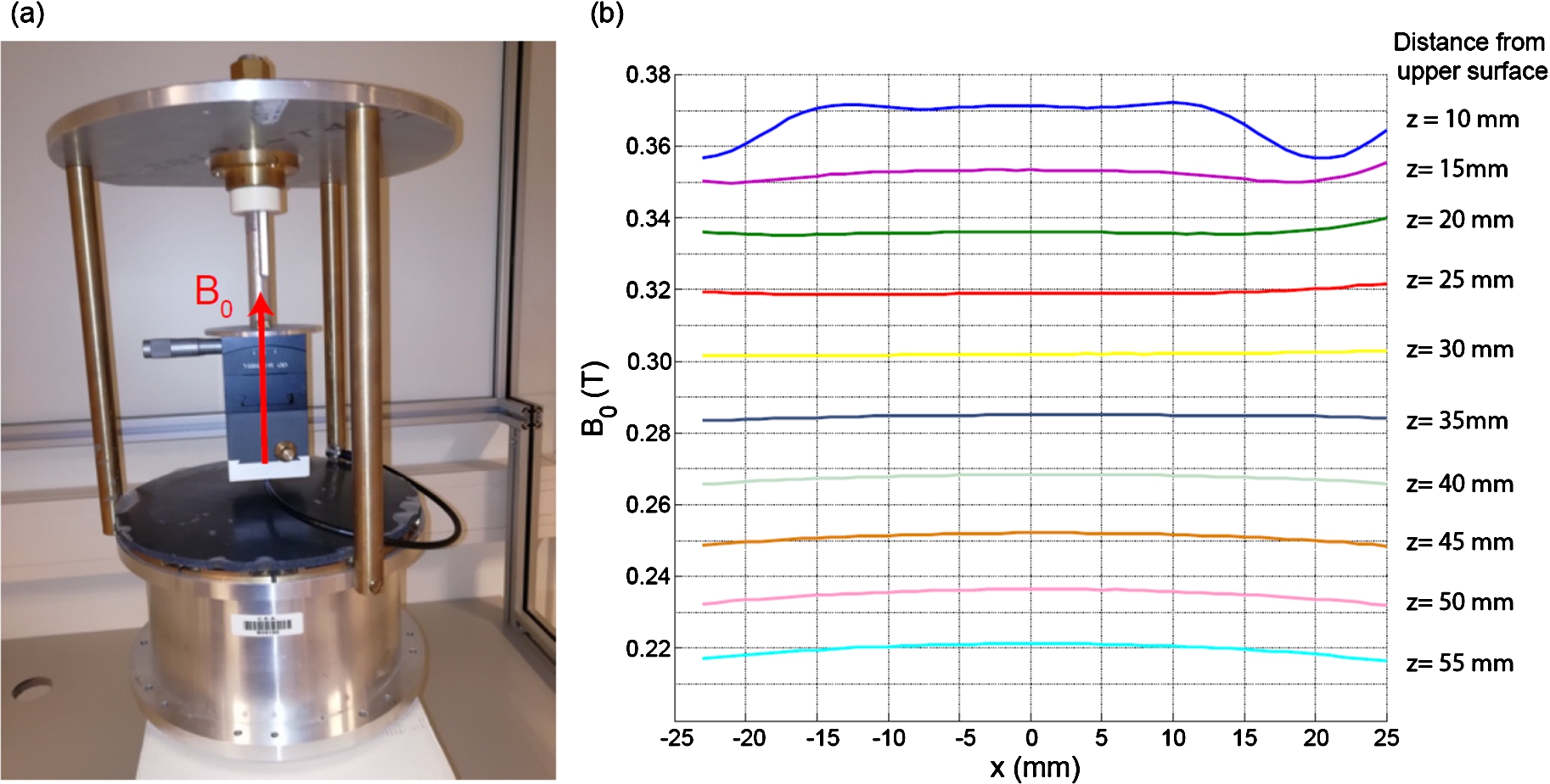
Fig. 1.
(a) Setup of NMR magnet and probe: the cylindrical NdFeB magnet assembly sits on an aluminum table and the goniometric probe is located along the central axis above the magnet. The sample is fixed inside the coil of the probe, which is precisely positioned by two non-magnetic goniometric stages fixed perpendicular to each other. The vertical position of the probe is controlled by a central threaded rod, which is fixed on an aluminum disk at 28 cm from the top surface of the magnet. (b) Magnetic field profile measured above the surface of the magnet in the XZ plane using a 3-axis hall sensor from senis AG (model 3MH3-0.1%-2T). Ten equidistant vertical positions were scanned and from the figure we can clearly identify the linear field gradient region of the magnet located above the center of the magnet (
3.2.NMR pulse sequence
The longitudinal
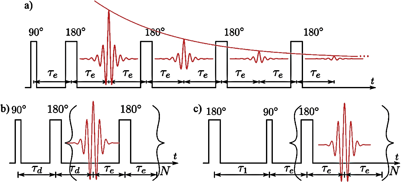
Fig. 2.
Pulse sequences used to measure: (a) the transverse relaxation times
4.A probehead for concurrent SANS and NMR measurements
As the sample cell is a critical parameter when it comes to study temperature driven critical phenomena (like the PMAA gelation process we are addressing in this study), great care has been taken to design a cell able to optimize the thermalization of the sample and in particular its equilibration time. In this section, we provide details on the specific sample cell manufactured for this work.
4.1.Design of a cell for in-situ NMR measurements on a SANS machine
To stay in tune with the classical soft matter conditions used on SANS spectrometer, the NMR-Neutron probehead has been designed to accommodate a classical
Fig. 3.
(a) picture of the NMR-neutron probehead (cover not shown). The copper NMR coil tightly surrounds a part of the Hellma® sample cell at immediate proximity of the neutron beam section. (b) 3D view of the probehead adaptation onto the NMR spectrometer. Here, the NMR-neutron probehead cover necessary to control the heated air stream used for the sample temperature regulation is shown.
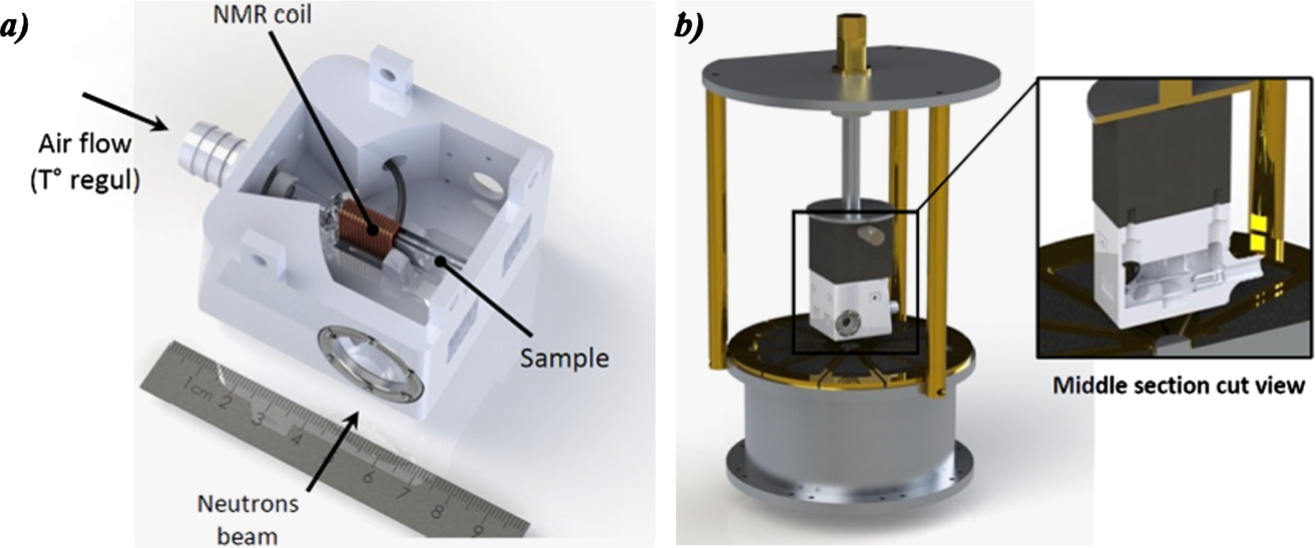
This Neutron-NMR probehead is shown on Fig. 3. It is made from PLA (polylactic acid) by 3D printing. It is closed to ensure the thermalization of the sample by a stream of heated air generated by a heat-gun and driven to the cell entrance by a standard plastic hose (see entrance funnel on Fig. 4). The neutron beam passes through two quartz windows. This geometry offers the large detector an angular access of 40° required for SANS measurements.
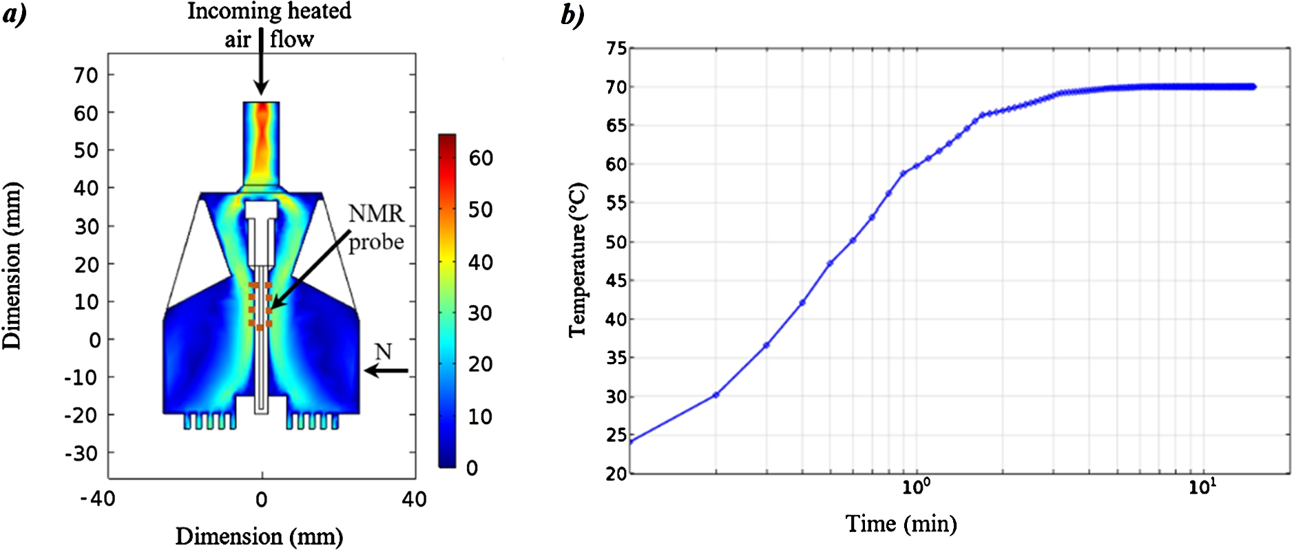
Fig. 4.
a) Simulation of the air-flow within the NMR-neutron probehead (sectional and top view). The color code (in
4.2.Optimization of the NMR-neutron probehead thermalization
To thermalize the sample, electric heating devices are usually used. Here, in order to avoid any magnetic field disturbances induced by electric current, we have chosen to use a stream of heated gas. The air stream within the NMR-Neutron cell has been simulated using the COMSOL® Multiphysics software. The simulations show that the air flow-rate is able to thermalize the sample (Fig. 4(a)). Experimentally, the sample temperature was directly measured inside the measuring cell using an optic fiber temperature sensor (OTG-M420, OpSens®) placed outside of the neutron beam cross-section. Starting from room temperature, when passing the set-point to 70°C, the required temperature is reached after 10 minutes and a stability within 0.1°C can be maintained for hours.We have checked that the sample temperature is not affected by overnight changes of ambient temperature in the neutron guide hall.
5.Coupling of the one-sided NMR system to the SANS machine
The adaptation of the one-sided NMR spectrometer on the SANS machine was rather straightforward. The major modification to the regular PAXY instrument set-up was the removal of the sample changer and of the goniometer usually installed underneath. This was necessary to minimize the interaction of the NMR magnet with such massive magnetic materials. To recover the proper position of the sample in the beam, these parts are replaced by pieces of high-density polyethylene. The hybrid NMR-SANS set-up is shown on Fig. 5.
6.Results
6.1.SANS
Small angle neutron scattering measurements have been performed at increasing temperature below and above the cloud point. At each temperature change, successive SANS spectra were measured for 5 minutes each, until no evolution of the scattering was detected. The equilibration of the sample was of the order of 30 minutes. The SANS data are shown on Fig. 6.
Fig. 5.
a) 3D model of the LLB SANS instrument PAXY. From right to left, the neutron guide (in turquoise blue), the one sided-NMR spectrometer (at the center of the picture on a) and b)) and the neutron detector box (zebra) are shown. b) Real picture of the central part modelized in a). The NMR magnet is seen in the middle of the picture and the NMR-neutron probehead is shown at the forefront. The copper NMR coil surrounding the Hellma® cell is set in place. The NMR console (not shown) was 2 meters away from the sample position.
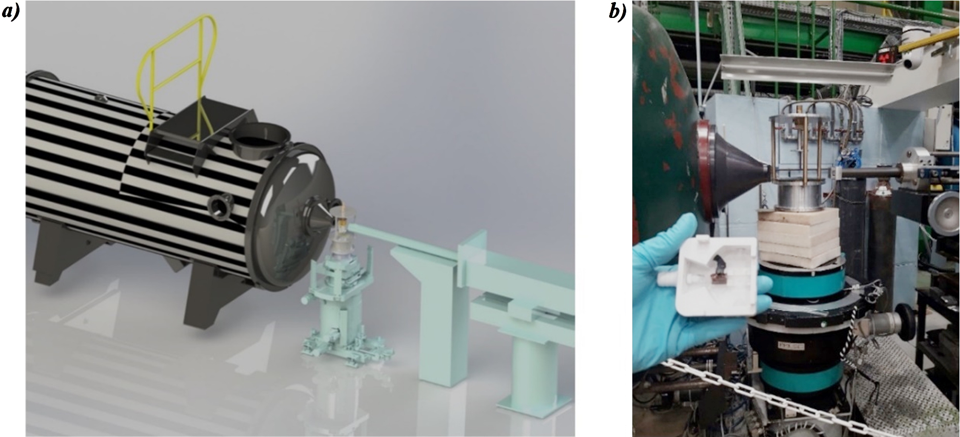
Fig. 6.
Scattering intensity of PMAA solution at
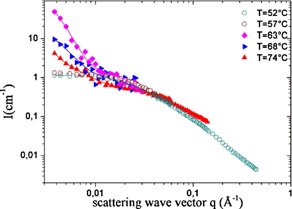
At low temperature, below the cloud-point, PMAA solutions behave as classical semi-diluted solutions. As shown on Fig. 6, the scattering intensity of PMAA solution at 80 g.l−1 can be fitted with a classical Ornstein–Zernike function:
Above the cloud-point, a strong intensity is detected at
After the phase transition,
Table 1
Interface area per volume of the 80 g.l−1 PMAA solution as a function of temperature. These values are obtained by a fit of data shown on Fig. 6 with Eq. (4)
| T (°C) | 52°C | 57°C | 63°C | 68°C | 74°C |
| S/V (mm−1) | 87 | 65 | 8 |
As clearly seen on Fig. 6, the
As the Ornstein–Zernike contribution remains very similar on the whole temperature range, we can consider to a good approximation that at the local scale the organization of the polymer chains is almost unaffected by the onset of the LCST transition.
The Ornstein–Zernike contribution is fitted at low temperature and is kept constant over the whole temperature range. The Eq. (4) then fits nicely the data on Fig. 6. Provided that upon an increase of temperature,
6.2.NMR
6.2.1.Relaxation times T 1 T 2
Figure 7 shows the curves obtained with the inversion-recovery experiments for different temperatures. In order to obtain the value of
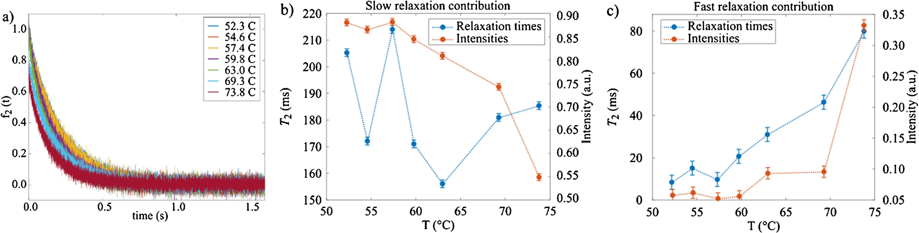
The transverse relaxation
Fig. 7.
NMR
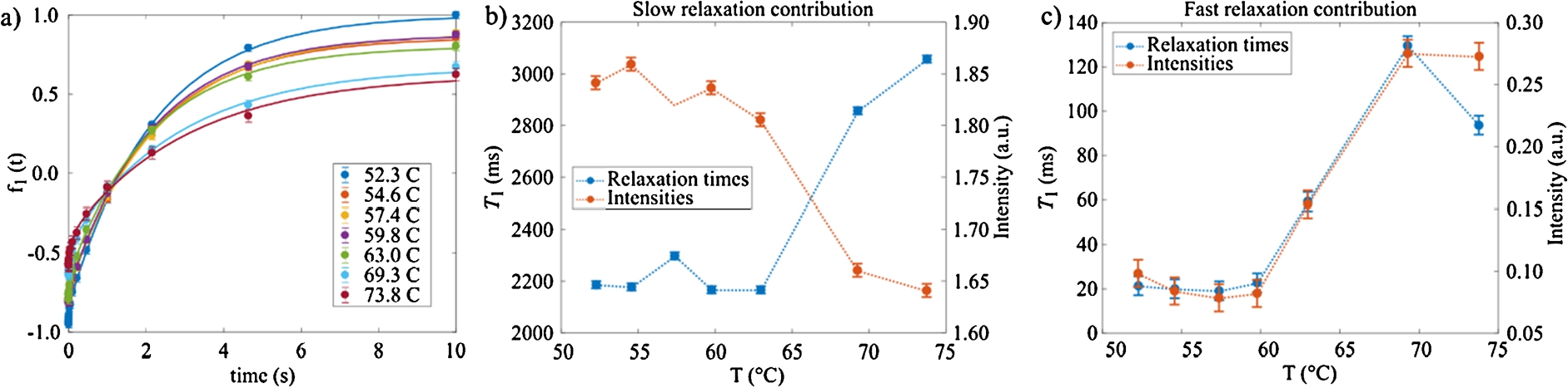
Fig. 8.
NMR
6.2.2.Self-diffusion coefficient experiments
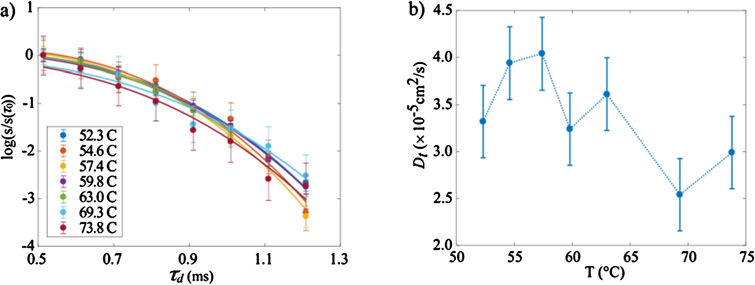
The results of the diffusion experiments as a function of temperature are shown on Fig. 9. These curves are determined by the intensities of the signal for each diffusion time
Fig. 9.
a) Diffusion curves obtained using the Hahn echo sequence as a function of the temperature. b) Self-diffusion coefficients of the protons of the system, determined by data fitting of data shown in a) according to Eq. (10).
7.Discussion
Using the bimodal NMR-SANS equipment described above, along with a regular SANS scattering instrument, we have been able to measure the common low field NMR parameters:
The gelation process we have been focusing on, is detected at the expected temperature of 65°C by SANS. Concomitant NMR measurements show the clear phase transition in the same temperature region. More specifically, abrupt changes of both T1 relaxations times are observed at this threshold temperature. The diffusion coefficient measured in these experiments may be compared with values in pure water [18] i.e.
Nevertheless, a thorough interpretation of the NMR data is challenging. First, here, the NMR signal is a composite information: both the protons from the solvent and from the PMAA contribute to the observed signal. Work is underway to find a way to better discriminate these two contributions. For future studies, a possible way out will be the use of fully deuterated water or PMAA.
At the present stage of development, we have made the choice i) to avoid any neutron beam-induced activation of the metallic (copper) NMR coil, ii) supress any parasitic SANS signal induced by the scattering of this coil and iii) eliminate any reproducibility issues due to a change of the coil position in the beam upon sample change. As a consequence, while they have been measured simultaneously and on the very same sample, the signal recorded by NMR and SANS were coming from slightly different volumes of the sample.
During the experiment, when increasing the sample temperature to reach the LCST region, we have noticed that the fraction of the sample embraced by the radiofrequency signal generated by the NMR coil, was showing critical opalescence few degrees before the expected gelation temperature. The fraction of the sample few millimetres away from this milky spot was actually perfectly transparent.
In the present study of a critical gelation phenomena, this localised opalescence can with not doubt be assigned only to a local increase of the temperature: the opalescent fraction of the sample has exceeded the LCST temperature while the transparent fraction remained below.
We therefore conclude that, even with a recyclable delay of 10 s for the NMR sequences pulses (0.16 s in the CPMG experiment and
To overcome local heating, so as to reach a uniform temperature over the whole sample volume, instead of measuring a steady sample enclosed in the cell, we could create a mild flow of the sample by circulating, in the cell, the sample from (and to) a mother reservoir. This microfluidic-like strategy seems an easy way to lift the issue of NMR coiled induced inhomogeneous heating of the sample, but is only adapted to liquids and/or low viscosity samples.
For solid or gels samples, a direct way to overcome the heating issue will be to position the NMR coil directly in the neutron beam. Such a setting takes advantage that in the SANS regime, most of the metallic materials show a moderate (but Q dependant) scattering. As copper activates with neutrons, a good coil material candidate would be aluminium (27 Al): its radioactive half-life being of 2 minutes, such a coil would have fully deactivated after a duration of the order of 20 minutes after the closure of the neutron beam.
In the future, the use of advanced NMR techniques, such as
8.Conclusion
In this paper, we have demonstrated that the coupling of a single-sided NMR system with a SANS instrument is experimentally possible. For this purpose, a home-made portable single-sided NMR setup was properly adapted to the SANS machine, and bimodal experiments were simultaneously carried out. The acquisition times needed to reach good signal to noise ratios, of the order of one hour for both NMR and SANS, match. Altogether, we show that the in-situ low-field NMR/SANS coupling the NMR is meaningful and is a promising experimental approach.
As both structural (
Such an in-situ SANS/NMR coupling experimental strategy is relevant in the field of chemical physics to finely probe systems like polymers, membranes, colloids in scientific fields spanning from geology (water management in soils, oil industry, etc.), electrochemistry (structural and related dynamical behaviours of electrolyte upon additives) to biophysics.
Acknowledgements
This project has received support from the program “Investissements d’Avenir” LabEx PALM (Project ANR-10-LABX-0039-PALM) and the Laboratoire Léon Brillouin (CEA-CNRS). This work was also supported by the Agence Nationale de la Recherche (ANR) under Grant NMR2GO (Grant ANR-06-JCJC0061), by the European Research Council under the European Community’s Seventh Framework Program (FP7/2007-2013), an ERC Grant agreement 205119 (R-EvolutioN-M-R), by the Research Foundation Flanders (FWO) under Grant PorMedNMR – n° G0D5419N and by LNCMI-CNRS, member of the European Magnetic Field Laboratory (EMFL). The authors are also thankful to Olivier Tessier and to Angelo Guiga for expert machining. The authors thank Pascal Lavie (LLB) for the 3D model shown on Fig. 5.
 This work was performed within the world class Science and Innovation with Neutrons in Europe 2020 (“SINE 2020”) project, funded by the European Commission, Grant Agreement n°65400.
References
[1] | M. Adam and D. Lairez, Sol-gel transition, in: Physical Properties of Polymeric Gels, J.P. Cohen Addad, ed., John Wiley & Sons, UK, (1995) , pp. 87–142. |
[2] | D. Lairez, De la physique des polymères vers des problèmes d’intérêt biologique, Habilitation à Diriger des Recherches, Université Paris Sud – XI., 2005. http://www-llb.cea.fr/habilitations/lairez-2005.pdf. |
[3] | E.R. Pike and J.B. Abbiss, Light Scattering and Photon Correlation Spectroscopy, Springer Science & Business Media, (2012) . |
[4] | F. Leclercq-Hugeux, M.-V. Coulet, J.-P. Gaspard, S. Pouget and J.-M. Zanotti, Neutrons probing the structure and dynamics of liquids, Comptes Rendus Phys. 8: ((2007) ), 884–908. doi:10.1016/j.crhy.2007.10.008. |
[5] | M.H. Levitt, Spin Dynamics: Basics of Nuclear Magnetic Resonance, John Wiley & Sons, (2001) . |
[6] | A. Silberberg and P.F. Mijnlieff, Study of reversible gelation of partially neutralized poly(methacrylic acid) by viscoelastic measurements, J. Polym. Sci. Part-2 Polym. Phys. 8: ((1970) ), 1089–1110. doi:10.1002/pol.1970.160080706. |
[7] | K. Nakamura, T. Itoh, M. Sakurai and T. Nakagawa, The viscoelastic properties of aqueous poly(methacrylic acid) solutions and their relations to thermoreversible gelation, Polym. J. 24: ((1992) ), 1419. doi:10.1295/polymj.24.1419. |
[8] | M. Sakurai, T. Imai, F. Yamashita, K. Nakamura, T. Komatsu and l.T. Nakagawa, Temperature dependence of viscosities and potentiometric titration behavior of aqueous poly(acrylic acid) and poly(methacrylic acid) solutions, Polym. J. 25: ((1993) ), 1247–1255. doi:10.1295/polymj.25.1247. |
[9] | J. Eliassaf, Aqueous solutions of poly(N-isopropylacrylamide), J. Appl. Polym. Sci. 22: ((1978) ), 873–874. doi:10.1002/app.1978.070220328. |
[10] | A. Meier-Koll, V. Pipich, P. Busch, C.M. Papadakis and P. Müller-Buschbaum, Phase separation in semidilute aqueous poly(N-isopropylacrylamide) solutions, Langmuir. 28: ((2012) ), 8791–8798. doi:10.1021/la3015332. |
[11] | C. Robin, C. Lorthioir, C. Amiel, A. Fall, G. Ovarlez and C. Le Cœur, Unexpected rheological behavior of concentrated poly(methacrylic acid) aqueous solutions, Macromolecules. 50: ((2017) ), 700–710. doi:10.1021/acs.macromol.6b01552. |
[12] | Spectromètre de diffusion aux petits angles PAXY, (n.d.), http://www-llb.cea.fr/spectros/spectro/paxy.html. |
[13] | F. Casanova, J. Perlo and B. Blümich, Single-Sided NMR, Springer Science & Business Media, (2011) . |
[14] | C. Hugon, G. Aubert and D. Sakellariou, A systematic approach to the design, fabrication and testing of permanent magnets applied to single-sided NMR, AIP Conf. Proc. 1330: ((2011) ), 105–108. doi:10.1063/1.3562244. |
[15] | C. Hugon, G. Aubert and D. Sakellariou, An expansion of the field modulus suitable for the description of strong field gradients in axisymmetric magnetic fields: Application to single-sided magnet design, field mapping and STRAFI, J. Magn. Reson. San Diego Calif 1997 214: ((2012) ), 124–134. doi:10.1016/j.jmr.2011.10.015. |
[16] | K.S. Panesar, C. Hugon, G. Aubert, P. Judeinstein, J.-M. Zanotti and D. Sakellariou, Measurement of self-diffusion in thin samples using a novel one-sided NMR magnet, Microporous Mesoporous Mater. 178: ((2013) ), 79–83. doi:10.1016/j.micromeso.2013.04.016. |
[17] | P. Judeinstein, F. Ferdeghini, R. Oliveira-Silva, J.M. Zanotti and D. Sakellariou, Low-field single-sided NMR for one-shot 1D-mapping: Application to membranes, J. Magn. Reson. 277: ((2017) ), 25–29. doi:10.1016/j.jmr.2017.02.003. |
[18] | M. Holz, S.R. Heil and A. Sacco, Temperature-dependent self-diffusion coefficients of water and six selected molecular liquids for calibration in accurate 1H NMR PFG measurements, Phys. Chem. Chem. Phys. 2: ((2000) ), 4740–4742. doi:10.1039/B005319H. |

