
Long short-term memory stacking model to predict the number of cases and deaths caused by COVID-19
Abstract
The long short-term memory (LSTM) is a high-efficiency model for forecasting time series, for being able to deal with a large volume of data from a time series with nonlinearities. As a case study, the stacked LSTM will be used to forecast the growth of the pandemic of COVID-19, based on the increase in the number of contaminated and deaths in the State of Santa Catarina, Brazil. COVID-19 has been spreading very quickly, causing great concern in relation to the ability to care for critically ill patients. Control measures are being imposed by governments with the aim of reducing the contamination and the spreading of viruses. The forecast of the number of contaminated and deaths caused by COVID-19 can help decision making regarding the adopted restrictions, making them more or less rigid depending on the pandemic’s control capacity. The use of LSTM stacking shows an R2 of 0.9625 for confirmed cases and 0.9656 for confirmed deaths caused by COVID-19, being superior to the combinations among other evaluated models.
1Introduction
Recently the new coronavirus (SARS-CoV-2) proved to be a highly contagious virus, considering that it soon spread throughout the world and caused serious consequences to the health of the population [1]. Due to easy contagion, certain restrictive measures were imposed in Brazil to prevent the virus from spreading widely and generate catastrophic consequences on public health. One of the main concerns is that the health system is unable to receive and treat all patients properly [2].
SARS-CoV-2 causes the disease COVID-19, which presents a clinical picture that can range from asymptomatic infections to severe respiratory conditions, which in the absence of treatment can cause death [3]. According to the World Health Organization (WHO), most patients with COVID-19 can be asymptomatic, which makes it difficult to identify where the virus is spreading [4].
Some patients with COVID-19 may require hospital care with support for the treatment of respiratory failure, which makes it necessary to have an adequate forecast for the increase of cases [5]. From a forecast it is possible to have control of restrictive measures, in relation to the capacity of advanced treatments [6]. Based on this need, this article aims to assess the ability to predict deaths and infections in the state of Santa Catarina in southern Brazil, in order to indicate whether restrictive measures are generating efficient results.
Some authors have carried out works related to the evaluation of the spread of viruses and the ability to predict this disease. In the work of Pinto, Nepomuceno and Campanharo a study is presented on the spread of infectious diseases [7]. The evaluation shows that complex networks result in curves of infected individuals with different behaviors and, therefore, the growth of a given disease is highly sensitive to the model used. In [8] published reports on forecast models for the diagnosis of COVID-19 in patients with suspected infection are analyzed. In this study, the ability to detect people in the general population at risk of being admitted to the hospital for pneumonia is assessed.
Al-qaness et al. [9] present in their study a new model that aims to predict 10 days in advance the number of confirmed cases of COVID-19 using as a basis the cases previously registered in China. For that, they used an adaptive neuro-fuzzy inference system model (ANFIS). In comparison with other existing models, ANFIS showed better performance in calculating error and computational effort.
Sajadi et al. [10] conducted a study in which climate data from cities with significant community dissemination of COVID-19 were examined using retrospective analysis. So far, there has been significant community dissemination in cities and regions with similar weather patterns with average temperatures in the range of 5-11°C and humidity between 4-7g/m3 The outbreak distribution in regions with these climatographic characteristics is consistent with a seasonal respiratory virus.
Fanelli e Piazza [11] present an analysis of the spread of COVID-19 in China, Italy and France. In this work they mention that in an initial analysis of day-lag graphs, the results show that it is possible to identify a simple model to understand the spread of the epidemic, height and time to reach the peak of the curve of confirmed infected individuals. The analysis also shows that the recovery rate follows the same kinetics regardless of the country under analysis, while the rates of infection and death vary. A simulation of the effects of drastic measures to contain the outbreak in Italy shows that a reduction in the rate of infection actually causes an attenuation of the peak of the epidemic, and it is also observed that the rate of infection needs to be reduced dramatically and quickly to see a noticeable decrease in the epidemic peak and mortality rate.
Roosa et al. [12] used in their research phenomenological models already validated for a short-term forecast of the cases reported in Guangdong and Zhejiang, China. It was possible to make a 5 and 10 day forecast using accumulated data collected from the National Health Commission of China until February 13, 2020. For this, the researchers used a generalized logistic growth model, Richards’ growth models and a sub-epidemic wave model that had previously been used to predict outbreaks of infectious diseases at other times. By using 3 models it was possible to obtain a forecast, using the 10-day condition, of 65 to 81 additional cases in Guangdong and 44 to 354 cases in Zhejiang. It can be seen with this that the transmission in both cities is showing a decrease.
In the article by He, Tang and Rong [13], a short-time stochastic epidemic model with binomial distribution was presented for the study of coronavirus transmission. The model parameters were adjusted based on data collected in China between 11 and 13 February 2020. The estimates of the contact rate and the effective number of reproduction indicate the efficiency of the control measures when applied quickly. The simulations show that the total number of confirmed cases peaked at the end of February 2020, considering that the applied control measures were maintained. Although the number of new cases of infection is decreasing, there is still the possibility of future outbreaks if adequate protective measures are not taken.
There are several algorithms that can be used to forecast time series. Choosing the best model [14] and configuration [15] can improve the predictability of the algorithm. In the article [16] the forecast is made through a neuro-fuzzy network with success for a short-term time series. In [17], several ways of using the Ensemble algorithm are applied to the short-term forecasting problem. The use of optimization methods and hybrid algorithms is also a promising alternative to assess the problem [18].
Time series forecasting is applied to several areas of knowledge, some works stand out for this purpose using advanced forecasting techniques. In [19] the least squares support vector machine classifier combined to chaotic cloud particle swarm optimization is applied to forecasting ship motion, in [20] and [21] a hybrid model is used for forecasting energy consumption, Zhang and Hong [22] used a combined model for the same purpose. In [23] a combination of models is performed to improve the predictability of the algorithm. Papers [24] and [25] perform the prediction based on a support vector regression model.
Among the algorithms for the prediction of time series [26–28], neural networks with deep learning have gained space for the time series forecasting of COVID-19 spread [29–32], considering that they have the capacity to analyze a large volume of data with non-linearities. Long short-term memory (LSTM) is a recurrent neural network (RNN) that can process entire sequences of data, making this algorithm suitable for the problem in question [33]. The insensitivity regarding the gap length gives the LSTM an advantage over traditional RNNs and classic approaches, such as nonlinear auto-regressive algorithms.
The use of stacked LSTM is promising for time series forecasting [34]. Stacking the layers can improve the model’s ability to capture temporal dependency patterns. According to Liang et al. [35] stacked LSTM is suitable to perform wind speed prediction for wind power producers and grid operators. The results show that this type of model has the ability to capture and learn uncertainties at the same time that it presents an output performance.
The stacked LSTM model has applications in several areas, and it can even be used to forecast stock prices in the financial market. According to Xu et al. [36], the use of wavelet transformation reduces noise and improves the predictive capacity of the model. Bao et al. [37] presents a work with the same objective-based on stacked autoencoders, the results show that this approach is superior to other predictive models.
In this paper, the stacked LSTM model was used because it has the ability to handle non-linear data. The measurement of cases may vary due to the under-reporting of cases on weekends and variation in the weekly work schedules of the health teams. This variation can cause peaks of cases, not representing the actual situation of the pandemic. For this reason, the forecasting model needs to be able to interpret non-linear data.
The contributions of this paper to predict the number of cases and deaths caused by COVID-19 are summarized in the following:
- The first contribution is the forecast of an increase in cases and deaths caused by COVID-19 in Santa Catarina, Brazil. Based on a reliable forecasting model, it is possible to define strategies to minimize the impact of the pandemic caused by COVID19;
- The second contribution focuses on use of a deep learning model with layers stacked. This network structure is robust to deal with non-linear data, improving the quality of time series prediction;
- The third contribution is related to the evaluation of all network parameters to improve the model. Through optimized parameters, a model with greater capacity to deal with the problem is obtained.
In this article the stacked LSTM will be used to assess the ability to predict contagion and the evolution of the number of deaths caused by COVID-19, using the State of Santa Catarina (Brazil) as a case study. In Section 3 the proposed method will be explained. In Section 2 the problem related to the virus will be presented. In Section 4 the results of the analysis will be discussed. Finally, Section 5 will present the conclusions of this article.
2Case study
The World Health Organization officially called the disease caused by the coronavirus COVID-19 [38]. The number 19 refers to the year 2019 when the first cases in Wuhan (China) were publicly disclosed. The name Corona refers to the shape of the virus that resembles the shape of a crown, Figure 1 presents an illustrative image of the Coronavirus (SARS-CoV-2 virus) [39].
![Ilustration of the SARS-CoV-2 virus [4].](https://ip.ios.semcs.net:443/media/ifs/2022/42-6/ifs-42-6-ifs212788/ifs-42-ifs212788-g001.jpg)
COVID-19 is an infectious disease caused by the recently discovered coronavirus. The virus is highly contagious, being transmitted through droplets generated when an infected person coughs, exhales, or sneezes [40]. The droplets are weighed and are thus quickly deposited on surfaces that remain infected for a long time. A person can become infected with COVID-19 by inhaling the virus if they are close to someone infected or by touching a contaminated surface and rubbing their hands over their nose, eyes, or mouth [41].
2.1Contamination in the Santa Catarina state
To reduce the contagion of COVID-19, the Government of the State of Santa Catarina, through Provisional Measure No. 227 of 2020, established measures to deal with public calamity and the public health emergency resulting from COVID-19. Among the measures adopted, remote work was adopted when possible, there was anticipation of vacations and leave for public servants [42].
In addition to Provisional Measure No. 227 of 2020, there have been several decrees aimed at reducing contagion by the coronavirus. Among the measures adopted based on these decrees, some commercial activities were closed at the beginning of the pandemic, events with crowds of people were banned and it was mandatory to use masks indoors [43].
Despite the great public health effort and the restrictive measures imposed by the Government of the State of Santa Catarina (SC), the cases of COVID-19 continue to increase. In Figure 2 can be viewed the locations in the state where there is confirmation of cases.
![Confirmed cases of COVID-19 in SC [44].](https://ip.ios.semcs.net:443/media/ifs/2022/42-6/ifs-42-6-ifs212788/ifs-42-ifs212788-g002.jpg)
Mass testing of COVID-19 cases has not yet been possible, so only professionals directly involved in combating COVID-19 are tested or patients who have very clear symptoms of the disease. The number of deaths in relation to the number of contaminated is considerably large compared to places where mass population testing was carried out, as can be seen in Figure 3. The cities with the largest number of inhabitants had a higher number of contaminated ones, with many confirmed cases in the cities of Florianópolis, Chapecó, Blumenau, Joinville and Criciúma. The highest number of deaths in the state was registered in the cities of Florianópolis, Joinville and Criciúma [44].
![Deaths confirmed by COVID-19 in SC [44].](https://ip.ios.semcs.net:443/media/ifs/2022/42-6/ifs-42-6-ifs212788/ifs-42-ifs212788-g003.jpg)
The evolution of the number of confirmed infected cases and death records is used in this article to train the neural network and to forecast the continuity in the spread of the virus. The data used to analyze the proposed algorithm, are based on official records informed by the Government of the State of Santa Catarina.
3Methodology
LSTM is a recurrent neural network algorithm. Unlike common neural networks that have the feedforward form, LSTM has feedback allowing the algorithm to remember distant values [45]. With LSTM, P steps forward, starting from D samples, sampled in an interval Δ,
(1)
(2)
For this, the classic LSTM algorithm is composed of cells that repeat themselves, as can be seen in Figure 4. Each cell is divided into three gates, the entrance (it), exit (ot) and the forgetting (ft) gates. These gates regulate how much of the respective variable will be sent to the next step [46].
Fig. 4
LSTM cell.
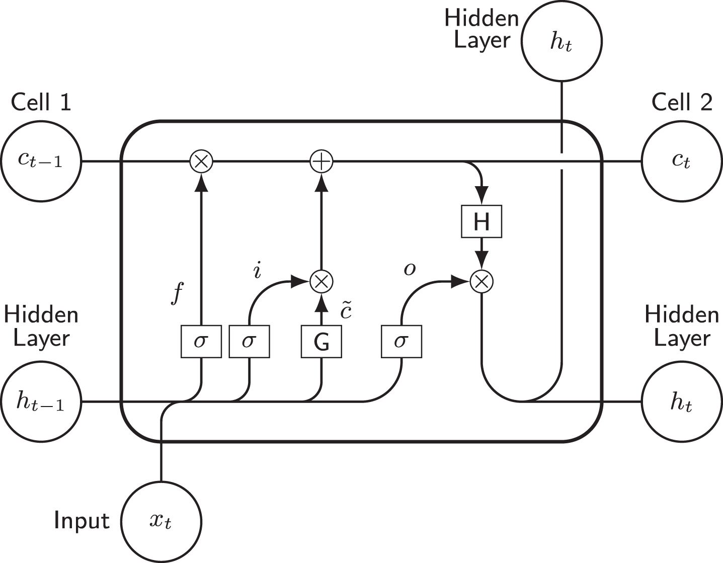
The first gate, of forgetting (forget), determines how much of the information passed will be forgotten and how much will be remembered [47]. Useful information for states is added via the input gate (input), the input values are activated by an activation function. Finally, at the output gate (output) it is determined how much of the current state should be assigned to the output [48]. For this, the current state is activated and regulated by the input. In terms of the equation, the LSTM can be expressed by the equations:
(3)
Where W and R are earnings matrices and b the polarization matrix, whose values will be assigned by the network training. For these equations σg denotes the activation function of gate. LSTM has the input activation function G and the output activation function H of the cell, (see Figure 4) which are used to update the cell and the hidden state, according to the equations:
(4)
The operations are performed element by element, and ∘ circ represents the product of the elements. To perform the forecast values of the stages of future time, the responses of the training sequences are displaced by a time step. In this way, at each time step of the input sequence, the network learns to predict the value of the next time step [49].
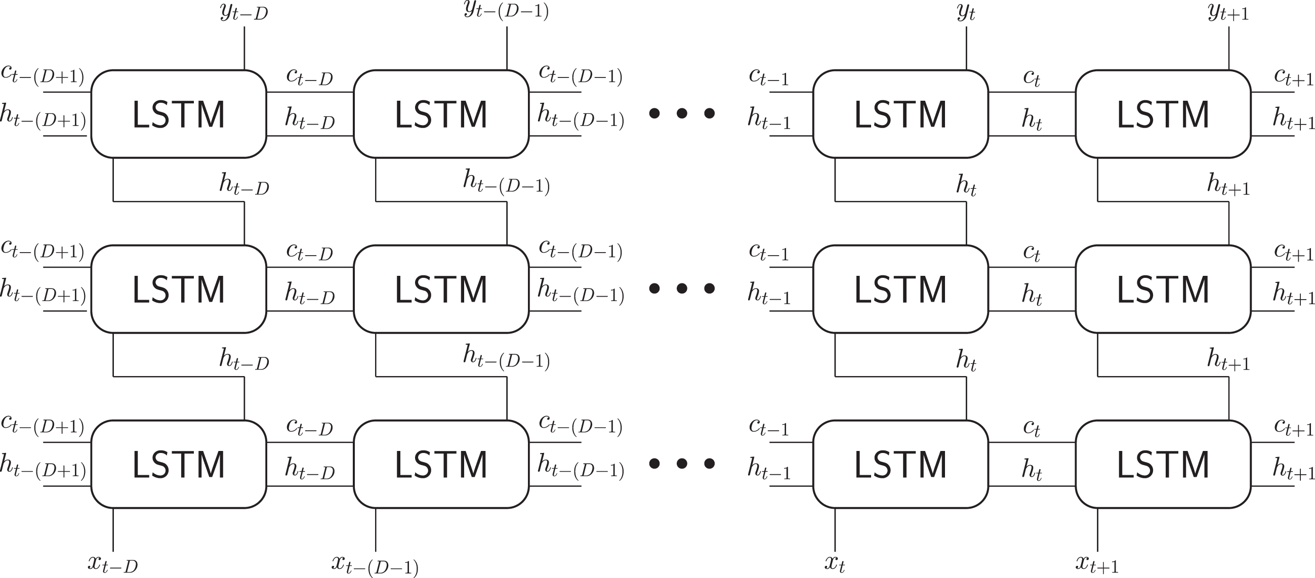
In this article the LSTM layers are included in the algorithm in a stacked way [50], as seen in Figure 5, based on each cell presented in Figure 4. Stacked LSTM is an extension of this model that has several hidden layers of LSTM, where each layer contains multiple memory cells [48]. For complete evaluation of the algorithm, the regression can be specified with variations in the number of layers, activation function, number of hidden units and optimization method.
Fig. 5
LSTM stacking scheme using 3 layers.
In this article, the activation functions linear, sigmoid, hyperbolic tangent, rectified linear unit, exponential linear unit and SoftPlus were evaluated. The linear function can be ideal for simple tasks, since its derivative is constant, that is, it does not depend on the input value.
The sigmoid activation function (Sigm) is a widely used function, as it is smooth and continuously differentiable. The hyperbolic tangent activation function (TanH) is similar to the sigmoid function, being a scaled version of this function [15]. The rectified linear unit (ReLU) function is being widely used nowadays to deep learning approaches. A similar activation function to ReLU is the exponential linear unit (ELU) function [51].
To improve the performance of the algorithm, the optimizer must also be evaluated. The stochastic gradient descent (SGD) algorithm, updates the neural network parameters to minimize the loss function, taking small steps in each iteration towards the negative loss gradient. RMSProp uses learning rates that differ by parameter and can automatically adapt to the loss function being optimized [49]. Thus, the algorithm maintains a moving average of the squares of the elements of the parameter gradients. This algorithm uses this moving average to normalize the updates for each parameter individually.
The Adaptive Moment Estimation (ADAM) optimization method calculates adaptive learning rates for each parameter [52, 53]. ADAM uses moving averages to update network parameters. AdaMAX algorithm is a variant of ADAM optimizer based on the infinity norm. The AdaMAX can be promissor specially in embedded models. The Nesterov accelerated adaptive moment estimate (NADAM) is a combination of the Adam method and the Nesterov accelerated gradient (NAG). The NADAM optimizer is used to minimize the cross entropy loss function [54].
AdaGRAD, is based on the gradient that adapts the learning rate to the parameters [55]. AdaGRAD performs minor updates to parameters associated with frequently occurring resources; and performs major updates to parameters associated with infrequent resources. AdaDELTA is an extension of AdaGRAD that seeks to reduce its decreasing learning rate. Instead of accumulating all the previous square gradients, AdaDELTA restricts the gradient window to a fixed size. The current average depends only on the previous average and the current gradient [49].
3.1Algorithm evaluation
For evaluation of the algorithm using a quantitative methodology [56], a metric of the global error evaluation based on the Root Mean Square Error (RMSE) is used for network training and testing procedures. The error signal is calculated by the difference between the goal of the yi network and the result of the
(5)
Other measures to calculate the error are also presented to evaluate the proposed method, such as the Mean Absolute Error (MAE), and the Mean Absolute Percentage Error (MAPE) [58]. These measures are calculated according to the equations:
(6)
(7)
MAPE calculates the average error rate for the correct values and MAE is the mean of the absolute difference between the observed and predicted values [59]. Based on recent studies on the application of time series forecasting, the R2 determination coefficient is a promising way to assess model performance [60, 61].
(8)
In this case,
(9)
(10)
(11)
In equations (9 and 10), yi,p is the value of the predicted output i in object p and
For a final comparison of the algorithm a benchmarking was performed. In this evaluation the layers were combined for a complete comparison. Recurrent neural network (RNN), gated recurrent unit network (GRU), simple recurrent neural network (SRNN), and dense structures were used for comparison [64].
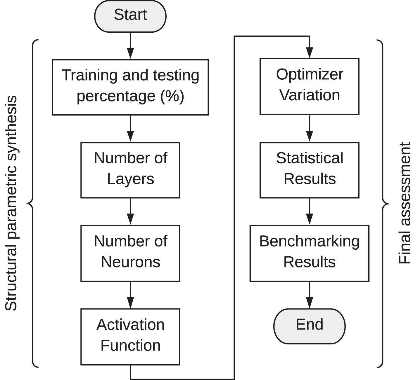
This article will evaluate network performance using an AMD Ryzen 5 (model 3400G) computer Quad-Core 3.7 GHz, with 8.00 GB of random-access memory (RAM), double data rate (DDR) 4. The algorithm was developed using the Python language from the Keras package based on TensorFlow. The complete flowchart of the steps performed in the analysis of the model used in this paper is presented in Figure 6.
Fig. 6
Flowchart of the procedure performed in this paper.
4Results analysis
In this section, the analysis of the proposed method will be presented. Initially, the prediction capacity in relation to the size of dataset needed to perform the training of the neural network will be evaluated, considering the RMSE and the R2 of the algorithm. To assess R2, the determination coefficient will be used. Results with lower RMSE and higher determination coefficient will be highlighted in bold. Then the number of neurons and layers for the analyzed model will be evaluated. The results of applying various activation functions and methods of network optimization will also be presented. Finally, a statistical analysis will be performed based on the best configuration for the analyzed model.
The evaluation of the model is performed for the number of confirmed deaths, and based on the best configuration of the model, statistical analysis will be performed for the number of cases. For comparative purposes, the tests started with the SoftPlus activation function, 40 neurons and 1 step predicted ahead, from 30 samples. In this initial analysis, the ADAM optimizer was used from 90 % of the data for network training. This initial configuration was based on [14], in which variations are evaluated for the best configuration of the model. In this article the layers are organized by stacking cells, as explained in Section 3. Table 1 presents the results in relation to the variation in the size of data used for training. In this model, cross-validation is performed, in which the data used for training are not used for the network test.
Table 1
Results for Size (%) of Data Used for Training
| % | Train. (s) | RMSE | MAE | MAPE | R2 |
| 90 | 6.3 | 4.6×10² | 3.9×10² | 0.02 | 0.99 |
| 80 | 9.7 | 3.4×10³ | 3.1×10³ | 0.18 | 0.16 |
| 70 | 10.3 | 3.0×10³ | 2.4×10³ | 0.14 | 0.61 |
| 60 | 5.9 | 1.0×10⁴ | 9.1×10³ | 0.58 | 0.98 |
| 50 | 7.0 | 2.4×10⁴ | 1.6×10⁴ | 0.97 | 0.80 |
| 40 | 5.2 | 7.5×10⁴ | 4.7×10⁴ | 3.08 | 0.77 |
Using 90 % of the data for training the network, it is possible to achieve an R2 of 0.9943 to forecast the number of confirmed cases with COVID-19. This value is calculated based on the cross-validation of the data that are used for the training (data reported by the State Government), in relation to the forecast result.
It is possible to observe in Table 2 that the best stacking of this model occurs with 5 layers. From this result, the simulations were repeated to assess the influence of different numbers of neurons, according to Table 3.
Table 2
Results for Variation in the Number of Layers
| Lay. | Train. (s) | RMSE | MAE | MAPE | R2 |
| 1 | 10.0 | 3.3×10³ | 2.9×10³ | 0.16 | 0.54 |
| 2 | 10.5 | 6.5×10³ | 5.3×10³ | 0.29 | 0.94 |
| 3 | 12.8 | 2.8×10³ | 2.4×10³ | 0.13 | 0.97 |
| 4 | 16.4 | 1.3×10³ | 1.1×10³ | 0.06 | 0.84 |
| 5 | 17.3 | 1.6×10³ | 1.3×10³ | 0.07 | 0.97 |
| 6 | 31.0 | 6.8×10³ | 5.5×10³ | 0.30 | 0.95 |
Table 3
Results for Variation in the Number of Neurons
| Neur. | Train. (s) | RMSE | MAE | MAPE | R2 |
| 1 | 35.4 | 1.4×10⁴ | 1.4×10⁴ | 0.79 | nan |
| 5 | 19.4 | 1.5×10⁴ | 1.4×10⁴ | 0.80 | 0.02 |
| 10 | 51.1 | 1.5×10³ | 1.2×10³ | 0.07 | 0.80 |
| 20 | 26.9 | 1.4×10³ | 1.2×10³ | 0.06 | 0.81 |
| 30 | 19.6 | 3.0×10³ | 2.5×10³ | 0.13 | 0.99 |
| 40 | 17.9 | 4.8×10³ | 3.9×10³ | 0.21 | 0.97 |
| 50 | 45.6 | 3.9×10³ | 3.2×10³ | 0.17 | 0.95 |
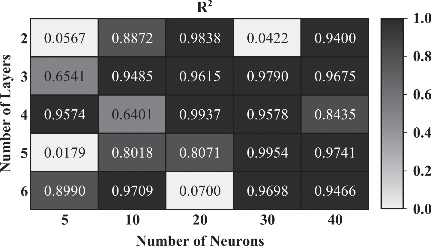
The best performance of the model was obtained using 30 neurons, resulting in lower errors and less time needed for training. The evaluation of the parameters in relation to the R2 of the model is presented in Figure 7 with greater precision, with all combinations between the number of neurons and the number of layers.
Fig. 7
Analysis of parameters variation.
In the Table 4 the results are presented in relation to the use of different activation functions and the Table 5 presents the results in relation to the variation in the use of the optimization method.
Table 4
Results for Varying the Activation Function
| Activ.Funct. | Train. (s) | RMSE | MAE | MAPE | R2 |
| Linear | 21.39 | 7.7×10³ | 5.0×10³ | 0.27 | 0.49 |
| Sigm | 27.55 | 1.8×10⁴ | 1.8×10⁴ | 1.00 | 0.01 |
| SoftPlus | 15.12 | 1.1×10⁴ | 8.5×10³ | 0.46 | 0.93 |
| TanH | 15.43 | 1.8×10⁴ | 1.8×10⁴ | 1.00 | 0.01 |
| ReLU | 29.86 | 1.2×10² | 8.3×10² | 0.01 | 0.99 |
| ELU | 13.50 | 8.6×10³ | 7.0×10³ | 0.38 | 0.95 |
The best results in terms of RMSE reduction and higher determination coefficient were obtained using the ReLU activation function. Changing the optimizer applied to the problem resulted in large variations in the R2 of the forecast. In this evaluation, RMSprop and SGD had results below the average of the other methods. The optimizer that resulted in the best R2 was ADAM, which also had the smallest error in all the metrics evaluated.
Table 5
Results for the Optimizer Variation
| Optim. | Train. (s) | RMSE | MAE | MAPE | R2 |
| SGD | 8.5 | 1.8×10⁴ | 1.8×10⁴ | 1.00 | 0.00 |
| ADAM | 31.1 | 4.8×10² | 4.1×10² | 0.02 | 0.99 |
| NADAM | 69.4 | 4.0×10³ | 3.3×10³ | 0.18 | 0.96 |
| RMSprop | 15.6 | 8.5×10² | 6.2×10² | 0.03 | 0.33 |
| AdaDELTA | 166.3 | 1.6×10⁴ | 1.6×10⁴ | 0.84 | 0.54 |
| AdaGRAD | 25.0 | 2.3×10³ | 2.1×10³ | 0.11 | 0.98 |
| AdaMAX | 11.7 | 3.2×10³ | 2.9×10³ | 0.16 | 0.97 |
Based on the analyzes presented here, the configuration that generated the best result in terms of greater precision and less error was with 90 % of the data for network training, 5 layers and 30 neurons. The best activation function was the ReLU and the best optimizer for the analysis of this paper was ADAM. From this configuration, a statistical evaluation based on 50 simulations is presented in 4.1 to assess the forecast of the number of confirmed cases and number of deaths.
From this configuration, Figure 8 shows the relationship between the increase in the real number of cases [43], obtained based on official information, training data and forecasting the evolution of cases. The assessment is presented after the first day on which a case of COVID-19 was confirmed in the state.
Fig. 8
Analysis of the Evolution of the Number of Cases.
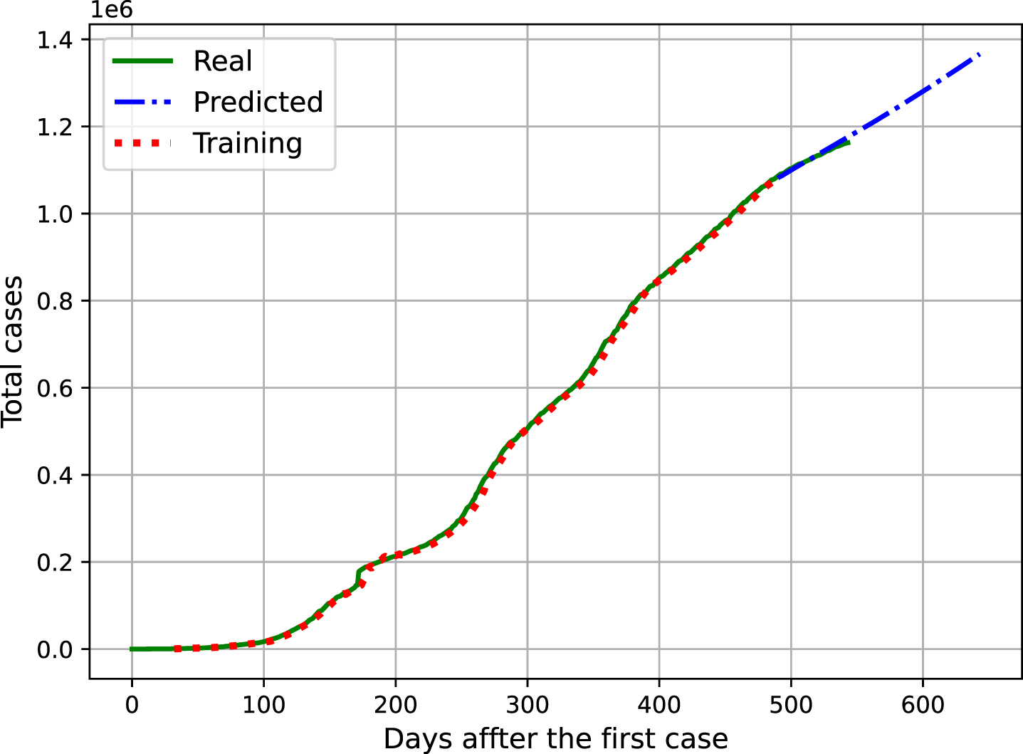
In this visual analysis, the values presented are real for confirmed cases (Real), those used for network training (Training) and the time series forecast (Predicted). Based on this analysis, it is possible to assess the trend in the increase in the number of cases in the future.
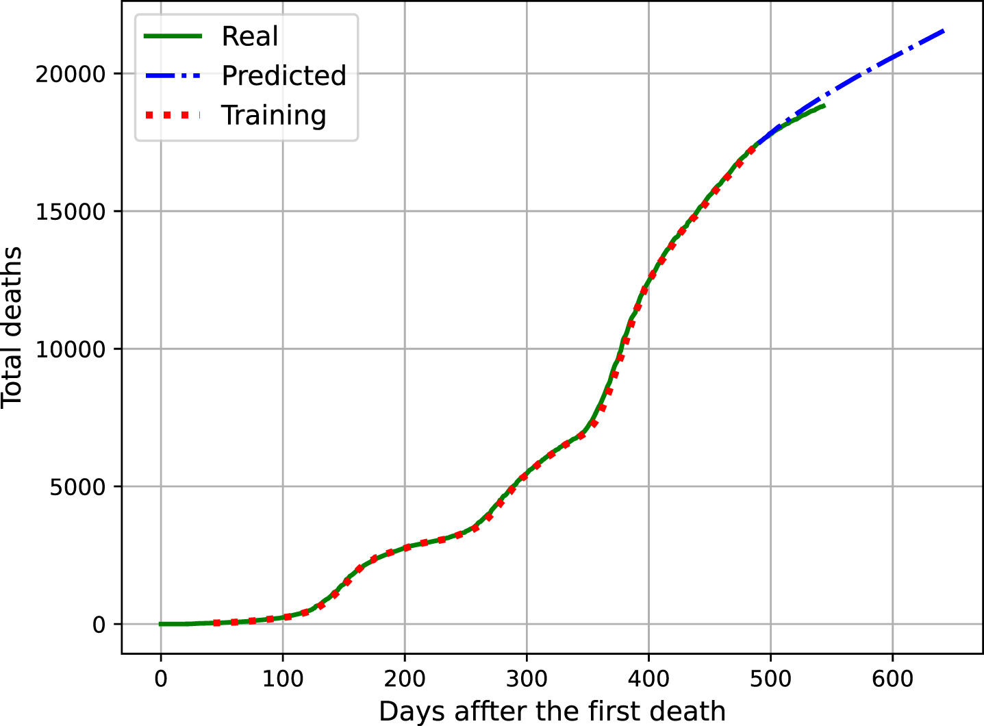
This evaluation shows that the increase in the number of cases in the coming days tend to grow slowly possibly stabilizing at a value. That’s given the vaccination advances and the restrictive measures. The same analysis is presented for the number of deaths confirmed by COVID-19 in Figure 9. There is a slightly higher growth but still a concave curve, this analysis shows the effects that vaccination had and will have in controlling the spread of the virus.
Fig. 9
Analysis of the Evolution of the Number of Deaths.
4.1Statistical analysis
For the final assessment the statistical analysis of the algorithm is performed, Table 6 presents a complete statistical analysis of 50 simulations with the same configuration described on previous section for confirmed cases and Table 7 for the number of deaths caused by COVID19. The statistical analysis shows that the variation of the values is low for the calculation of RMSE, MAE, MAPE, and R2.
Table 6
Statistical Results of the Proposed Method for Confirmed Cases
| Indicator | Training Time (s) | RMSE | MAE | MAPE | R2 |
| Mean | 28.23 | 1.72×10⁵ | 1.46×10⁵ | 0.12804 | 0.9077 |
| Std. Dev. | 10.58 | 2.19×10⁵ | 2.05×10⁵ | 1.82×10⁻¹ | 1.96×10⁻¹ |
| Variance | 111.86 | 4.78×10¹⁰ | 4.22×10¹⁰ | 3.32×10⁻² | 3.83×10⁻² |
Table 7
Statistical Results of the Proposed Method for Confirmed Deaths Caused by COVID-19
| Indicator | Training Time (s) | RMSE | MAE | MAPE | R2 |
| Mean | 23.22 | 2.69×10³ | 2.19×10³ | 0.1887 | 0.8861 |
| Std. Dev. | 7.58 | 2.28×10³ | 1.86×10³ | 1.01×10⁻¹ | 2.00×10⁻¹ |
| Variance | 57.4 | 5.20×10⁶ | 3.46×10⁶ | 1.02×10⁻² | 3.99×10⁻² |
As can be seen, there is a great variation in the results as a function of the magnitudes of the metric considered. This result does not represent a problem for the analysis, since the error remains under 1 % of the maximum order of magnitude of the metric used.
The R2 average found in this analysis remained at 0.9077 for number of confirmed cases, which shows that even with several analyzes the precision remains at a high average and the error calculated by RMSE, MAE and MAPE were low. The values of standard deviation and variance of RMSE and MAE were high, these results were obtained because the signal features which results in a greater error. Even with a longer time to start in the increase of confirmed deaths, the forecast remains accurate. In this way, it is possible to estimate the number of deaths caused by COVID-19, if the same measures to combat the virus are being taken.
The R2 achieved for predicting the number of deaths reaches 0.8861 from the average of 50 simulations, according to the determination coefficient R2. Based on the R2 found in this paper, it is possible to perform a strategic planning to combat COVID-19. This planning can be based on the results values found of the forecast of increases in confirmed cases and deaths.
In the subsection 4.2, to perform a fairer assessment using the same data set and with the same configurations, the results of the application of the GRU, Dense and SRNN models are compared to the LSTM stacking model.
4.2Benchmarking
In Table 8 variations of the model structure for the prediction of the increase of the confirmed cases of COVID-19 are presented. It is possible to observe that some layers structures do not generate acceptable R2 with results lower than 80 %. All the structures have higher error and low accuracy than the proposed method. The results of the evaluation for the number of deaths confirmed by COVID-19 was follows this tendency, as shown in Table 9.
Table 8
Benchmarking Results for Confirmed Cases
| Algorithm | Train Time (s) | RMSE | MAE | MAPE | R2 |
| GRU_GRU | 12.31 | 7.7×10⁵ | 5.5×10⁵ | 0.4835 | 0.7252 |
| GRU_SRNN | 27.61 | 3.0×10⁴ | 2.3×10⁴ | 0.0204 | 0.4482 |
| GRU_Dense | 6.85 | 1.3×10⁴ | 1.1×10⁴ | 0.0095 | 0.9818 |
| SRNN_GRU | 27.61 | 3.0×10⁴ | 2.3×10⁴ | 0.0204 | 0.4482 |
| SRNN_SRNN | 7.91 | 1.1×10⁵ | 9.2×10⁴ | 0.0809 | 0.9795 |
| SRNN_Dense | 5.28 | 2.7×10⁵ | 2.2×10⁵ | 0.1974 | 0.9731 |
| Dense_GRU | 6.85 | 1.3×10⁴ | 1.1×10⁴ | 0.0095 | 0.9818 |
| Dense_SRNN | 5.28 | 2.7×10⁵ | 2.2×10⁵ | 0.1974 | 0.9731 |
| Dense_Dense | 2.47 | 9.4×10⁴ | 7.8×10⁴ | 0.0684 | 0.9869 |
| Proposed structure | 8.90 | 8.8×10³ | 6.4×10³ | 0.0056 | 0.9987 |
Table 9
Benchmarking Results for Confirmed Deaths Caused by COVID19
| Algorithm | Train Time (s) | RMSE | MAE | MAPE | R2 |
| GRU_GRU | 11.32 | 2.8×10² | 2.1×10² | 0.0111 | 0.9143 |
| GRU_SRNN | 8.24 | 6.3×10³ | 5.1×10³ | 0.2759 | 0.9400 |
| GRU_Dense | 6.43 | 5.7×10³ | 4.4×10³ | 0.2364 | 0.8955 |
| SRNN_GRU | 8.24 | 6.3×10³ | 5.1×10³ | 0.2759 | 0.9400 |
| SRNN_SRNN | 6.70 | 1.7×10⁴ | 1.4×10⁴ | 0.7594 | 0.9282 |
| SRNN_Dense | 3.10 | 1.2×10³ | 9.7×10² | 0.0525 | 0.9819 |
| Dense_GRU | 6.43 | 5.7×10³ | 4.4×10³ | 0.2364 | 0.8955 |
| Dense_SRNN | 3.10 | 1.2×10³ | 9.7×10² | 0.0525 | 0.9819 |
| Dense_Dense | 1.19 | 3.7×10² | 3.0×10² | 0.0165 | 0.9330 |
| Proposed structure | 1.37×101 | 1.2×10² | 1.1×10² | 0.0050 | 0.9984 |
Although the use of the stacked LSTM takes more time for convergence because of require more computational effort, this structure has the best results for the time series forecasting of the increase of cases and deaths caused by the COVID-19.
The stacked LSTM method has lower RMSE, MAE, and MAPE; and higher R2 than others structures combinations. The model with Dense_Dense layer was faster in both analysis, these result was expected as the structure is simpler.
The LSTM proves to be a promising algorithm for the evaluation in question in view that it has the capacity to evaluate a large volume of data as can be seen for the evaluation of the cases confirmed by COVID-19.
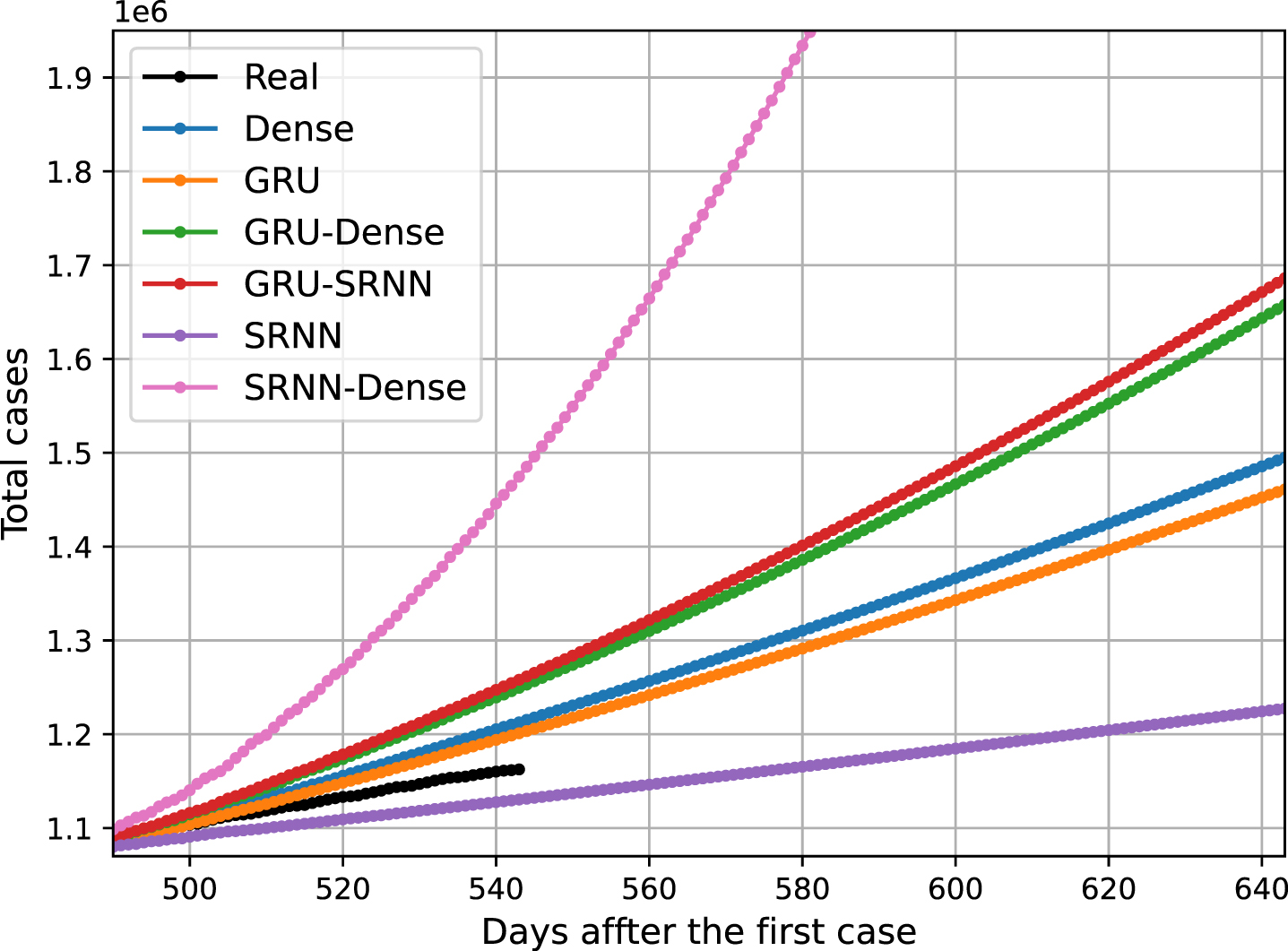
As can be seen in Figure 10 there is a big difference between forecasting results by changing the layer structure of the models. In this presentation, the best results were obtained using GRU and SRNN, as these values were closer to the real variation. The results presented in this image correspond to the comparison with the data set that was used for the model test.
5Conclusion
The proposed algorithm proved to be a promising technique for evaluating the increase in the number of cases and deaths confirmed by COVID-19. Considering that there was a mean R2 in the analysis of 0.9077 for the number of confirmed cases and 0.8861 for the number of deaths. Based on the forecast, it is possible to assess the capacity of the health system and to increase or relax the restriction measures.
According to the results presented in this article, it is possible to notice that the number of deaths follows the trend of the contamination curve, so reducing the slope of this curve is extremely necessary to consequently reduce the number of deaths. The trend presented in the results of this article shows that the vaccination programs applied so far are reducing the numbers of contamination. And government agencies, should consider these forecasts to determine if the restrictive measures are maintained or relaxed.
Comparing to other models the LSTM stacking shows a similar performance in terms of R2 an reduction of the error. The average and statistical analysis shows that the algorithm is stable and can be applied for forecast analysis in the COVID-19 spread.
The evaluation of the number of cases curve proves to be an excellent measure to reduce the number of emergency visits with high complexity, without the capacity of the health system. The combination of hybrid methods can be used to reduce variations in the algorithm that are not representative, such as those caused during weekends.
Fig. 10
Results for Each Layer Configuration for the Model.
Acknowledgments
The authors would like to thank the Coordination for the Improvement of Higher Education Personnel (CAPES), which awarded a PhD scholarship to one of the authors and the Institutional Program for Scientific Initiation Scholarships (PROBIC) at the Santa Catarina State University (UDESC), which granted scientific initiation scholarship to one of the authors.
This work was supported by national funds through the Fundação para a Ciêcia e a Tecnologia, I.P. (Portuguese Foundation for Science and Technology) by the project UIDB/05064/2020 (VALORIZA–Research Centre for Endogenous Resource Valorization) and it was partially supported by Fundação para a Ciência e a Tecnologia under Project UIDB/04111/2020, and ILIND–Instituto Lusófono de Investigação e Desenvolvimento, under project COFAC/ILIND/COPE LABS/3/2020.
References
[1] | Zhang S. , Diao M.Y. , Yu W. , Pei L. , Lin Z. and Chen D. , Estimationof the reproductive number of novel coronavirus (COVID-19) and theprobable outbreak size on the diamond princess cruise ship: Adata-driven analysis, International Journal of Infectious Diseases 93: ((2020) ), 201–204. |
[2] | Ribeiro M.H.D.M. , da Silva R.G. , Mariani V.C. and dos Santos Coelho L. , Short-term forecasting COVID-19 cumulative confirmed cases:Perspectives for Brazil. Chaos, Solitons & Fractals 135: (2020), 109853. |
[3] | Grasselli G. , Pesenti A. and Cecconi M. , Critical Care Utilizationfor the COVID-19 Outbreak in Lombardy, Italy: Early Experience and Forecast During an Emergency Response, JAMA 323: (16) ((2020) ), 1545–1546. |
[4] | Sohrabi C. , Alsafi Z. , O’Neill N. , Khan M. , Kerwan A. , Al-Jabir A. , Iosifidis C. and Agha R. , World health organization declares globalemergency: A review of the novel coronavirus (COVID-19), International Journal of Surgery 76: ((2020) ), 71–76. |
[5] | Petropoulos F. and Makridakis S. , Forecasting the novel coronavirus COVID-19, PLOS ONE 15: (3) ((2020) ), 1–8. |
[6] | Roosa K. , Lee Y. , Luo R. , Kirpich A. , Rothenberg R. , Hyman J.M. , Yan P. and Chowell G. , Real-time forecasts of the COVID-19 epidemic inchina from february 5th to february 24th, 2020, Infectious Disease Modelling 5: ((2020) ), 256–263. |
[7] | Pinto E.R. , Nepomuceno E.G. and Campanharo A.S. , Impact of networktopology on the spread of infectious diseases, TEMA 21: (1) ((2020) ), 95–115. |
[8] | Wynants L. , Van Calster B. , Bonten M.M.J. , Collins G.S. , Debray T.P.A. , De Vos M. , Haller M.C. , Heinze G. , Moons K.G.M. , Riley R.D. , Schuit E. , Smits L.J.M. , Snell K.I.E. , Steyerberg E.W. , Wallischand C. and Van Smeden M. , Prediction models for diagnosis and prognosis ofCOVID-19 infection: systematic review and critical appraisal, 369: ((2020) ), 1–11. |
[9] | Al-qaness M.A.A. , Ewees A.A. , Fan H. and Abd El Aziz M. , Optimization method for forecasting confirmed cases of covid-19 inchina, Journal of Clinical Medicine 9: (3) ((2020) ), 674. |
[10] | Sajadi M.M. , Habibzadeh P. , Vintzileos A. , Shokouhi S. , Miralles-Wilhelm F. and Amoroso A. , Temperature and latitude analysis to predict potential spread and seasonality for COVID-19, SSRN, (2020). |
[11] | Fanelli D. and Piazza F. , Analysis and forecast of COVID-19 spreading in china, italy and france, Cha., Sol. & Frac. 134: ((2020) ), 109761. |
[12] | Roosa K. , Lee Y. , Luo R. , Kirpich A. , Rothenberg R. , Hyman J.M. , Yan P. and Chowell G. , Short-term forecasts of the COVID-19 epidemic inguangdong and zhejiang, china: February 13-23, 2020. Journal ofClinical Medicine 9: (2) ((2020) ), 596. |
[13] | He S. , Tang S. and Rong L. , A discrete stochastic model of theCOVID-19 outbreak: Forecast and control, MathematicalBiosciences and Engineering 17: ((2020) ), 2792–2804. |
[14] | Stefenon S.F. , Branco N.W. , Nied A. , Bertol D.W. , Finardi E.C. , Sartori A. , Meyer L.H. and Grebogi R.B. , Analysis of trainingtechniques of ANN for classification of insulators in electricalpower systems, IET Generation Transmission & Distribution 14: (8) ((2020) ), 1591–1597. |
[15] | Stefenon S.F. , Silva M.C. , Bertol D.W. , Meyer L.H. and Nied A. , Fault diagnosis of insulators from ultrasound detection using neuralnetworks, Journal of Intelligent & Fuzzy Systems 37: (5) ((2019) ), 6655–6664. |
[16] | Stefenon S.F. , Freire R.Z. , Coelho L.S. , Meyer L.H. , Grebogi R.B. , Buratto W.G. and Nied A. , Electrical insulator fault forecastingbased on a wavelet neuro-fuzzy system, Energies 13: (2) ((2020) ), 484. |
[17] | Ribeiro M.H.D.M. and Coelho L.S. , Ensemble approach based onbagging, boosting and stacking for short-term prediction inagribusiness time series, Applied Soft Computing 86: (2020), 105837. |
[18] | Stefenon S.F. , Grebogi R.B. , Freire R.Z. , Nied A. and Meyer L.H. , Optimized ensemble extreme learning machine for classification ofelectrical insulators conditions, IEEE Transactions onIndustrial Electronics 67: (6) ((2020) ), 5170–5178. |
[19] | Li M.-W. , Geng J. , Hong W.-C. and Zhang L.-D. , Periodogramestimation based on lssvr-ccpso compensation for forecasting shipmotion, Nonlinear Dynamics 97: (4) ((2019) ), 2579–2594. |
[20] | Fan G.-F. , Wei X. , Li Y.-T. and Hong W.-C. , Forecasting electricityconsumption using a novel hybrid model, Sustainable Cities andSociety 61: ((2020) ), 102320. |
[21] | Hong W.-C. and Fan G.-F. , Hybrid empirical mode decomposition withsupport vector regression model for short term load forecasting, Energies 12: (6) ((2019) ), 1093. |
[22] | Zhang Z. and Hong W.-C. , Electric load forecasting by completeensemble empirical mode decomposition adaptive noise and supportvector regression with quantum-based dragonfly algorithm, Nonlinear Dynamics 98: (2) ((2019) ), 1107–1136. |
[23] | Fan G.-F. , Guo Y.-H. , Zheng J.-M. and Hong W.-C. , A generalize dregression model based on hybrid empirical mode decomposition andsupport vector regression with back propagation neural network formid-short-term load forecasting, Journal of Forecasting 39: (5) ((2020) ), 737–756. |
[24] | Fan G.-F. , Peng L.-L. , Hong W.-C. and Sun F. , Electric loadforecasting by the svr model with differential empirical modedecomposition and auto regression, Neurocomputing 173: (2016), 958–970. |
[25] | Fan G.-F. , Qing S. , Wang H. , Hong W.-C. and Li H.-J. , Support vectorregression model based on empirical mode decomposition and autoregression for electric load forecasting, Energies 6: (4) ((2013) ), 1887–1901. |
[26] | Maleki M. , Mahmoudi M.R. , Wraith D. and Pho K.-H. , Time seriesmodelling to forecast the confirmed and recovered cases of covid-19, Travel Medicine and Infectious Disease 37: ((2020) ), 101742. |
[27] | Li H. , Xu X.-L. , Dai D.-W. , Huang Z.-Y. , Ma Z. and Guan Y.-J. , Airpollution and temperature are associated with increased covid-19incidence: a time series study, International Journal ofInfectious Diseases 97: ((2020) ), 278–282. |
[28] | Qi H. , Xiao S. , Shi R. , Ward M.P. , Chen Y. , Tu W. , Su Q. , Wang W. , Wang X. and Zhang Z. , Covid-19 transmission in mainland china isassociated with temperature and humidity: a time-series analysis, Science of The Total Environment 728: ((2020) ), 138778. |
[29] | Zeroual A. , Harrou F. , Dairi A. and Sun Y. , Deep learning methodsfor forecasting covid-19 time-series data: A comparative study, Chaos, Solitons & Fractals 140: ((2020) ), 110121. |
[30] | Chimmula V.K.R. and Zhang L. , Time series forecasting of covid-19transmission in canada using lstm networks, Chaos, Solitons & Fractals 135: ((2020) ), 109864. |
[31] | Shastri S. , Singh K. , Kumar S. , Kour P. and Mansotra V. , Time seriesforecasting of covid-19 using deep learning models: India-usacomparative case study, Chaos, Solitons & Fractals 140: (2020), 110227. |
[32] | Wang P. , Zheng X. , Ai G. , Liu D. and Zhu B. , Time series predictionfor the epidemic trends of covid-19 using the improved lstm deeplearning method: Case studies in russia, peru and iran, Chaos,Solitons & Fractals 140: ((2020) ), 110214. |
[33] | Stefenon S.F. , Kasburg C. , Nied A. , Klaar A.C.R. , Ferreiraand F.C.S. and Branco N.W. , Hybrid deep learning for power generationforecasting in active solar trackers, IET Generation,Transmission & Distribution 14: (23) ((2020) ), 5667–5674. |
[34] | Xiao F. , Time series forecasting with stacked long short-term memory networks, arXiv preprint arXiv:2011.00697, (2020). |
[35] | Liang S. , Nguyen L. and Jin F. , A multi-variable stacked longshort term memory network for wind speed forecasting, In 2018 IEEE International Conference on Big Data (Big Data), pages 4561–4564. IEEE, ((2018) ). |
[36] | Xu Y. , Chhim L. , Zheng B. and Nojima Y. , Stacked deep learning structure with bidirectional long-short term memory for stock market prediction, In International Conference on Neural Computing for Advanced Applications, pages 47–460. Springer, ((2020) ). |
[37] | Bao W. , Yue J. and Rao. Y. , A deep learning framework for financialtime series using stacked autoencoders and long-short term memory, PloS one 12: (7) ((2017) ), e0180944. |
[38] | Song P.X. , Wang L. , Zhou Y. , He J. , Zhu B. , Wang F. , Tang L. and Eisenberg M. , An epidemiological forecast model and software assessing interventions on COVID-19 epidemic in china. (2020), 1–8. |
[39] | Li Q. , Feng W. and Quan Y.-H. , Trend and forecasting of the COVID-19outbreak in china, Jour. of Infect. 80: (4) ((2020) ), 469–496. |
[40] | Vankadari N. and Wilce J.A. , Emerging COVID-19 coronavirus: glycanshield and structure prediction of spike glycoprotein and itsinteraction with human cd26, Emerging Microbes & Infections 9: (1) ((2020) ), 601–604. |
[41] | Li L. , Yang Z. , Dang Z. , Meng C. , Huang J. , Meng H. , Wang D. , Chen G. , Zhang J. , Peng H. and Shao Y. , Propagation analysis and prediction of the COVID-19, Infectious Disease Modelling 5: ((2020) ), 282–292. |
[42] | SC Controladoria Geral do Estado /Diário Oficial do Estado de Santa Catarina. Medida provisória n° 227 de 02 de abril de 2020, (2020). |
[43] | SC Governo do Estado de Santa Catarina. Enfrentamento ao COVID-19, (2020). |
[44] | Catarina N.D.S. , Plantão coronavírus: COVID-19 em Santa Catarina, (2020). |
[45] | Chen A. , Wang F. , Liu W. , Chang S. , Wang H. , He J. and Huang Q. , Multi-information fusion neural networks for arrhythmia automaticdetection, Computer Methods and Programs in Biomedicine 193: ((2020) ), 105479. |
[46] | Yildirim O. , Baloglu U.B. , Tan R.-S. , Ciaccio E.J. and Acharya U.R. , A new approach for arrhythmia classification using deep codedfeatures and lstm networks, Computer Methods and Programs in Biomedicine 176: ((2019) ), 121–133. |
[47] | Stefenon S.F. , Freire R.Z. , Meyer L.H. , Corso M.P. , Sartori A. , Nied A. , Klaar A.C.R. and Yow K.-C. , Fault detection in insulatorsbased on ultrasonic signal processing using a hybrid deep learningtechnique, IET Science, Measurement & Technology 14: (10) ((2020) ), 953–961. |
[48] | Nguyen X.A. , Ljuhar D. , Pacilli M. , Nataraja Ra M. and Chauhan S. , Surgical skill levels: Classification and analysis using deep neuralnetwork model and motion signals, Computer Methods and Programsin Biomedicine 177: ((2019) ), 1–8. |
[49] | Kasburg C. and Stefenon S.F. , Deep learning for photovoltaicgeneration forecast in active solar trackers, IEEE LatinAmerica Transactions 17: (12) ((2019) ), 2013–2019. |
[50] | Stefenon S.F. , Ribeiro M.H.D.M. , Nied A. , Mariani V.C. , Coelho L.S. , Leithardt V.R.Q. , Silva L.A. and Seman L.O. , Hybrid wavelet stackingensemble model for insulators contamination forecasting, IEEE Access 9: ((2021) ), 66387–66397. |
[51] | Stefenon S.F. , Seman L.O. , Furtado Neto C.S. , Nied A. , Seganfredo D.M. , da Luz F.G. , Sabino P.H. , González J.T. and Leithardt V.R.Q. , Electric field evaluation using the finite element methodand proxy models for the design of stator slots in a permanentmagnet synchronous motor, Electronics 9: (11) ((2020) ), 1975. |
[52] | Melinte D.O. and Vladareanu L. , Facial expressions recognition forhuman-robot interaction using deep convolutional neural networkswith rectified adam optimizer, Sensors 20: (8) ((2020) ), 2393. |
[53] | dos Santos G.H. , Seman L.O. , Bezerra E.A. , Leithardt V.R.Q. , Mendes A.S. and Stefenon S.F. , Static attitude determination usingconvolutional neural networks, Sensors 21: (19) ((2021) ). |
[54] | Halgamuge M.N. , Daminda E. and Nirmalathas A. , Best optimizerselection for predicting bushfire occurrences using deep learning, Natural Hazards 103: ((2020) ), 845–860. |
[55] | Wibowo A. , Wiryawan P.W. and Nuqoyati N.I. , Optimization of neuralnetwork for cancer microrna biomarkers classification, In, Journal of Physics: Conference Series 1217: 012124. IOP Publishing, ((2019) ). |
[56] | Stefenon S.F. , Steinheuser D.F. , Silva M.P. , Ferreira F.C.S. , Klaar A.C.R. , Souza K.E. , Godinho Júnior A. , Venção A.T. , Branco R. and Yamaguchi C.K. , Application of active methodologies inengineering education through the integrative evaluation at theuniversidade do planalto catarinense, brazil, Interciencia 44: (7) ((2019) ), 408–413. |
[57] | Stefenon S.F. , Ribeiro M.H.D.M. , Nied A. , Mariani V.C. , Coelho L.S. , Rocha D.F.M. , Grebogi R.B. and Ruano A.E.B. , Wavelet group method ofdata handling for fault prediction in electrical power insulators, International Journal of Electrical Power & Energy Systems 123: ((2020) ), 106269. |
[58] | Stefenon S.F. , Kasburg C. , Freire R.Z. , Ferreira F.C.S. , Bertoland D.W. and Nied A. , Photovoltaic power forecasting using waveletneuro-fuzzy for active solar trackers, Journal of Intelligent& Fuzzy Systems 40: (1) ((2021) ), 1083–1096. |
[59] | He J. and Wang Y. , Blood glucose concentration prediction based onkernel canonical correlation analysis with particle swarmoptimization and error compensation, Computer Methods and Programs in Biomedicine 196: ((2020) ), 105574. |
[60] | Huang J.-C. , Tsai Y.-C. , Wu P.-Y. , Lien Y.-H. , Chien C.-Y. , Kuo C.-F. , Hung J.-F. , Chen S.-C. and Kuo C.-H. , Predictive modeling of blood pressure during hemodialysis: a comparison of linear model,random forest, support vector regression, xgboost, lasso regressionand ensemble method, Computer Methods and Programs in Biomedicine 195: ((2020) ), 105536. |
[61] | Stefenon S.F. , Ribeiro M.H.D.M. , Nied A. , Yow K.-C. , Mariani V.C. , Coelho L.S. and Seman L.O. , Time series forecasting using ensemblelearning methods for emergency prevention in hydroelectric powerplants with dam, Electric Power Systems Research 202: (2022), 107584. |
[62] | Ribeiro M.H.D.M. , Stefenon S.F. , de Lima J.D. , Nied A. , Marianiand V.C. and Coelho L.S. , Electricity price forecasting based onself-adaptive decomposition and heterogeneous ensemble learning, Energies 13: (19) ((2020) ), 5190. |
[63] | Sopelsa Neto N.F. , Stefenon S.F. , Meyer L.H. , Bruns R. , Nied A. , Seman L.O. , Gonzalez G.V. , Leithardt V.R.Q. and Yow K.-C. , A studyof multilayer perceptron networks applied to classification ofceramic insulators using ultrasound, Applied Sciences 11: (4) ((2021) ), 1592. |
[64] | Erdenebayar U. , Kim Y.J. , Park J.-U. , Joo E.Y. and Lee K.-J. , Deeplearning approaches for automatic detection of sleep apnea eventsfrom an electrocardiogram, Computer Methods and Programs in Biomedicine 180: ((2019) ), 105001. |


