Evaluation of missile electromagnetic launch system based on effectiveness

Li, Qiaoyang; Chen, Guiming; Li, Ziqi; Zhang, Yi; Xu, Lingliang

doi:10.3233/JIFS-210353

Evaluation of missile electromagnetic launch system based on effectiveness

Article type: Research Article

Authors: Li, Qiaoyang^{; *} | Chen, Guiming | Li, Ziqi | Zhang, Yi | Xu, Lingliang

Affiliations: Xi’an Research Institute of High-Tech, Xi’an, China

Correspondence: [*] Corresponding author. Qiaoyang Li, Xi’an Research Institute of High-Tech, Xi’an, China. E-mail: liqiaoyang2019@163.com.

Keywords: MEMLS, Grey relation analysis (GRA), Principal component analysis (PCA), Least square support vector machine (LSSVM), Data Envelopment Analysis (DEA)

DOI: 10.3233/JIFS-210353

Journal: Journal of Intelligent & Fuzzy Systems, vol. 41, no. 6, pp. 6517-6526, 2021

Published: 16 December 2021

Get PDF

Abstract

To solve the problems of strong infrared radiation, poor continuous combat capability of the system, serious ablation of the launching device, and environmental pollution of the existing missile launching system, electromagnetic launch system (EMLS) has been studied for missile launch system. Combining the situation that the current research on missile electromagnetic launch system (MEMLS) mainly focuses on the key technical points and the deficiencies in the previous research on MEMLS, this paper establishes an effectiveness prediction model based on GRA-PCA-LSSVM, and discusses the investment efficiency of the system based on DEA. The experimental results prove that the established model is reasonable, effective and superior, and provides a reference for the further improvement and development of MEMLS.

1Introduction

Electromagnetic launch system (EMLS) is a launching technology that uses electromagnetic energy to convert it into payload kinetic energy [1]. EMLS can convert electrical energy into the kinetic energy required by the load in a short time, and push objects to reach a certain speed quickly [2]. Since it can effectively solve the problems of strong infrared radiation, poor continuous combat capability of the system, serious ablation of the launcher, and environmental pollution of the existing system, missile electromagnetic launch system (MEMLS) is a current research hotspot.

The current research on MEMLS concentrates on technical points such as pulse energy storage power supply, pulse power discharge, motor control, etc. There are few studies on the whole system evaluation. The author has studied the effectiveness evaluation method of MEMLS and proposed a new evaluation model for the two-level indicators of the system [3]. However, the system has many evaluation indicators and the model is quite complex, so the effectiveness value of the design scheme cannot be calculated quickly, and the investment efficiency of the design scheme is not discussed.

Aiming at the problem of too many evaluation indexes, Wang used gray correlation analysis (GRA) and support vector machine (SVM) to study and optimize the performance of asphalt pavement [4]; Yu proposed an improved principal component analysis (PCA) model to study the fault detection of nuclear power station sensors [5]. For the study of prediction model, Chung used multi-channel convolutional neural network optimized by genetic algorithm to predict the stock market [6]; Stoichev used multiple regression model to study the pollution of metals and quasi metals in surface sediments [7]; Liu used SVM model optimized by particle swarm optimization to analyze and predict PM2.5 [8]. To solve the problem of investment efficiency, Yeung used data envelopment analysis (DEA) to study the efficiency of Brazilian courts [9]; Yang used DEA to evaluate the efficiency of China’s industrial waste gas treatment [10].

Existing research models only solve part of the problems, and there are few in the field of MEMLS. This paper evaluates MEMLS based on effectiveness, focusing on the rapid calculation of effectiveness model and system investment efficiency. The main innovations are as follows.

(1) From the perspective of the system, this paper conducts further research on the effectiveness calculation model of MEMLS, which makes up for the lack of most research focusing on specific technologies.

(2) This paper establishes the effectiveness calculation model of GRA-PCA-LSSVM, which can quickly calculate the effectiveness value of MEMLS.

(3) This paper uses the DEA model to study the investment efficiency of MEMLS, and proposes suggestions for improvement of the design scheme.

(4) This paper supplements the deficiencies of the previous research, which is innovative and practical.

The main structure of this paper is as follows: Section 1 introduces the basic concepts and advantages of EMLS and MEMLS, and points out the status and shortcomings of the current research of MEMLS; Section 2 establishes a model for fast calculation of effectiveness and investment efficiency of MEMLS; Section 3 combines the existing sample data to apply and verify the model, which proves the effectiveness of the model and methods; Section 4 summarizes this paper.

2System evaluation model based on effectiveness

This section mainly introduces the model established in this paper for MEMLS evaluation. The steps and methods of model establishment are shown in Fig. 1.

Fig. 1

Evaluation model based on effectiveness.

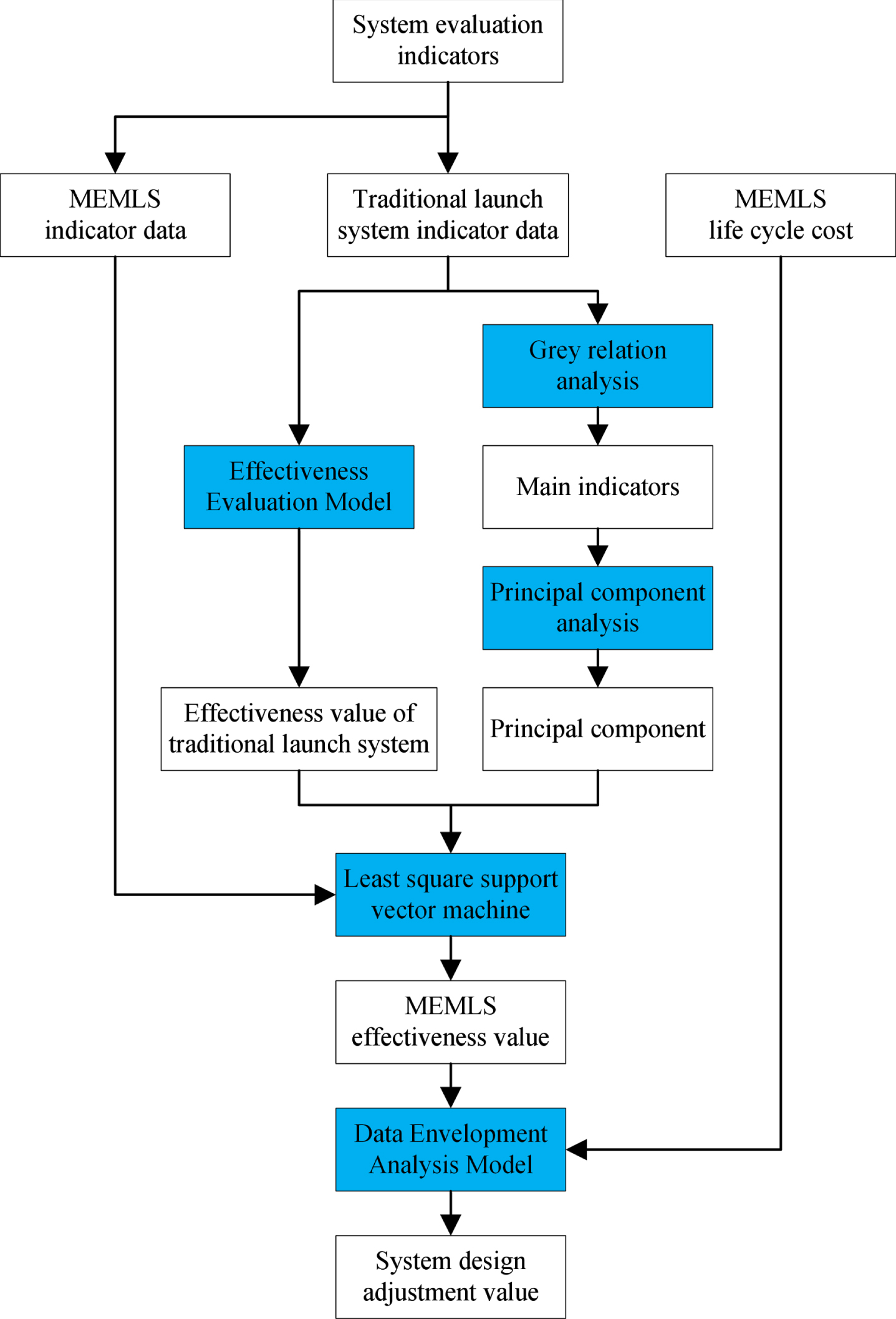
The effectiveness evaluation model in Fig. 1 has been studied in the early stage [3], and is used directly as a model here.

2.1Effectiveness calculation model based on GRA-PCA-LSSVM

To solve the problem that the original effectiveness evaluation model is too complicated, firstly establish a fast calculation model of effectiveness based on GRA-PCA-LSSVM, which is convenient to directly obtain the effectiveness value from the design scheme of MEMLS.

2.1.1GRA

When evaluating the system, there are too many original evaluation indicators, which will lead to the redundancy of information and the complexity of the process. Therefore, it is necessary to select the main indicators. Grey system theory was founded in 1982 by Professor Deng Julong of China. It is a system control theory about the incomplete or uncertain internal system [11]. GRA is a multi-factor statistical analysis method in grey system theory, which judges the correlation degree according to the similarity degree of the changing trends between factors. Because of its simple calculation and low sample requirements, GRA has been widely used in industry, materials, and agriculture [12–14]. The steps of GRA are as follows.

Step 1: Determine the parent sequence and subsequence in the system. The parent sequence is a sequence that reflects the characteristics of the system’s behavior, and the subsequence is a sequence that affects the characteristics of the system’s behavior.

Step 2: Dimensionless processing of the parent sequence and subsequence. In the analysis process, different dimensions may lead to errors in the results. Generally, the sequence is processed by the averaging method to remove dimensions.

Step 3: Calculate the correlation coefficient of the factors corresponding to the sub-sequence and the parent sequence, as shown in formula (1).

(1)

ξ(x0(k),xi(k))=minimink|x0(k)-xi(k)|+ρmaximaxk|x0(k)-xi(k)||x0(k)-xi(k)|+ρmaximaxk|x0(k)-xi(k)|,{i=1,2,⋯,mk=1,2,⋯,n

In the formula: m is the number of subsequences; n is the number of samples; x₀ (k) is the k-th sample value of the parent sequence after dimensionless processing; x_i (k) is the k-th sample of the i-th subsequence after dimensionless processing Value; ρ is the resolution coefficient, reflecting the size of the resolution, usually 0.5.

Step 4: Calculate the degree of relevance and sort to obtain the degree of relevance of each sub-sequence to the parent sequence, as shown in formula (2).

(2)

ri=1n∑k=1nξ(x0(k),xi(k)),i=1,2,⋯,m

2.1.2PCA

PCA is a multivariate statistical analysis method that converts multiple interrelated indicators into a few comprehensive indicators. In the research of multiple indicators, Since there is often a certain correlation between the indicators, the data will overlap with information, which is more complicated for high-dimensional research. PCA adopts the method of dimensionality reduction, and uses a small number of comprehensive factors to express all the original indicators, and requires that the original indicator information is reflected as much as possible, and the factors are not related to each other. PCA has been widely used in environmental science, agriculture and industry [15–17]. The steps of PCA are as follows.

Step 1: Standardize the original data to eliminate the influence of different dimensions and orders of magnitude on the analysis results.

Step 2: Perform correlation analysis on the processed sample matrix to obtain the correlation coefficient matrix, and determine whether PCA can be performed.

Step 3: From the correlation coefficient matrix, the eigenvalue and variance are calculated by the Jacobian method, and the principal component variance contribution rate and cumulative contribution rate are calculated.

Step 4: Select the principal component according to the specific requirements of the eigenvalue or the cumulative contribution rate of the principal component to complete the PCA. The general mathematical model of PCA results is shown in formula (3).

(3)

Z1=a11X1+a12X2+⋯+a1nXnZ2=a21X1+a22X2+⋯+a2nXn⋮Zl=al1X1+al2X2+⋯+alnXn

In the formula: Z_l is the main component; X_n is the normalized raw data; a_ij is the main component coefficient.

2.1.3LSSVM

Least Square Support Vector Machine (LSSVM) is an extension of SVM. LSSVM takes the quadratic loss function as the empirical risk, and replaces the inequality constraints with equality constraints, transforming the training of the model into the calculation of linear equations, reducing the computational complexity [18]. Because of its superiority, LSSVM is widely used in meteorology, materials science, industry and other fields [19–21]. The establishment process of the LSSVM model is as follows.

Suppose that the number of samples is n, x_i is the m-dimensional input vector, and y_i is the output vector. Construct the optimal linear regression function as formula (4).

(4)

f(x)=ωTφ(x)+b

In the formula: ω is the weight vector; b is the offset; φ (x) is the nonlinear mapping.

According to the principle of structural risk minimization, the objective function can be expressed as formula (5).

(5)

min12ωTω+λ2∑i=inei2

Where: λ is the regularization parameter; e_i is the prediction error vector of the training set.

The constraint condition is formula (6).

(6)

yi=ωTφ(xi)+b+ei

The Lagrangian function is used to transform the problem into the dual space, as in formula (7).

(7)

L=12ωTω+λ2∑i=inei2-∑i=1nαi[ωTφ(xi)+b+ei-yi]

In the formula: α_i is the Lagrange multiplier. According to the KKT condition, the formula (8) can be obtained.

(8)

{ω=∑i=1nαiφ(xi)∑i=1nαi=0αi=λeiωTφ(xi)+b+ei-yi

Eliminate ω and e_i in formula (8) to obtain formula (9).

(9)

[01⋯11K(x1,x1)+1c⋯K(x1,x1)⋮⋮⋮1K(xn,xn)⋯K(xn,xn)+1c][bα1⋮αn]=[0y1⋮yn]

In the formula: K (x_i, x_j) =< φ (x_i) , φ (x_j) > is the kernel function. Generally take the radial basis kernel function as equation (10).

(10)

K(xi,xj)=exp(-∥xi-xj∥22μ2)

In the formula: μ is the nuclear parameter.

Finally, the prediction model of LSSVM is

(11)

y(x)=∑i=1nαiK(xi,xj)+b

2.2Evaluation of system investment efficiency based on DEA model

The DEA method is a non-parametric method used to evaluate the relative effectiveness of decision-making units (DMUs) with the same type of multiple inputs and multiple outputs. At present, DEA research is relatively mature and widely used in economics, sociology and industry [22–24].

2.2.1Overall effectiveness evaluation model (CCR)

Suppose there are a total of s DMUs, each DMU has p inputs and q outputs, x_k = (x_1k, x_2k, ⋯ , x_pk) ^T represents the input vector of the k-th DMU, y_k = (x_1k, x_2k, ⋯ , x_qk) ^T represents the output vector of the k-th DMU, and x₀ and y₀ represent the input and output vectors of the DMU₀. From the literature [25], the BCC model is:

(12)

{minθs.t.∑k=1sλkxk+s-=θx0∑k=1sλkxk-s+=y0s-⩾0,s+⩾0

In the formula: s^- and s⁺ are slack variables; λ_k is a general variable.

To simplify the calculation, the non-Archimedean infinitesimal quantity is introduced, then the formula (12) becomes

(13)

{min[θ-ɛ(eˆTs-+eˆTs+)]s.t.∑k=1sλkxk+s-=θx0∑k=1sλkxk-s+=y0s-⩾0,s+⩾0

If the optimal solutions of the model are λ^*, s^-*, s^+* and θ^*, then there are the following conclusions.

(1) If θ^*< 1, then DMU₀ is not DEA effective. This scheme neither meets the requirements of the best technical efficiency nor the constant return of scale.

(2) If θ^*= 1, and at least one of s^-* and s^+* is not 0, then DMU₀ is weak DEA effective, that is, it is not both technically effective and scale effective.

(3) If θ^*= 1 and s^-*= s^+*= 0, then DMU₀ is DEA effective, that is, both technical efficiency and scale efficiency are satisfied.

2.2.2Technical effectiveness evaluation model (BCC)

The BCC model is used to evaluate the relative technical effectiveness. Similarly, the calculation model can be obtained as follows.

(14)

{max[θ-ɛ(eˆTs-+eˆTs+)]=Vs.t.∑k=1sλkxk+s-=θx0∑k=1sλk=1λk⩾0,s-⩾0,s+⩾0

If the optimal solutions of the model are λ^*, s^-*, s^+* and θ^*, when θ⁰= 1 and s^-0= s⁺⁰= 0, DMU₀ is technically effective, otherwise it is not technically effective.

2.2.3Scale effectiveness evaluation model

Scale validity refers to verifying whether the DMU is at the optimal scale level, and it can be judged whether it is in a state of increasing, constant or decreasing scale. The scale efficiency of DMU is represented by Q=θV . Calculate K=∑k=1sλk . When K = 1, the scale efficiency is unchanged; when K < 1, the scale efficiency increases; when K > 1, the scale efficiency decreases.

3Evaluation of MEMLS based on effectiveness

3.1Effectiveness calculation based on GRA-PCA-LSSVM

From the author’s previous research [3], the effectiveness evaluation indicators of MEMLS can be obtained as shown in Table 1. From the related research of the subject, 64 sets of sample data for traditional launch methods can be obtained as shown in Table 2. Each set of data includes 18 evaluation indicators and the effectiveness value.

Table 1

MEMLS effectiveness evaluation indicators table

Target layer	First-level indicator layer	Second-level indicator layer
Effectiveness evaluation of MEMLS	Launch capability U₁	Thrust control accuracy U₁₁
		Robustness during launch U₁₂
		Maximum thrust U₁₃
		Acceleration time U₁₄
		Initial ejection velocity U₁₅
	Confrontation capability U₂	Infrared radiation intensity U₂₁
		Electromagnetic anti-interference ability U₂₂
		Electromagnetic compatibility of own system U₂₃
		Initial anti-interception rate U₂₄
	State loss U₃	Energy utilization rate U₃₁
		Ablation degree of the launcher U₃₂
		Environmental pollution degree U₃₃
		Spare parts replacement rate U₃₄
	Expanding ability U₄	Ejection power unit weight U₄₁
		Launcher weight U₄₂
		Space-ratio performance U₄₃
		Continuous combat capability U₄₄
		Universality of launch system U₄₅

Table 2

Effectiveness and indicators data of missile launch system

No.	Indicators
	U₁₁	U₁₂	U₁₃	U₁₄	U₁₅	U₂₁	U₂₂	U₂₃	U₂₄	U₃₁	U₃₂	U₃₃	U₃₄	U₄₁	U₄₂	U₄₃	U₄₄	U₄₅	E
1	0.9	0.6	250	15	35	25	0.9	0.5	0.7	0.8	0.9	0.4	0.6	350	6	0.4	0.6	0.2	0.6371
2	0.7	0.6	250	10	35	25	0.9	0.5	0.6	0.7	0.9	0.4	0.3	350	3	0.6	0.4	0.2	0.6239
3	0.5	0.6	250	10	35	25	0.9	0.5	0.6	0.5	0.9	0.4	0.3	350	3	0.3	0.4	0.2	0.5851
4	0.5	0.6	250	20	35	25	0.9	0.7	0.7	0.8	0.9	0.8	0.7	350	3	0.3	0.5	0.2	0.6669
5	0.5	0.6	250	10	40	25	0.9	0.7	0.8	0.5	0.9	0.4	0.3	350	6	0.3	0.7	0.2	0.5997
6	0.7	0.9	250	20	35	25	0.9	0.4	0.7	0.9	0.9	0.4	0.6	350	6	0.3	0.5	0.2	0.6152
7	0.9	0.5	250	20	35	25	0.9	0.4	0.8	0.9	0.7	0.8	0.6	350	3	0.3	0.5	0.2	0.6534
8	0.9	0.5	250	10	35	25	0.9	0.4	0.6	0.9	0.4	0.4	0.3	350	3	0.5	0.7	0.2	0.6059
9	0.5	0.9	250	20	37	25	0.9	0.4	0.6	0.9	0.8	0.4	0.3	350	7	0.4	0.5	0.5	0.5896
10	0.9	0.5	250	10	35	25	0.9	0.4	0.6	0.9	0.7	0.4	0.6	350	7	0.5	0.5	0.5	0.6361
11	0.5	0.5	250	15	40	25	0.6	0.4	0.6	0.9	0.4	0.6	0.6	350	7	0.6	0.5	0.2	0.5514
12	0.9	0.5	250	10	37	25	0.5	0.4	0.8	0.9	0.4	0.4	0.7	400	7	0.4	0.5	0.5	0.6015
13	0.9	0.5	250	20	35	25	0.6	0.4	0.7	0.9	0.6	0.6	0.3	300	7	0.6	0.5	0.5	0.5741
14	0.9	0.7	250	10	35	25	0.6	0.7	0.6	0.9	0.6	0.8	0.3	500	7	0.4	0.5	0.2	0.6240
15	0.7	0.5	250	20	37	25	0.6	0.5	0.6	0.9	0.6	0.8	0.3	300	7	0.4	0.7	0.7	0.6026
. . .	. . .	. . .	. . .	. . .	. . .	. . .	. . .	. . .	. . .	. . .	. . .	. . .	. . .	. . .	. . .	. . .	. . .	. . .	. . .
61	0.6	0.9	150	10	39	10	0.5	0.9	0.6	0.7	0.4	0.9	0.3	500	9	0.8	0.5	0.2	0.6366
62	0.6	0.9	150	10	39	16	0.5	0.9	0.7	0.5	0.4	0.9	0.7	300	9	0.8	0.5	0.7	0.6847
63	0.6	0.5	150	10	39	10	0.7	0.9	0.7	0.7	0.8	0.9	0.3	480	9	0.8	0.5	0.2	0.6637
64	0.6	0.7	150	20	39	16	0.6	0.9	0.6	0.5	0.4	0.9	0.6	480	9	0.8	0.5	0.2	0.5855

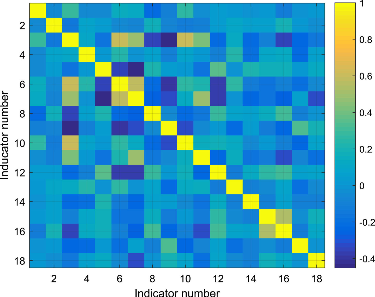
Due to the large number of indicators and the complexity of the evaluation method in literature [3], it needs to be simplified. First, perform a statistical description of the sample data as shown in Table 3, and make an indicator correlation strength diagram as shown in Fig. 2. The horizontal and vertical coordinates of Fig. 2 are indicator numbers, the color indicates the intensity of correlation, and the right side is the intensity and color contrast scale. It can be seen from Fig. 2 that there is a certain correlation between the indicators, so it can be considered to select and reduce the dimensionality of the indicators through GRA-PCA.

Table 3

Mathematical statistics of the original data of MEMLS

Evaluation Indicator	Minimum	Maximum	Average	Standard deviation
U₁₁	0.50	0.90	0.6375	0.15379
U₁₂	0.50	0.90	0.6547	0.16323
U₁₃	150.00	250.00	195.4688	41.01605
U₁₄	10.00	20.00	15.3906	4.07321
U₁₅	35.00	40.00	37.0937	1.96573
U₂₁	10.00	25.00	18.7812	6.62719
U₂₂	0.40	0.90	0.6047	0.15779
U₂₃	0.40	0.90	0.6156	0.16351
U₂₄	0.60	0.90	0.7625	0.12536
U₃₁	0.50	0.90	0.6844	0.16057
U₃₂	0.40	0.90	0.5859	0.17716
U₃₃	0.40	0.90	0.6141	0.18845
U₃₄	0.30	0.80	0.4953	0.18724
U₄₁	300.00	500.00	380.9375	72.93656
U₄₂	3.00	9.00	5.8125	2.30166
U₄₃	0.30	0.80	0.5297	0.15704
U₄₄	0.40	0.90	0.5750	0.17817
U₄₅	0.20	0.70	0.4000	0.21381

Fig. 2

Indicator correlation strength diagram.

According to formulas (1)-(2), the correlation between each indicator and effectiveness is calculated, as shown in Table 4. The main indicators are selected with the degree of correlation > 0.7, that is, U₁₁, U₁₂, U₁₃, U₁₅, U₂₂, U₂₄, U₃₁ and U₄₁.

Table 4

Correlation degree of each indicator and effectiveness

Indicator	U₁₁	U₁₂	U₁₃	U₁₄	U₁₅	U₂₁	U₂₂	U₂₃	U₂₄
correlation	0.7165	0.7155	0.7206	0.6571	0.8688	0.5897	0.7112	0.6775	0.7616
Indicator	U₃₁	U₃₂	U₃₃	U₃₄	U₄₁	U₄₂	U₄₃	U₄₄	U₄₅
correlation	0.7348	0.6675	0.6729	0.5925	0.7464	0.5944	0.6618	0.6647	0.4983

After GRA, in order to further reduce the number of indicators and simplify the model, PCA was performed on the selected 8 indicators. According to Section 2.1.2, the correlation coefficient matrix is calculated as shown in Table 5, and the variance contribution rate of each principal component is calculated as shown in Table 6.

Table 5

Correlation coefficient matrix of PCA

		U₁₁	U₁₂	U₁₃	U₁₅	U₂₂	U₂₄	U₃₁	U₄₁
Correlation coefficient	U₁₁	1.000	–0.051	0.284	–0.054	0.137	–0.091	0.268	–0.020
	U₁₂	–0.051	1.000	–0.138	0.038	–0.084	–0.069	–0.112	0.056
	U₁₃	0.284	–0.138	1.000	–0.158	0.494	–0.444	0.604	–0.207
	U₁₅	–0.054	0.038	–0.158	1.000	–0.452	0.047	0.015	0.208
	U₂₂	0.137	–0.084	0.494	–0.452	1.000	–0.328	0.122	–0.235
	U₂₄	–0.091	–0.069	–0.444	0.047	–0.328	1.000	–0.329	0.033
	U₃₁	0.268	–0.112	0.604	0.015	0.122	–0.329	1.000	–0.061
	U₄₁	–0.020	0.056	–0.207	0.208	–0.235	0.033	–0.061	1.000

Table 6

Variance contribution rate of PCA

Principal component	Variance	Contribution rate / %	Cumulative contribution rate / %
1	2.472	30.899	30.899
2	1.360	17.006	47.905
3	1.067	13.336	61.241
4	0.894	11.171	72.411
5	0.850	10.622	83.034
6	0.610	7.627	90.660
7	0.480	5.999	96.659
8	0.267	3.341	100.000

Here, the cumulative contribution rate > 90%is taken as the target, so 6 principal components need to be extracted, and the corresponding coefficients of 6 principal components and 8 main indicators can be obtained as shown in Table 7.

Table 7

Principal component coefficient

Indicators	Principal component
	1	2	3	4	5	6
U₁₁	0.411	0.285	–0.250	0.772	0.121	–0.262
U₁₂	–0.179	0.024	0.848	0.314	0.325	0.168
U₁₃	0.864	0.182	–0.016	–0.102	0.029	0.102
U₁₅	–0.387	0.704	–0.027	–0.255	0.237	–0.356
U₂₂	0.698	–0.449	0.128	0.029	–0.244	–0.185
U₂₄	–0.597	–0.234	–0.483	0.264	0.163	0.344
U₃₁	0.645	0.521	–0.105	–0.099	0.133	0.453
U₄₁	–0.340	0.471	0.153	0.206	–0.754	0.136

According to Table 7 and formula (3), the calculation expression of the principal components can be obtained as follows.

In the formula: U₁₁, U₁₂, U₁₃, U₁₅, U₂₂, U₂₄, U₃₁ and U₄₁ represent normalized data values.

According to formula (15), Table 2 can be transformed into Table 8.

Z1=0.411U11-0.179U12+0.864U13-0.387U15+0.698U22-0.597U24+0.645U31-0.340U41Z2=0.285U11+0.024U12+0.182U13+0.704U15-0.449U22-0.234U24+0.521U31+0.471U41Z3=-0.250U11+0.848U12-0.016U13-0.027U15+0.128U22-0.483U24-0.105U31+0.153U41Z4=0.772U11+0.314U12-0.102U13-0.225U15+0.029U22+0.264U24-0.099U31+0.206U41Z5=0.121U11+0.325U12+0.029U13+0.237U15-0.244U22+0.163U24+0.133U31-0.754U41

(15)

Z6=-0.262U11+0.168U12+0.102U13-0.356U15-0.185U22+0.344U24+0.453U31+0.136U41

Table 8

Effectiveness and principal components data of MEMLS

No.	Principal component						E
	Z₁	Z₂	Z₃	Z₄	Z₅	Z₆
1	2.8840	–0.4945	–0.3521	1.1770	0.2571	–0.3028	0.6371
2	2.5919	–0.9309	0.3985	–0.0433	0.6588	–0.5791	0.6239
3	1.7415	–1.8053	0.8395	–0.9752	1.0095	–0.8654	0.5851
4	2.2044	–1.1306	0.2770	–0.9479	0.5988	0.5689	0.6669
5	0.5092	–0.5886	0.0280	–1.2162	0.0737	–1.3226	0.5997
6	2.5900	–0.4967	1.4089	0.6603	–0.3102	0.8904	0.6152
7	2.9061	–0.3887	–1.2914	1.1311	0.2423	0.2773	0.6534
8	3.5122	–0.0692	–0.5458	0.6849	0.5242	–0.4248	0.6059
9	2.3028	–0.0406	2.0698	–0.9002	–0.2601	0.5115	0.5896
10	3.5122	–0.0692	–0.5458	0.6849	0.5242	–0.4248	0.6361
. . .	. . .	. . .	. . .	. . .	. . .	. . .	. . .
61	–1.1979	1.6010	2.0404	0.1202	0.6631	–0.2537	0.6366
62	–1.4189	–0.2224	1.3889	–0.1226	–1.5413	–1.1040	0.6847
63	–0.5998	0.7927	–0.2291	–0.4926	1.4972	–0.7784	0.6637
64	–1.2283	0.6651	1.1983	–0.1970	1.2183	–1.4377	0.5855

The principal components are used as input, and the effectiveness is used as output, and regression fitting is performed. According to formulas (4)-(11), model training is performed and compared with PSOSVM and BP neural network algorithms. Select 85%of the samples as the training set and 15%of the samples as the test set. The fitting effect of the training set is shown in Fig. 3 and the fitting effect of the test set is shown in Fig. 4.

Fig. 3

Fitting diagram of the training set of effectiveness value.

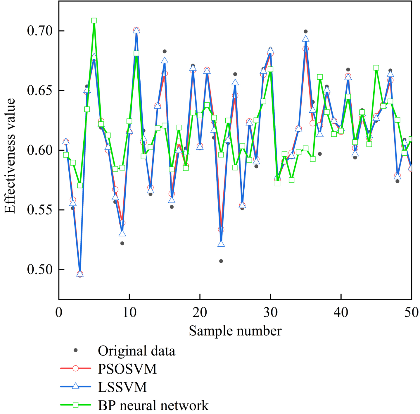
Fig. 4

Fitting diagram of the test set of effectiveness value.

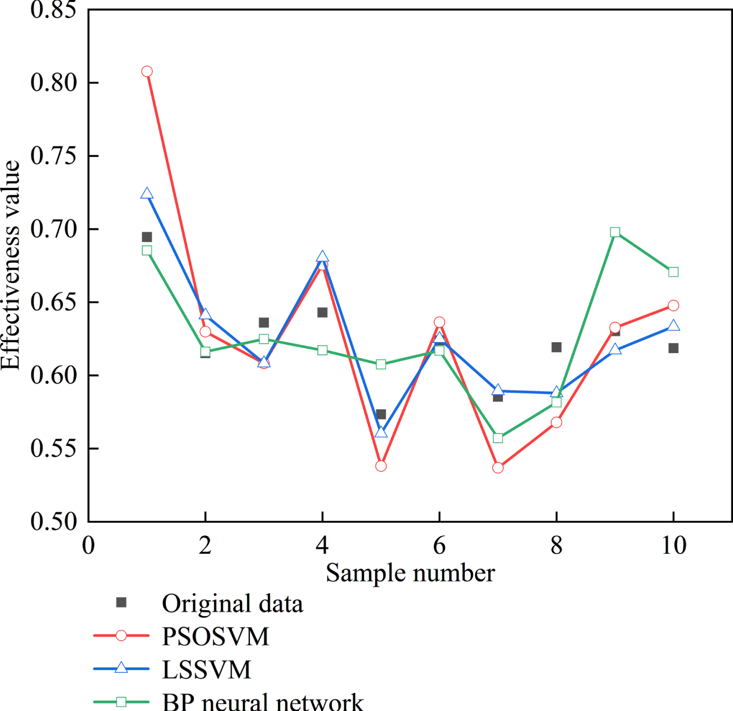
It can be intuitively obtained from Fig. 3 and Fig. 4 that the effect of the LSSVM model is better than that of PSOSVM and BP neural network. In order to get a specific comparison, calculate the mean square error (MSE) of the training set and the test set, as shown in Table 9.

Table 9

Performance comparison

Performance	PSOSVM	LSSVM	BP neural netwok
Optimal Parameters	Maxgen = 300	Gam = 400	Hidden layer = 10
	Sizepop = 50	Sig2 = 5	Learning rate = 0.01
			MaxEpochs = 5000
Train-MSE	7.8520e-05	2.0358e-05	0.0014
Test-MSE	0.0022	5.2525e-04	0.0012
Time	66.009s	0.535s	1.710s

It can be seen from Table 9 that the MSE of the training and test sets using the LSSVM model is the smallest, and the running time is the fastest, which can be further applied to the MEMLS design.

Each indicator value of the MEMLS design scheme is obtained from the research of the subject, and the effectiveness value is obtained through the pre-trained LSSVM model, as shown in Table 10.

Table 10

Design indicators and effectiveness values of MEMLS

Scheme Number	U₁₁	U₁₂	U₁₃	U₁₅	U₂₂	U₂₄	U₃₁	U₄₁	E
1	0.9	0.8	200	37	0.9	0.8	0.8	350	0.6779
2	0.8	0.9	200	37	0.7	0.8	0.9	350	0.6082
3	0.8	0.8	250	37	0.7	0.8	0.8	300	0.6416
4	0.8	0.8	200	37	0.7	0.9	0.9	350	0.6665
5	0.8	0.8	200	37	0.7	0.8	0.8	350	0.5564

3.2Analysis of investment efficiency based on DEA

The whole life cycle cost and the cost of each stage of the MEMLS design scheme are obtained from the research of the subject. Obtain the effectiveness value from Table 10, and calculate the effectiveness -cost ratio, as shown in Table 11.

Table 11

Cost and effectiveness data of MEMLS

Scheme Number	Investment indicators (100 million yuan)				Output indicators
	Development cost	Production cost	Use and guarantee cost	LCC	E	E/LCC
1	1.2	3.5	7.2	11.9	0.6779	0.0570
2	1.2	3.6	6.5	11.3	0.6082	0.0538
3	1.4	3.8	6.0	11.2	0.6416	0.0573
4	2.2	3.8	6.9	12.9	0.6665	0.5167
5	1.6	4.0	5.5	11.1	0.5564	0.0501

According to equations (12) - (14), the overall efficiency and pure technical efficiency of MEMLS are calculated, and its scale benefit and K value are calculated, as shown in Table 12.

Table 12

Calculation results using DEA model

Scheme Number	overall efficiency	pure technical efficiency	scale benefit	K
1	1	1	1	1
2	0.9599	1	0.9599	0.9117
3	1	1	1	1
4	1	1	1	1
5	0.9462	1	0.9462	0.8672

According to Table 12, the following conclusions can be drawn.

(1) From the perspective of overall efficiency, schemes 1, 3, and 4 are all effective, and schemes 2, 5 have efficiency values < 1, and there is room for adjustment.

(2) From the point of view of pure technical efficiency, the five programs are all at a relatively high level.

(3) From the perspective of returns to scale, schemes 1, 3, and 4 remain unchanged and are the optimal level of investment scale, while schemes 2, 5 are incremental and need to be adjusted.

Therefore, the cost of the MEMLS design scheme is adjusted, and the results are shown in Table 13.

Table 13

Cost adjustment plan of MEMLS (100 million yuan)

Scheme Number	Development cost	Production cost	Use and guarantee cost	LCC
2	1.2000	3.4176	6.5000	11.1176
5	1.3009	3.5106	5.5000	10.3116

4Conclusion

This paper takes MEMLS as the research object. Based on the previous research, a fast calculation model based on GRA-PCA-LSSVM is established, and the rationality and superiority of the calculation model are verified. At the same time, based on the DEA model, the investment efficiency of the MEMLS scheme is analyzed. The conclusions of this paper are as follows:

(1) Through GRA-PCA, the main indicators of system evaluation can be effectively extracted and the dimensionality of the input vector can be reduced, which is reasonable and necessary.

(2) LSSVM can effectively construct the performance prediction model of MEMLS. Compared with other methods, this model has higher accuracy and shorter calculation time.

(3) Through the DEA model, the input and output of the MEMLS program can be adjusted, and the method is effective and feasible.

(4) In the existing 5 design schemes of MEMLS, it is necessary to adjust the life cycle cost of schemes 2 and 5 to achieve the best investment scale level.

In the next step, the specific scheme design and deployment scale of MEMLS will be studied.

References

[1]	Lu Y. , Jiang H. , Liao T. , Xu C. and Deng C. , Characteristic Analysis and Modeling of Network Traffic for the Electromagnetic Launch System, Mathematical Problems in Engineering 1: ((2019) ), 1–7.
[2]	Deng C. , Ye C. , Yang J. , Yu D. , Sun S. , et al., A Novel Permanent Magnet Linear Motor for the Application of Electromagnetic Launch System, IEEE Transactions on Applied Superconductivity 99: ((2020) ), 1–1.
[3]	Li Q. , Chen G. , Xu L. , Lin Z. and Zhou L. , An Improved Model for Effectiveness Evaluation of Missile Electromagnetic Launch System, IEEE Access 8: ((2020) ), 156615–156633.
[4]	Wang X. , Zhao J. , Li Q. , Fang N. and Li S. , A hybrid model for prediction in asphalt pavement performance based on support vector machine and grey relation analysis, Journal of Advanced Transportation 2: ((2020) ), 1–14.
[5]	Yu Y. , Peng M.J. , Wang H. , Ma Z.G. and Li W. , Improved PCA model for multiple fault detection, isolation and reconstruction of sensors in nuclear power plant, Annals of Nuclear Energy 148: ((2020) ), 107662.
[6]	Chung H. and Shin K.S. , Genetic algorithm-optimized multi-channel convolutional neural network for stock market prediction, Neural Computing and Applications 1: ((2020) ).
[7]	Stoichev T. , Coelho J.P. , Diego A.D. , Valenzuela M.G.L. and Amouroux D. , Multiple regression analysis to assess the contamination with metals and metalloids in surface sediments (aveiro lagoon, portugal), Marine Pollution Bulletin 159: ((2020) ).
[8]	Liu W. , Guo G. , Chen F. and Chen Y. , Meteorological pattern analysis assisted daily PM2.5 grades prediction using SVM optimized by PSO algorithm, Atmospheric Pollution Research, 2019.
[9]	Yeung L.L. and Azevedo P.F. , Measuring efficiency of brazilian courts with data envelopment analysis (DEA), Ima Journal of Management Mathematics 4: ((2018) ), 343–356.
[10]	Yang W. and Li L. , Efficiency evaluation of industrial waste gas control in china: a study based on data envelopment analysis (DEA) model, Journal of Cleaner Production 179: ((2018) ), 1–11.
[11]	Zhen J. , The diferential grey model(GM) and its implement in long period forecasting of grain, Discovery of Nature 3: ((1984) ).
[12]	Loganathan D. , Kumar S.S. and Ramadoss R. , Grey relational analysis-based optimisation of input parameters of incremental forming process applied to the aaalloy, Transactions of FAMENA 1: ((2020) ), 93–104.
[13]	Deng B. and Shi Y. , Modeling and optimizing the composite prepreg tape winding process based on grey relational analysis coupled with BP neural network and bat algorithm, Nanoscale Research Letters 14: ((2019) ).
[14]	Hui X. , Sun Y. , Yin F. and Dun W. , Trend prediction of agricultural machinery power in china coastal areas based on grey relational analysis, Journal of Coastal Research 103: ((2020) ), 299.
[15]	Zuka Z. , Kopcińska J. , Dacewicz E. , Skowera B. , Wojkowski J. and Ziernicka–Wojtaszek A. , Application of the principal component analysis (PCA) method to assess the impact of meteorological elements on concentrations of particulate matter (PM 10): a case study of the mountain valley (the scz basin, poland), Sustainability 11: ((2019) ).
[16]	Ruiz D. , Bacca B. and Caicedo E. , Hyperspectral images classification based on inception network and kernel PCA, IEEE Latin America Transactions 12: ((2019) ), 1995–2004.
[17]	Papandrea P.J. , Frigieri E.P. , Maia P.R. , Oliveira L.G. and Paiva A.P. , Surface roughness diagnosis in hard turning using acoustic signals and support vector machine: a PCA-based approach, Applied Acoustics 107102: ((2019) ).
[18]	Suykens J.A.K. and Vandewalle J. , Least Squares Support Vector Machine Classifiers, Kluwer Academic Publishers 3: ((1999) ), 293–300.
[19]	Zhu X. , Ma S.Q. , Xu Q. and Liu W.D. , A WD-GA-LSSVM model for rainfall-triggered landslide displacement prediction, Journal of Mountainence 1: ((2018) ), 156–166.
[20]	Duan J. , Qiu X. , Ma W. , Tian X. and Shang D. , Electricity consumption forecasting scheme via improved LSSVM with maximum correntropy criterion, Entropy 2: ((2018) ).
[21]	Razavi R. , Sabaghmoghadam A. , Bemani A. , Baghban A. and Salwana E. , Application of anfis and lssvm strategies for estimating thermal conductivity enhancement of metal and metal oxide based nanofluids, Engineering Applications of Computational Fluid Mechanics 1: ((2019) ), 560–578.
[22]	Li F. , Zhu Q. and Liang L. , A new data envelopment analysis based approach for fixed cost allocation, Annals of Operations Research 1: ((2019) ), 1–26.
[23]	Rouyendegh B.D. , Yildizbasi A. and Yilmaz I. , Evaluation of retail ndustry performance ability through ntegrated ntuitionistic fuzzy topsis and data envelopment analysis approach, Soft Computing 2: ((2020) ).
[24]	Fazlollahtabar H. , Comparative simulation study for configuring turning point in multiple robot path planning: robust data envelopment analysis, Robotica (2019), 1–15.
[25]	Chan X. , Yiyuan M. , Xiaobin H. , Renqiao X. and Management S.O. , A study on operational efficiency of hi-tech startups in china based on DEA methods, Journal of Managementence 2014.