
Prediction of PM2.5 concentration considering temporal and spatial features: A case study of Fushun, Liaoning Province
Abstract
With the development of the urban industry in recent years, air pollution in areas such as factories and streets has become more and more serious. Air quality problems directly affect the normal lives of residents. Effectively predicting the future air condition in the area through relevant historical data has high application value for early warning of this area. Through the study of the previous monitoring data, it is found that the pollutant data of adjacent monitoring stations are correlated in more periods. Therefore, this paper proposes a hybrid model based on CNN and Bi-LSTM, using CNN to synthesize multiple adjacent stations with strong correlations to extract spatial features between data, and using Bi-LSTM to extract features in the time dimension to finally achieve pollutant concentration prediction. Using the historical data of 40 monitoring stations in different locations of Fushun city to conduct research. By comparing with the traditional prediction model, the results prove that the model proposed in this paper has higher accuracy and stronger robustness.
1Introduction
In recent years, environmental pollution has received widespread attention. In particular, air pollution due to PM2.5 has become and will continue to be a major health hazard to be resolved in the future for a long time to come [1]. Living in a severely polluted environment for a long time, people’s respiratory system, cardiovascular system, and reproductive system will gradually develop lesions. At the same time, these air pollutants can scatter and absorb visible light, so that the visibility of the atmosphere is reduced and more traffic accidents are induced, which also affects the normal life of people. Therefore, the air quality prediction with high accuracy and stability is essential for early regional warnings and reduction of safety accidents[2].
In order to predict the concentration of PM2.5, previously, deterministic and statistical methods were mainly used in air quality prediction. The deterministic method is mainly based on the physical and chemical models of the atmosphere, using mathematical methods to establish the migration or diffusion model of the atmospheric pollution concentration, and then simulating the dynamic change of the atmospheric pollutant concentration through calculation, and finally achieving the purpose of predicting the concentration. Commonly used models such as the community multi-scale air quality model [3], WRFChem model [4], nested air quality prediction model system (NAQPMS) [5], etc. However, these models require very rich information data, which is difficult to obtain in practice, and empirical estimation alone will have a greater impact on performance. Moreover, the models for some specific situations cannot be applied to other scenarios, which greatly limits the application and promotion of these models. Nowadays, statistical prediction methods have been loved by researchers because of their advantages. Compared with deterministic methods, this type of model only needs to provide enough historical data, and the prediction purpose can be achieved through the selection of model structure and parameters, and these historical data are precisely the most easily obtained information in the hands of researchers. By providing different historical data, it also makes its applicable scenarios more extensive. Commonly used statistical methods mainly include the multiple linear regression (MLR) model [6], autoregressive moving average (ARMA) model [7], and support vector regression (SVR) model [8]. However, the linear assumptions contained in these traditional statistical methods do not conform to the nonlinear characteristics of atmospheric concentration in reality. Despite the rapid modeling speed of regression analysis, it shows poor performance for nonlinear data to solve this problem, researchers have begun to use nonlinear machine learning methods, such as multi-layer perceptron [9], random forest (RF) [10], and artificial neural network (ANN) [11] to predict air quality. Among these machine learning methods, neural network methods can well realize the nonlinear mechanism of atmospheric phenomena, such as the generalized regression neural network (GRNN) [12] and the backpropagation (BP) neural network[13]. These models have high predictive performance, so they have been widely used in the research of atmospheric pollutant concentration prediction.
In actual situations, air pollution at a certain moment may have a short-term or long-term impact on the future state. Therefore, when predicting the concentration of atmospheric pollutants, considering the temporal features is a necessary means to improve the prediction accuracy[14]. Recurrent neural networks (RNN) [15], and long short-term memory neural networks (LSTM) [16] and other deep learning models proposed to solve long-term dependency problems [17] have been applied to air pollution prediction in previous studies. This kind of model fully takes into account the temporal features of atmospheric pollutants. Reference [18] used a bidirectional long short-term memory neural network(Bi-LSTM), used PM2.5 as input, and temperature, weather, wind direction, and wind force as auxiliary input data to achieve the prediction of PM2.5 concentration, the prediction effect is better than (LSTM). However, none of these models can make use of pollutant concentration information in neighboring areas. In the process of atmospheric diffusion, the concentration of air pollutants at a station is related to the previous state, while the concentration of air pollutants at nearby stations is also state-dependent due to the transportation of pollutants, so the Long Short-Term Memory Neural Network Extended Model (LSTME) is used to extract the spatio-temporal correlation of the data [19]. However, they still input the data of all neighboring stations into the model, which will cause interference from unrelated stations to have a greater negative impact on the accuracy of the model. Soh et al. arranged the time series data of multiple locations and selects the top k most similar locations as auxiliary data to predict target location data. However, they extract temporal and spatial features separately, and finally dynamically combines temporal and spatial predictions, which destroys the inherent regularity of the data [20]. Xie et al. also built a CNNs-GRU model that combines multi-station data and multi-modal data. CNNs composed of multiple CNN1D units extract the spatial features of different modal data separately and achieve feature-level fusion through linear merging operations, and further obtain deeper air quality data to abstract and merge temporal and spatial characteristics. However, it also ignores the inter-related information between pollutant data and different modal data[21].
Based on previous studies, this paper proposes a hybrid prediction model for the concentration of PM2.5 in Fushun based on CNN and Bi-LSTM network model. Use the data of 40 monitoring stations in Fushun City, Liaoning Province, provided by the partner company for model verification. At the same time, the data of influencing factors such as season, temperature, humidity, air pressure, wind speed, and wind direction are considered. After data cleaning, correlation analysis is performed on historical data of multiple stations, and fusion of the appropriate number of neighboring station data as input to improve prediction accuracy. Use CNN and Bi-LSTM to extract temporal and spatial features of data, and finally use the fully connected layer to improve the nonlinear fitting ability of the model and get the prediction result.
The main contributions of this paper are as follows:
(1) The influence of the selection of a neighboring station on the site to be predicted is fully considered, and the correlation coefficient threshold is selected through experimental analysis.
(2) Added multiple influencing factors data to improve the prediction accuracy of the model.
(3) Through the proposed model, the spatio-temporal characteristics of the data are extracted as a whole. The spatial characteristics include the characteristics of the data between different stations and the characteristics between different factors. At the same time, a Bi-LSTM network is used for the extraction of temporal features.
(4) The proposed model can effectively extract spatio-temporal features. Experiments show that the model is robust to outliers, and it also shows higher accuracy and stability in long-term prediction.
2Experimental data description and preprocessing
This section mainly describes the source of the data and its preprocessing operations. By performing data cleaning operations on the data, and then analyzing the data correlation between the station to be predicted and other stations, the correlation coefficient threshold is finally determined through experiments, and the data of neighboring stations above the threshold is fused to construct the data set used in this paper.
2.1Data sources
The experimental data in this article come from 40 atmospheric monitoring station equipment deployed by the cooperative company in the urban area of Fushun, Liaoning Province, and provide historical air quality information and meteorological hour and day data. Air quality information includes six common air pollutants such as PM2.5, PM10, SO2, NO2, CO, and O3. The meteorological data includes the temperature, humidity, air pressure, wind speed, and direction of the location of the equipment. Since previous studies have proved that PM2.5 has strong seasonal characteristics [22], this paper also considers the month information. This article takes PM2.5 as the research object and uses a total of 40*8760 hours of data from 40 stations from January 2019 to December 2019 as the research data set.
2.2Data cleaning
Accurate prediction of pollutants is essential for early warning. However, the datasets necessary for the effective functioning of these technologies often contain gaps for various reasons[23]. The problem is complicated in case of the impossibility of processing the part of the data due to missing values in them. An analysis that is based on such data may be distorted, and in the case of air monitoring and control, it may lead to very high losses[24]. This situation arises for a variety of reasons: a malfunction or complete failure of the sensor for collecting information, an imperfect system for transmitting information or a problem with its storage [25].
After analyzing the data, it was found that the period from data failure to normal recovery was generally less than 5 hours. Therefore, for missing data or abnormal data less than 5 hours, we use linear interpolation to fill in or replace them; for missing data or abnormal data beyond this period, we directly remove all data for that period to reduce training errors. The formula for linear interpolation is as follows:
(1)
Where, t denotes the time when the data is missing or abnormal, m denotes the most recent time greater than t in normal data, n denotes the most recent timeless than t in normal data, Xm denotes the data at time m, Xn denotes the data at time n, Xt denotes the data to be filled.
2.3Research on the correlation of multi-station data
Through previous studies, it has been found that due to the high circulation of the atmosphere, there is generally a certain connection between adjacent multiple stations except for the individual mutation at certain times, and this connection has a strong negative correlation with distance [26]. This article takes the station in Wanghua District, Fushun City as the station to be predicted, and studies the data correlation with other stations. We describe this correlation by the Euclidean distance and the Pearson correlation coefficient between the two stations.
Pearson correlation coefficient [27] is a measure of the degree of linear correlation between two things (called variables in the data). The calculation formula is as follows:
(2)
Where X and Y denote the pm2.5 data sequence of the station to be predicted and the station to be compared; and E (·) denotes the desired operation of the data sequence.
Generally, for two variables X and Y, the correlation coefficient between 0.6 and 1.0 indicates a strong positive correlation; the correlation coefficient between 0.4 and 0.6 indicates a moderate positive correlation; the correlation coefficient is between 0.0 and 0.4 weak positive correlation. Figure 1 shows the correlation coefficient between the station to be predicted and 39 other stations in Fushun city, where the abscissa is the relative geographic distance between the stations calculated by the latitude and longitude of the location where the device is installed, in kilometers (KM), the ordinate is the calculated correlation coefficient.
Fig. 1
Line correlation of data correlation and geographic distance between the station to be predicted and other stations.
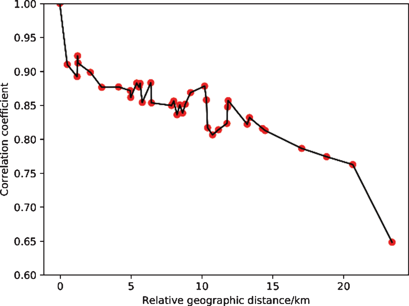
It can be seen from the figure that the correlation coefficient values are all above 0.6, so there is a strong positive correlation between the station to be predicted and other stations, and the overall performance shows that the longer the distance, the worse the correlation. Based on the researched correlation, this paper selects the appropriate correlation threshold through subsequent experiments and integrates the data of the stations to be predicted and the data of adjacent stations whose correlation coefficient is greater than the threshold for the input data of the prediction algorithm.
3Network model
3.1Time-series CNN
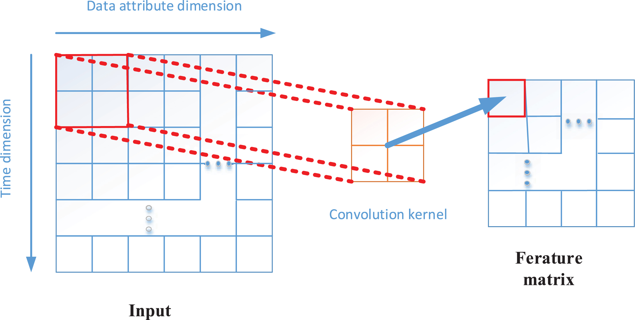
In recent years, Convolutional Neural Networks (CNN) have performed well in computer vision applications, especially for grid data such as images, which have demonstrated strong feature learning capabilities. Sparse weights, parameter sharing, and equivariant representation are the three major characteristics of CNN. These characteristics significantly reduce the complexity of the model and improve computational efficiency [28]. However, it is relatively rare to apply it to non-image time series data. It is often necessary to arrange and expand the time series data in a certain form on the plane, convert it into a similar grid structure, and then input it into the network. There are two ways to expand time series data. The first is to expand from left to right in chronological order. Zhang Guiyong (2016) used CNN to predict the stock index by processing the input time series data into the form of (k * t), Where t is the time step, k is the stock data, and k is 1 in the original text; another form of expansion is to expand from top to bottom in chronological order. Du Changshun et al. (2017) explored CNN in text sentiment analysis In the application, each word in a sentence is arranged from top to bottom, and the final format of the data is (k * t), where k is a word vector representing each word and t is a time step. In the application scenario of this article, the air quality data with k-dimensional attributes at t consecutive timesteps needs to be used as the input of the convolutional neural network. The expansion form is: from top to bottom according to time, and the attributes are expanded from left to right. Finally, a feature matrix containing spatial information is output through the convolution operation, as shown in Fig. 2. The specific convolution formula is as follows:
(3)
where v is the output feature matrix, n represents the number of input feature matrices, Xi is the input feature matrix, Wi represents the corresponding convolution kernel, dot represents the dot product operation of the two matrices, f is the activation function.
Fig. 2
Schematic diagram of time series convolution operation.
3.2Bidirectional LSTM
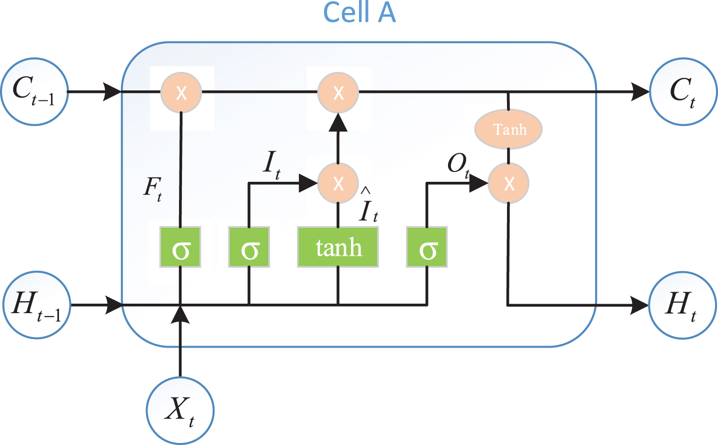
LSTM is a special type of recurrent neural network that can capture long-distance dependencies. It was proposed by Hochreiter and Schmidhuber in 1997 [29]. It aims to solve long-term dependency problems by means of short-term memory. Because LSTM can learn what information to remember and what to forget through the training process, it can even process very long sequence data without gradients disappearing. Now, LSTM is widely used to solve sequence data problems, such as speech recognition. The cells in LSTM have a complex cyclic structure, and information is added or deleted through the Gates structure, which selectively allows information to pass. Its structure is shown in Fig. 3. The LSTM cell has three gate structures for maintaining and updating the cell state, including the input gate, forget gate, and output gate. The input gate is designed to control the writing of input information to the memory, while the forget gate and output gate determine whether to save or release information from the memory at each decision point. The calculation formulas for each gate, storage cells, and hidden output layer height are as follows:
(4)
(5)
(6)
(7)
(8)
(9)
Fig. 3
LSTM cell A structure.
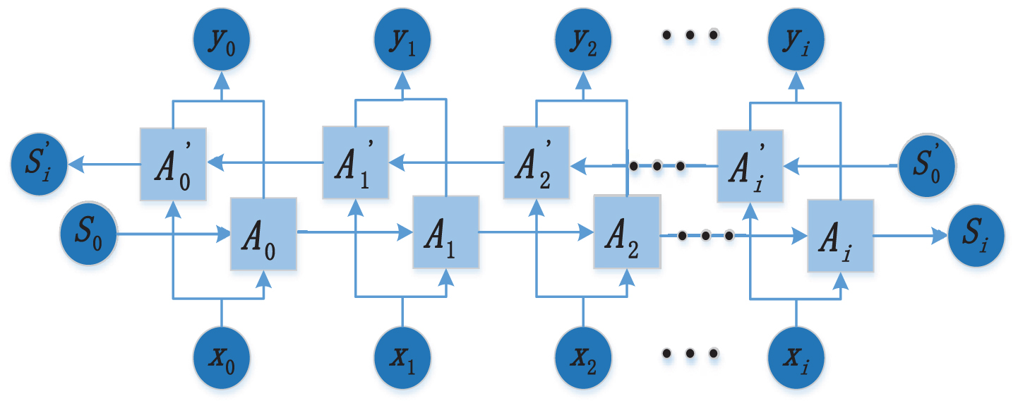
But there is still a problem with LSTM modeling: the information from back to front cannot be obtained. In some cases, the prediction may need to be determined jointly by the preceding inputs and the following inputs, which will be more accurate. Therefore, Schuster proposed the bidirectional LSTM (Bi-LSTM) model in 1997 to solve the problem that the unidirectional LSTM cannot handle the simultaneous capture of data information before and after [30]. The basic idea of the Bi-LSTM is to first calculate forward in each training sequence of the Forward layer, obtain and save the output of the forward hidden layer at each moment, and then calculate backward in the Backward layer along the time to obtain and save each moment. Finally, combine the output of the Forward layer and Backward layer at each moment as the final output. The overall structure is shown in Fig. 4, in which the hidden layer units Ai and
Fig. 4
Bidirectional LSTM structure diagram.
3.3A prediction model based on temporal and spatial features
The network structure of this article is shown in Fig. 5, which mainly includes three parts: the use of convolutional layers to extract spatial features between data; the extracted feature vector containing multiple time steps is input into the Bi-LSTM to extract temporal features; after the obtained feature vector passes through the fully connected layer, a prediction value is finally output.
Fig. 5
CNN+BiLSTM network structure diagram.
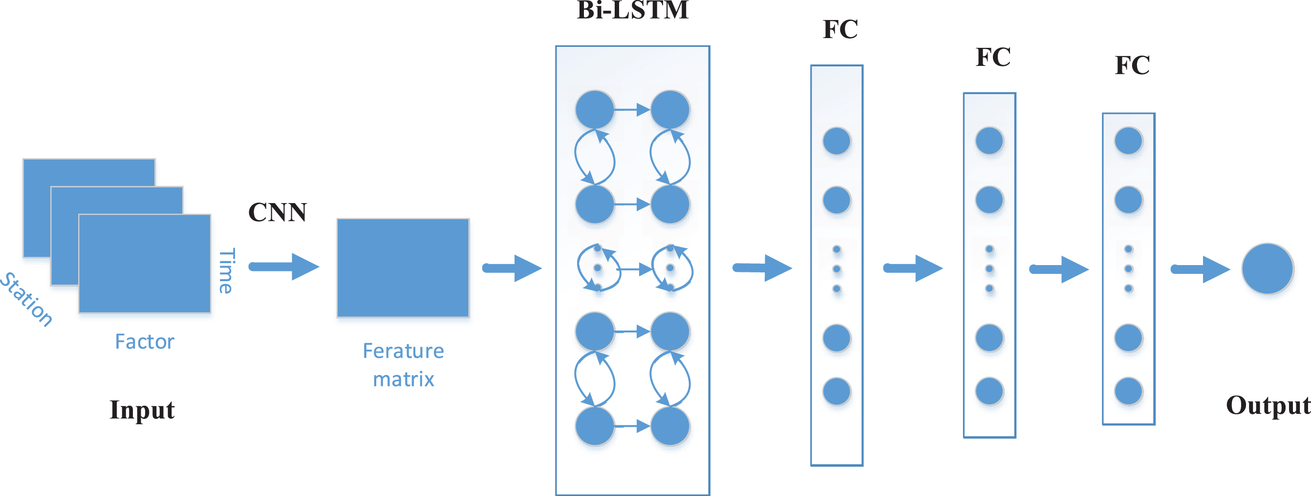
The single data input size in this paper is (t, k, n), that is, the input feature matrix has n channels, and the size of each channel is (t, k), where t is the time step, is the number of input factors, and n is the number of selected adjacent stations. First, a layer of 2D convolution layers with a convolution kernel size of (1, k) is used to extract the spatial features of the data, including the features between different stations data and the data between each attribute in the input Feature, the final calculation is a multi-channel feature matrix, each feature matrix size is (t, 1). Then, the obtained feature matrix is spliced according to the time dimension, and input a Bi-LSTM layer to extract the temporal features containing the data information before and after, the size is (t, 1), where l is the number of Bi-LSTM layer units. Finally, through the fully connected layer, the previously obtained feature vectors are integrated into the final predicted value of pm2.5, where multiple fully connected layers are used to improve the model’s nonlinear expression ability.
4Experiment and discussion
4.1Hyperparameter selection
In deep neural networks, choosing the right hyperparameters is a difficult but extremely important step, which directly affects the performance of neural network models. After comparing through a series of experiments: First, it is determined that the basic architecture of the network includes a convolutional layer, a bidirectional LSTM layer, and three fully connected layers. This network structure achieves the best training effect. Among them, the size of the convolution kernel in this article is set to (1, 7) to ensure that the convolution kernel slides along the time axis when the convolution operation is performed. According to previous studies, a small time step size cannot guarantee that the model has sufficient long-term memory input, while a larger time step size will increase irrelevant input and increase the amount of calculation. Therefore, this paper integrates the actual training effect and finally sets the time step size to 5. This paper uses adaptive moment estimation (Adam) as the optimizer to improve training speed. At the same time, relu is used as the activation function which avoids the problem of gradient disappearance and accelerates the network convergence process. The final selection of optimal model hyperparameters is shown in Table 1.
Table 1
Hyperparameter selection table
| Parameter | Description | Value |
| learning_rate | Learning rate of adam optimization algorithm | 0.001 |
| time_step | Time step of neural network input data | 5 |
| Epochs | The number of times to train the entire sample set | 200 |
| batch_size | The number of data used for each training | 80 |
| conv_filters | The number of convolution kernels in the convolution layer | 7 |
| kernel_size | The size of the convolution kernel | (1,7) |
| lstm_size | The number of Bi-LSTM layer units | 200 |
| dense1 | The number of nodes in the first layer of fully connected neural networks | 60 |
| dense2 | The number of nodes in the second layer of fully connected neural networks | 15 |
| dense3 | The number of nodes in the third layer of fully connected neural networks | 1 |
4.2Evaluation index of the model
After the structure of the model is determined, the training set is used to train the network until convergence. In order to evaluate the effectiveness of the model, three indicators are used in this paper, including mean absolute error (MAE), root mean square error (RMSE) and coefficient of determination (R2) [31].
1) MAE: Average absolute error is the average value of the absolute error between the true value of all single samples and the model prediction value, which can better reflect the true situation of the prediction error. The calculation formula is as follows:
(10)
2) RMSE: Root mean square error is the square root of the sum of the square of the difference between the true value of the sample and the predicted value of the model and the total number of samples N. It is very sensitive to extra large and small errors, and can well reflect the precision of the prediction error. The calculation formula is as follows:
(11)
3) R2: The coefficient of determination reflects the proportion of all the variation of the dependent variable that can be explained by the independent variable through the regression relationship. The closer the value of R2 is to 1, the better the independent variable can explain the dependent variable. The calculation formula is as follows:
(12)
In Eq. (10) to Eq. (12), N is the sample size, reali and predicti represent the real value and predicted value at time i, respectively;
4.3The influence of the selection of related stations on accuracy
In this experiment, for station A to be predicted, based on the correlation coefficient calculated between station A and other stations, the impact of setting different correlation coefficient thresholds on the model accuracy is analyzed and discussed. The experimental results are shown in Table 2.
Table 2
Comparison of model prediction effects under different correlation coefficient thresholds
| Thresholds | MAE | RMSE | R2 | Stations |
| 0.95 | 8.17 | 13.53 | 0.88 | 0 |
| 0.92 | 7.39 | 12.57 | 0.90 | 1 |
| 0.90 | 6.58 | 11.61 | 0.91 | 3 |
| 0.89 | 6.69 | 11.92 | 0.92 | 5 |
| 0.88 | 6.22 | 10.46 | 0.92 | 8 |
| 0.87 | 7.09 | 12.64 | 0.90 | 13 |
| 0.86 | 7.40 | 12.19 | 0.91 | 23 |
It can be seen from the table that when the similarity threshold is selected too high or too low, the final model effect will be worse, but the effect is better than when the similarity threshold is 0.95, that is, the model obtained when no adjacent site is used. So it can be concluded: Adding data from adjacent stations will increase the number of important features, which can improve the accuracy of the model during prediction. However, after adding too many sites, the data volume will become larger and larger, which will lead to irrelevant data and reduces the accuracy of the model. At the same time, when the set similarity threshold is 0.88, the obtained model has the best effect.
This paper studies the prediction model for a single station, so the final selection of a set of related station data with the best prediction effect is used to analyze and verify the prediction effect of our network model, that is, the similarity threshold is 0.88 and the number of adjacent stations is 8.
4.4Comparison and analysis of model prediction performance
In order to verify the prediction performance of this model, a support vector regression (SVR) model and seven deep learning models were used to analyzes the prediction effect, including the GRNN model, CNN model, Bi-LSTM model, LSTME model, STDNN model, CNNs-GRU model and the model in this article. Table 3 shows the MAE, RMSE and R2 of these models on the test set. We can see that compared with non-deep learning methods, the prediction errors of deep learning methods are significantly lower, mainly because pollutant data and weather data have strong nonlinearity, and non-deep learning methods are relatively weak in extracting nonlinear features. Secondly, compared with the GRNN, CNN, and Bi-LSTM networks that only consider the current station, the prediction effects of LSTME, CNNs-GRU, and our model that integrate data from neighboring stations have been significantly improved. Among them, the mae and rmse of our model is the smallest. The main reason is: compared with the LSTME model, we have merged the appropriate number of adjacent station data through correlation analysis, thereby reducing the impact of the data of weakly correlated stations; Compared with CNNs-GRU, we not only consider the spatial and temporal features of the adjacent station data, we also extract the local features that exist between the pollutant data and the weather auxiliary data through CNN. The R2 value of this model has reached 0.92, which also shows that the predicted value has a good explanation for the true value.
Table 3
Comparison of prediction effects of different models
| Model | MAE | RMSE | R2 |
| SVR | 24.05 | 29.91 | 0.73 |
| ARMA | 20.05 | 26.91 | 0.75 |
| GRNN | 16.79 | 21.95 | 0.81 |
| Bi-LSTM | 10.12 | 15.77 | 0.84 |
| CNN | 9.64 | 15.14 | 0.85 |
| LSTME | 8.20 | 13.24 | 0.88 |
| CNNs-GRU | 7.70 | 11.87 | 0.90 |
| Ours | 6.22 | 10.46 | 0.92 |
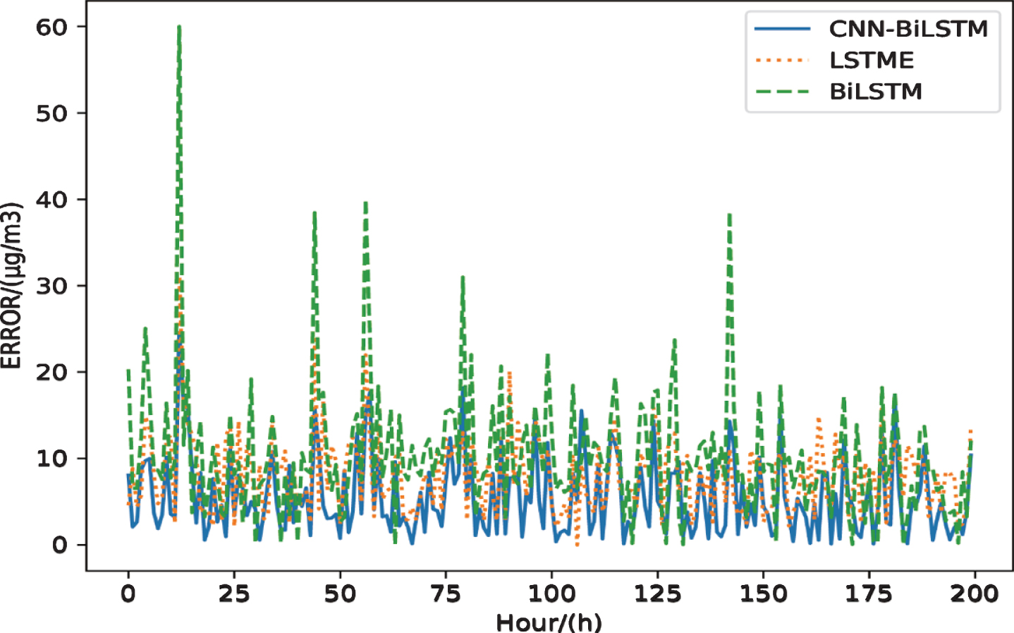
At the same time, to verify the effectiveness of the fusion of adjacent station data to improve the prediction accuracy, we draw the error graphs of the Bi-LSTM, LSTME, and our model, and intercept a certain period for observation, as shown in Fig. 6, where the ordinate error is the absolute value of the difference between the predicted value and the true value. It can be seen that the overall error of our model is smaller than that of the other two models; at the same time, at some sudden changes in the error value, the magnitude of the error mutation of our model is also small, mainly because the convolutional network is used in this paper to learn the local characteristics of the multi-station data. When the current station data is abnormal, the impact can be well reduced. Secondly, the overall error of our model fluctuates significantly less than the other two models. Therefore, the model in this paper has good predictive performance, and at the same time has a small response to outliers, and has good predictive robustness.
Fig. 6
Comparison error graph of the model in this paper, Bi-LSTM model and LSTME model.
In this paper, we have considered multiple influencing factors data, including season, temperature, humidity, pressure at the detection station, wind speed and direction, etc. To verify the impact of these data on the prediction accuracy, the data set was reorganized, and the model in this paper was used to train the data set containing influencing factors and not containing influencing factors. The results are shown in Table 4. It can be seen that after using the data of influencing factors, the prediction effect has been significantly improved.
Table 4
Comparison of the impact of influencing factor data on prediction performance
| Influencing factor data | MAE | RMSE | R2 |
| Not added | 11.49 | 15.26 | 0.85 |
| Added | 6.22 | 10.46 | 0.92 |
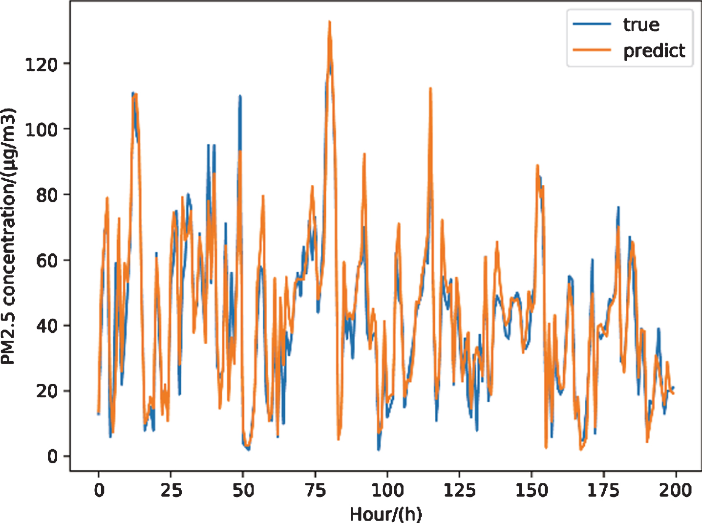
The final prediction effect of our hybrid model on the test set of this paper is shown in Fig. 7. In the figure, the abscissa is time in hours, the ordinate is PM2.5 concentration, the blue broken line is the actual value of the concentration measured by the device, and the orange broken line is the predicted value of the algorithm in this paper. It can be seen that the model has a strong tracking performance for the changing trend of pm2.5.
Fig. 7
The prediction effect of our hybrid model.
4.5Analysis of long-term prediction performance
In the actual application of PM2.5 prediction, it is of little significance to the regional warning that only predicting the concentration value in the next hour. Therefore, it is necessary to continuously forecast the data for some time in the future. To further test the prediction performance of the method proposed in this paper on a long-term scale, we have compared and analyzed the MAE values of the results of multiple models in continuous forecasting of the next 5 hours of data. The results are shown in Table 5. It can be seen from the results that although the error of all methods increases with the increase of the prediction time, the prediction error of the deep learning method is still significantly smaller than that of the non-deep learning method. At the same time, compared with Bi-LSTM and CNN, the error increase of the model using adjacent station data is smaller, indicating that adding adjacent station data can effectively improve the long-term prediction performance of the model. When predicting multi-hour data, our model maintains the minimum MAE value, which indicates that the model in this paper has high accuracy and stability in long-term prediction performance.
Table 5
Comparison of long-term prediction performance
| MAE | 1 | 2 | 3 | 4 | 5 |
| SVR | 24.05 | 28.36 | 33.38 | 35.06 | 41.91 |
| ARMA | 20.05 | 24.61 | 27.78 | 32.49 | 35.25 |
| GRNN | 16.19 | 19.41 | 21.62 | 24.74 | 26.41 |
| Bi-LSTM | 10.12 | 13.62 | 15.17 | 18.28 | 21.39 |
| CNN | 9.64 | 12.17 | 15.24 | 19.30 | 22.43 |
| LSTME | 8.20 | 10.84 | 12.61 | 14.95 | 17.43 |
| CNNs-GRU | 7.70 | 9.15 | 10.44 | 12.65 | 15.37 |
| Ours | 6.22 | 7.36 | 9.28 | 12.45 | 14.80 |
5Conclusion
In this paper, we propose a hybrid model based on CNN and Bi-LSTM, which is used to predict the PM2.5 of air pollutants in the urban area of Fushun. First of all, the historical data of all the stations in Fushun city are analyzed for correlation. After experimental comparison, a group of adjacent stations with a higher correlation coefficient with the station to be predicted are selected, and the PM2.5 data, weather data, and month data of these stations are integrated as input to the network. Secondly, based on the proposed hybrid model, we used CNN to effectively extract the spatial characteristics of data between different stations and the internal characteristics between different attributes; at the same time, we used Bi-LSTM to obtain the bidirectional time features before and after, and finally obtained a more accurate and stable prediction effect. Through performance evaluation and comparison of results, the main findings of this paper are as follows: The addition of neighboring station data for prediction improves the accuracy of the model while also minimizing the impact of outliers; multiple influencing factors are added to improve the prediction accuracy of the model; this model can effectively extract the temporal and spatial features of the data through CNN and Bi-LSTM, and it also has high accuracy and stability in long-term prediction performance.
We only considered the performance of the prediction model and ignored the impact of increased calculation and time consumption brought by the addition of adjacent station data. Next, we will conduct in-depth research on improving the time performance of the model. For example, when selecting a correlation coefficient thresholds, considering prediction performance and time consumption to reduce the amount of data input, and considering using 3D-CNN to replace the convolutional layer in the current structure to reduce the amount of calculation, these ideas have a certain value and can be further verified.
References
[1] | Kampa M. and Castanas E. , Human health effects of air pollution, Environ Pollut 151: (2) ((2008) ), 362–367. |
[2] | Zheng Y. , Yi X. , Li M. , et al., Forecasting fine-grained air quality based on big data. Proceedings of the 21th ACM SIGKDD International Conference on Knowledge Dis-covery and Data Mining. ACM, 2015, pp. 2267–2276. |
[3] | Chen J. , Lu J. , Avise J.C. , et al., Seasonal modeling of PM 2.5 in California’s SanJoaquin Valley, Environ 92: ((2014) ), 182–190. |
[4] | Forecasting urban PM10 and PM2.5 pollution episodes in very stable nocturnal conditions and complex terrain using WRF–Chem CO tracer model, Atmos Environ. |
[5] | A nested air quality prediction modeling sys-tem for urban and regional scales: application for high-ozone episode in Taiwan, Water Air Soil Pollut. |
[6] | Khemet B. and Richman R. , A univariate and multiple linear regression analysis on a national fan (de) Pressurization testing database to predict airtightness in houses[J], Building and Environment, 2018, 146. |
[7] | Mauricio J.A. , Algorithm AS 311: The Exact Likelihood Function of a Vector Autoregressive Moving Average Model[J], Journal of the Royal Statistical Society, Series C (Applied Statistics) 46: (1) ((1997) ). |
[8] | Zhi-Guo L. and Tao W. , Air Traffic Flow Prediction Based on Least Squares Support Vector Regression[J], Energy Procedia, 2011, 11. |
[9] | Paschalidou A.K. , Karakitsios S. , Kleanthous S. , et al., Forecasting hourly PM10 concentration in Cyprus through artificial neural networks and multiple regression models: Implications to local environmental management[J], Environmental Science & Pollution Research 18: (2) ((2011) ), 316–327. |
[10] | Zhou Y. and Qiu G. , Random forest for label ranking[J], Expert Systems With Applications 2018, 112. |
[11] | Natarajan U. , Saravanan R. and Periasamy V.M. , Erratum to: Application of particle swarm optimisation in artificial neural network for the prediction of tool life[J], The International Journal of Advanced Manufacturing Technology 90: (5-8) ((2017) ). |
[12] | Tkachenko R. , Izonin I. , Kryvinska N. , Dronyuk I. and Zub K. , An Approach towards Increasing Prediction Accuracy for the Recovery of Missing IoT Data based on the GRNN-SGTM Ensemble, Sensors 20: ((2020) ), 2625. |
[13] | Abdul-Wahab S.A. and Al-Alawi S.M. , Assessment and prediction of tropospheric ozone concentration levels using artificial neural networks[J],&219– 228, Software 17: (3) ((2002) ). |
[14] | Beckerman B.S. , Jerrett M. , Serre M. , Marting R.V. , Lee S.J. , Van D. , Ross Z. , Su J. and Burnett R.T. , Environment, Science & Technology 47: ((2013) ), 7233–7241. |
[15] | Feng Y. , Zhang W. , Sun D. , et al., Ozone concentration forecast method based on genetic algorithm optimized back propagation neural networks and support vector machine data classification, Environ 45: (11) ((2011) ), 1979–1985. |
[16] | Xayasouk T. , Lee H.M. and Lee G. , Air Pollution Prediction Using Long Short-Term Memory (LSTM) and Deep Autoencoder (DAE) Models, 12: (6) ((2020) ). |
[17] | Hochreiter S. , The Vanishing Gradient Problem During Learning Recurrent Neural Nets and Problem Solutions[J], International Journal of Uncertainty, Fuzziness and Knowledge-Based, Systems 6: (2) ((1998) ), 107–116116. |
[18] | Lei F. , Gu D. and Wang X. , Prediction model of air pollutant concentration based on deep neural network: A case study of Fushun, Liaoning Province[J], IOP Conference Series Earth and Environmental Science 467: ((2020) ), 012151. |
[19] | Li X, Peng L, Yao X, et al., Long short-term memory neural network for air pollutant concentration predictions: Method development and evaluation[J], Environmental Pollution 231: (pt.1) ((2017) ), 997–1004. |
[20] | Soh P.-W. , Chang J.-W. and Huang J.-W. , Adaptive deep learning-based air quality pre-diction model using the most relevant spatial-temporal relations, IEEE Access 6: ((2018) ), 38186–38199. |
[21] | Xie H. , Ji L. , Wang Q. and Jia Z. , Research of PM2.5 Prediction System Based on CNNs-GRU in Wuxi Urban Area, IOP Conference Series: Earth and Environmental Science 300: ((2019) ), 032073. 10.1088/1755-1315/300/3/032073. |
[22] | Ao D. , Cui Z. and Gu D. , Hybrid model of Air Quality Prediction Using K-Means Clustering and Deep Neural Network, (2019), 8416–8421. 10.23919/ChiCC.2019.8865861. |
[23] | Tkachenko R. , Izonin I. , Kryvinska N. , Dronyuk I. and Zub K. , An approach towards increasing prediction accuracy for the recovery of missing iot data based on the grnn-sgtm ensemble. Sensors (Switzerland), Volume, 20: , (2020) . |
[24] | Izonin I. , Gregušml M. , Tkachenko R. , et al., SGD-Based Wiener Polynomial Approximation for Missing Data Recovery in Air Pollution Monitoring Dataset[M], Advances in Computational Intelligence, 2019. |
[25] | Izonin I. , Tkachenko R. , Kryvinska N. , Zub K. , Mishchuk O. and Lisovych T. , Recovery of Incomplete IoT Sensed Data using High-Performance Extended-Input Neural-Like Structure, Comput Sci 160: ((2019) ), 521–526. doi: 10.1016/j.procs.2019.11.054. |
[26] | Pak U. , Ma J. , Ryu U. , Ryom K. , Juhyok U. , Pak K. and Pak C. , Deep learning-based PM2.5 prediction considering the spatiotemporal correlations: A case study of Beijing, China, Science of The Total Environment 699: ((2019) ). 10.1016/j.scitotenv.2019.07.367. |
[27] | Zhou H. , Deng Z. , Xia Y and Fu M. , A new sampling method in particle filter based on Pearson correlation coefficient[J], Neurocomputing, 2016, 216. |
[28] | Bengio Y.I. , Goodfellow J. and Courville A. , Deep Learning. MIT Press, Cambridge, MA, 2017(1) ((2016) ), 173–179. |
[29] | Hochreiter S. and Schmidhuber J. , Long short-term memory[J], Neural Computation 9: (8) ((1997) ), 1735–1780. |
[30] | Schuster M. and Paliwal K.K. , Bidirectional recurrent neural Networks[J], IEEE Transactions on Signal Processing 45: (11) ((1997) ), 2673–2681. |
[31] | Bobyr M.V. and Emelyanov S.G. , A nonlinear method of learning neuro-fuzzy models for dynamic control systems[J], Applied Soft Computing Journal 2020, 88. |


