
Fuzzy mixed graphs and its application to identification of COVID19 affected central regions in India
Abstract
In the recent phenomenon of social networks, both online and offline, two nodes may be connected, but they may not follow each other. Thus there are two separate links to be given to capture the notion. Directed links are given if the nodes follow each other, and undirected links represent the regular connections (without following). Thus, this network may have both types of relationships/ links simultaneously. This type of network can be represented by mixed graphs. But, uncertainties in following and connectedness exist in complex systems. To capture the uncertainties, fuzzy mixed graphs are introduced in this article. Some operations, completeness, and regularity and few other properties of fuzzy mixed graphs are explained. Representation of fuzzy mixed graphs as matrix and isomorphism theorems on fuzzy mixed graphs are developed. A network of COVID19 affected areas in India are assumed, and central regions are identified as per the proposed theory.
1Introduction
Graph theory is the study of interactions among nodes (or vertices). The idea of graphs was initiated by Euler in 1973 to solve the Konigsberg bridge problem. After that, many branches have been developed. One of the essential branches is to study the mixed graphs where the graphs consider directed and undirected edges both. Let us consider V (non-empty) be a set of elements, called vertices. Also let, E = E1 ∪ E2 where E1 ⊂ V × V is a set of unordered pairs of vertices, i.e., E1 = {(u, v) |u, v ∈ V}, called a set of undirected edges and
The study of mixed graphs [1] was started in 1970. Sotskov and Tanaev (1976) discussed the colouring of mixed graphs [2]. Liu and Li (2015) introduced Hermitian-adjacency matrices of mixed graphs [3]. Adiga et al. (2016) studied on adjacency matrix [4] of mixed graphs. Mohammed (2017) studied on mixed graph representation and isomorphism [5]. There are many applications of mixed graphs on social networks. For example, Facebook network [6] allow mixed direction, since if one friend follows other, then there will be directed edges in a mentioned direction and there will be an undirected edge if they are friends to each other. Samanta et al. [7] introduced another type of mixed graph, called a semi-directed graph and studied competitions on these graphs.
Sometimes vertices (persons) and the relationship between them may not precisely define. So there may be fuzziness [8, 9] in the graph. The idea of fuzziness to graph theory [10] first introduced by Kauffmann (1973) and after that modification of fuzzy graphs [11] developed by Rosenfeld (1975). The homomorphism, isomorphism, automorphism [12] on fuzzy graphs were developed by Bhutani (1989). The operations [13] like the cartesian product, union, join etc. on fuzzy graphs were studied by Mordeson and Peng (1994). There were various related studies on fuzzy digraphs [14]. Akram and Dubek (2011) introduced interval-valued fuzzy graphs [15] where membership values of vertex and edges are interval. In [16], Akram proposed bipolar fuzzy graphs. There are various studies on bipolar fuzzy graphs [17–19]. The concepts of planer graph [20] under fuzzy environment was introduced by Samanta and Pal (2015). The concepts of the fuzzy environment in food web studied by Samanta and Pal (2013) and represented fuzzy competition graph [21] more realistically. After that, as a generalization of the fuzzy graph, Samanta and Sarkar (2016, 2018) proposed the generalized fuzzy graph [22] and generalized fuzzy competition graph [23]. Akram and Sarwar [24] studied on fuzzy graph structures [25, 26] and applications. More relevant studies on fuzzy graphs can be found in [27–32, 33–40]. The chronological contributions of authors towards fuzzy mixed graphs are presented (Table 1).
Table 1
Contributions of authors
| Year | Authors name | Contribution |
| 1970 | N. V. Lambin and V. S Tanaev | Introduction of mixed graph. |
| 1973 | Kaufmann | Fuzziness to graph theory. |
| 1975 | Rosenfeld | Modification to fuzzy graph definition. |
| 1994 | J.N. Mordeson and C.S Peng | Operations on fuzzy graphs. |
| 1996 | J. N. Mordeson and P. S. Nair | Fuzzy digraphs and finite state machines. |
| 2016 | S. Samanta and B. Sarkar | Introduced generalized fuzzy graph. |
| 2016 | C. Adiga et al. | Studied on adjacency matrix of mixed graphs. |
| 2020 | C. Yang and Y. Lee | Mixed graphs and Facebook network. |
| 2020 | S. Samanta et al. | Introduced a special type of mixed graph, called a semi-directed graph. |
| This paper | K. Das et al. | Introduction of fuzzy mixed graph and properties. |
Thus there are huge developments on fuzzy graphs which are undirected or directed, but both types of edges not considered in a single graph. The mixed graphs are better to represent some special types of networks where both types of edges occur simultaneously like brain network, research networks, etc. But these networks contain lots of ambiguity. The ambiguity occurs in not only to the connectedness but also to the directedness. One node may strongly dominate to other connected nodes. Thus our main aim is to develop the mixed graph in fuzzy environments where the membership values of vertices, membership values of undirected edges, membership values of directed edges with the value of directedness have been considered. In this study, some operations, completeness, matrices presentation, and isomorphism, competitions on fuzzy mixed graphs are developed. An application of fuzzy mixed graph in a network of COVID19 affected regions in India has been shown.
Therefore the major contributions of this study are pointed out below:
• The fuzzy mixed graphs are introduced as a generalization of mixed graphs.
• Operations on fuzzy mixed graphs are studied.
• Adjacency matrices, incidence matrices of fuzzy mixed graphs are presented.
• Isomorphism with properties of fuzzy mixed graphs is improved.
• A numerical example of a fuzzy mixed graph in a network of COVID19 affected regions in India has been shown.
2Fuzzy mixed graph (FMG)
To discuss fuzzy mixed graphs, the definition of fuzzy graphs is given first. Let V be a non-empty set. Then G = (V, σ, μ) is said to be a fuzzy graph if there exists a function μ : V → [0, 1], such that
(1)
Definition 2.1. Let V be a non-empty set. Then G = (V, E1, E2, μ1, μ2, σ, δ) is said to be fuzzy mixed graph if there exist functions σ : V → [0, 1], μ1 : E1 → [0, 1] μ2 : E2 → [0, 1] , δ : E2 → [0, 1] such that
• Note that the measure of directedness is one kind of measure of domination/direction. If two equal powerful nodes are connected, then they may not influence/direct each other. If a low powerful node is connected to a highly powerful node, then the later node can dominate the first one by their power difference. This motivates us to define the measure of directedness as
• Note that every undirected edge is represented by the value μ1 ∈ [0, 1] only and every directed edge is represented by the value (μ2, δ).
• The comparison of existing fuzzy graphs and fuzzy mixed graphs is described as follows.
In fuzzy graphs, edges are undirected and in fuzzy di-graphs edges are directed with the following property that edge membership values are less than or equal to the minimum of end vertex membership values.
In fuzzy mixed graphs, edges may be both directed and /or undirected with the property that edge membership values are less than or equal to the minimum of end vertex membership values. Additionally, in fuzzy mixed graphs, the measure of directedness is added to directed edges with the property that measure of directedness iless than or equal to the absolute difference of end vertex membership values.
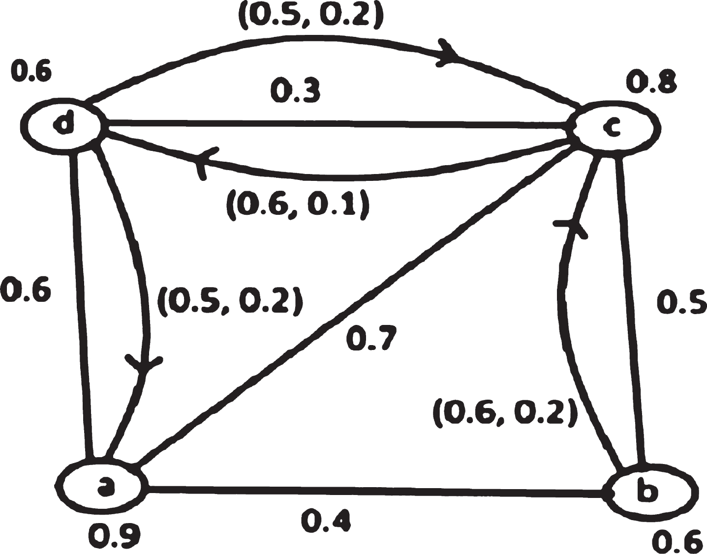
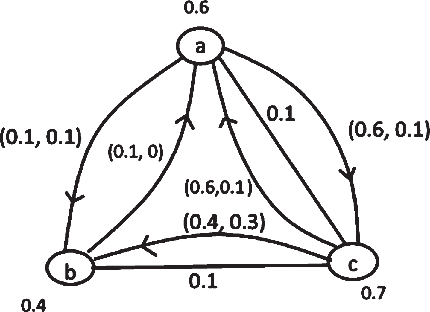
Example 2.2. We consider a graph with four vertices a, b, c, d and nine edges (Fig. 1). All vertices and edges satisfy all the restrictions defined in Definition. 2.1.; hence it is a fuzzy mixed graph.
Fig. 1
Example of a fuzzy mixed graph.
Definition 2.3. A fuzzy mixed walk in a FMG
Example 2.4. Consider a fuzzy mixed graph (Fig. 1). Here a - b → c ← d is a fuzzy mixed walk and hence a fuzzy mixed path. Also, a - b → c - d → a is a fuzzy mixed cycle.
Definition 2.5. The fuzzy mixed degree FMD (v). of a vertex v in the fuzzy mixed graph G = (V, E1, E2, μ1, μ2, σ, δ) is defined by
Example 2.6. We consider a fuzzy mixed graph (Fig. 1). The fuzzy mixed degree of a vertex c. is I (c) = (0.3 + 0.5) + (0.6 + 0.6 × 0.2 + 0.5 + 0.5 × 0.2) - (0.6 + 0.6 × 0.1) = 1.46.
Definition 2.7. Let G = (V, E1, E2, μ1, μ2, σ, δ) be a fuzzy mixed graph. Then a fuzzy graph
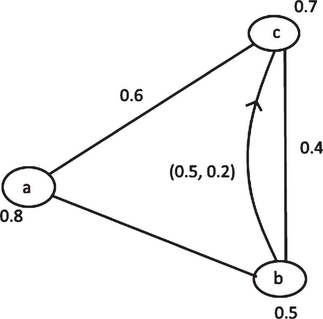
Example 2.8. Consider a fuzzy mixed graph H (Fig. 2). Hence it is a fuzzy mixed subgraph of a fuzzy mixed graph G (Fig. 1) as it satisfies all the conditions.
Fig. 2
A z mixed subgraph.
Definition 2.9. Let G = (V, E1, E2, μ1, μ2, σ, δ) be a fuzzy mixed graph. Then the order of Gis∑v∈Vσ (v) and size of G is
Example 2.10. We consider a fuzzy mixed graph in Fig. 1. Then its order is 2.9, and the size is (2.5, 2.2, 0.7).
3Operations on FMG
Definition 3.1. Let G = (V, E1, E2, μ1, μ2, σ, δ) and
where X = V× V′ = { (v, v′) : v ∈ V, v′ ∈ V′ }
Theorem 3.2. Let G = (V, E1, E2, μ1, μ2, σ, δ) and
Proof. Since
Similarly,
Aain,
Similarly
This completes the proof.
Definition 3.3. Let G = (V, E1, E2, μ1, μ2, σ, δ) and
Theorem 3.4. Let G = (V, E1, E2, μ1, μ2, σ, δ) and
Proof. Case-I: Let
Then
= min{ (σ ∪ σ′) (x) , (σ ∪ σ′) (y) } if x, y ∈ V - V′.
Again
= min{ (σ ∪ σ′) (x) , (σ ∪ σ′) (y) } if x ∈ V - V′, y ∈ V ∩ V′
Case-II: Let
Case-III: Let
Then
Case-IV: Let
Now,
Case-V: Let
Now
Case-VI: Let
Now
This completes the proof.
Definition 3.5. Let G = (V, E1, E2, μ1, μ2, σ, δ) and
(σ + σ′) (x) = (σ ∪ σ′) (x) for all x ∈ V ∪ V′
Theorem 3.6. Let G = (V, E1, E2, μ1, μ2, σ, δ) and
Proof. Case-I: Let
Now, if
Case-II: Let
Now, if
Case-III: Let
Now, if
This completes the proof.
4Complete FMG
Definition 4.1. If there exist all three types of connections, i.e. out-directed edges, in-directed edges and undirected edges between every pair of vertices in the fuzzy mixed graph G = (V, E1, E2, μ1, μ2, σ, δ) and
Then the graph is called a complete fuzzy mixed graph.
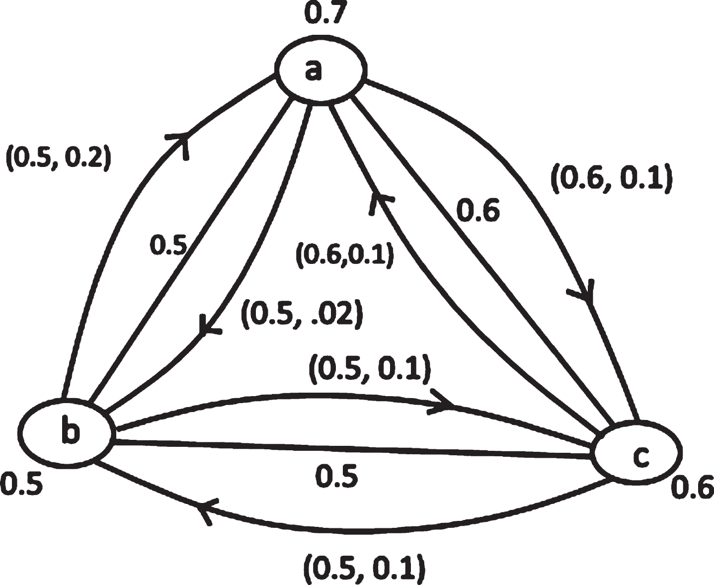
Example 4.2. A complete FMG is assumed in Fig. 3. Between every pair of vertices, there exist all three types of edges with specified membership values.
Fig. 3
A complete fuzzy mixed graph.
Definition 4.3. A fuzzy mixed graph is called regular if the fuzzy mixed degrees of all vertices are equal. That is FMD (k) = constant, for all k ∈ V.
Note 4.4 Every complete fuzzy mixed graph may not be regular. A fuzzy mixed graph given in Example 4.2 is complete, but it is not regular.
Definition 4.5. Let G = (V, E1, E2, μ1, μ2, σ, δ) be a FMG and
Example 4.6. We consider a fuzzy mixed graph G consisting of three vertices {a, b, c}. The membership values of vertices and edges are shown below in Fig. 4. The corresponding complement Gc of G is shown below in Fig. 5.
Fig. 4
A fuzzy mixed graph G
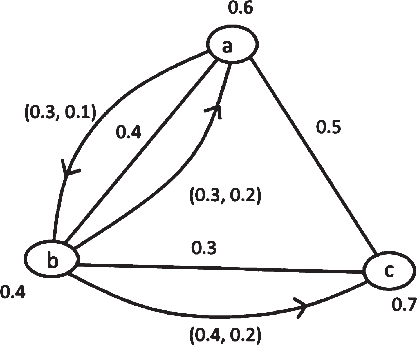
Fig. 5
Complement Gcof G.
Remark 4.7. The complement of a complete fuzzy mixed graph may not always be a null graph.
Theorem 4.8. The complement of the complement of a fuzzy mixed graph is again the same graph. If Gbeafuzzymixedgraphthen (Gc) c = G.
Proof. since
5Matrix representation of FMG
Two types of matrix representations of a fuzzy mixed graph are described below. One is the adjacency matrix, and another is the incidence matrix.
5.1Adjacency matrix
To find adjacency matrix of FMG, we define adjacency value ad (vi, vj) of vertex vi with vertex vj where
The adjacency matrix is n × n square matrix whose elements are
Now the adjacency matrix of a fuzzy mixed graph (Fig. 1) is given below.
| a | b | c | d | |
| a | (0,0,0) | (0.4,0,0) | (0.7,0,0) | (0.6,0.6,0) |
| b | (0.4,0,0) | (0,0,0) | (0.5,0,0.72) | (0,0,0) |
| c | (0.7,0,0) | (0.5,0.72,0) | (0,0,0) | (0.3,0.6,0.66) |
| d | (0.6,0,0.6) | (0,0,0) | (0.3,0.66,0.6) | (0,0,0) |
Observations:
i. Non-zero entries of the matrix (at least one component of the entry is non zero) indicate, there are some connections between the corresponding vertices. The connections may be undirected or directed.
ii. Zero entries (all components are zero) indicate that there does not exist any edge between the corresponding vertices.
An associated term adjacency number adn (vi, vj) is defined as follows.
5.2Incidence matrix
We define incidence value In (u, v) of the edge (
Then the incidence matrix of a fuzzy mixed graph (Fig. 1) is shown below.
| (a,b) | (b,c) | (a,c) | (c,d) | (a,d) | |
| a | (0.4,0,0) | (0,0,0) | (0.7,0,0) | (0,0,0) | (0.6,0,0.6) |
| b | (0.4,0,0) | (0.5,0.72,0) | (0,0,0) | (0,0,0) | (0,0,0) |
| c | (0,0,0) | (0.5,0,0.72) | (0.7,0,0) | (0.3,0.66,0.6) | (0,0,0) |
| d | (0,0,0) | (0,0,0) | (0,0,0) | (0.3,0.6,0.66) | (0.6,0.6,0) |
Observations:
i Non-zero entries of the matrix (at least one component of the entry is non zero) indicate, there are some connections between the corresponding vertex and edge.
ii Zero entries (all components are zero) indicate that there does not exist any connection between the corresponding vertex and edge.
6Isomorphism on FMG
Definition 6.1. Let G = (V, E1, E2, μ1, μ2, σ, δ) and
Definition 6.2 Let G = (V, E1, E2, μ1, μ2, σ, δ) and
If G and G′ are isomorphic, then we write G ≅ G′.
Remark 6.3. An isomorphism on fuzzy mixed graphs preserves both the weights of vertices and edges.
Definition 6.4 Let G = (V, E1, E2, μ1, μ2, σ, δ) and
Remark 6.5 A weak isomorphism on fuzzy mixed graphs preserves only the weights of vertices.
Definition 6.6 Let G = (V, E1, E2, μ1, μ2, σ, δ) and
Remark 6.7. A co-weak isomorphism on fuzzy mixed graph preserves only the weights of edges.
Theorem 6.8. If any two fuzzy mixed graphs are isomorphic, then their order and size are the same.
Proof. Let f be an isomorphism from G = (V, E1, E2, μ1, μ2, σ, δ) to
Again, since
Therefore the size of G is equal to the size of G′.
Theorem 6.9 If any two fuzzy mixed graphs are isomorphic, then fuzzy mixed degrees of their vertices are the same.
Proof. Let f be an isomorphism from G = (V, E1, E2, μ1, μ2, σ, δ) to
= FMD′ (f (vk)) which is the fuzzy mixed degree f (vk) ∈ V′.
This completes the proof.
Theorem 6.10 Two fuzzy mixed graphs are isomorphic if and only if their complements are isomorphic.
Proof. Let G = (V, E1, E2, μ1, μ2, σ, δ) and
Assume G ≅ G′. Then there exists a bijective mapping f : V → V′ such that
Now,
Similarly,
for all a, b ∈ V
Now,
Therefore, μ1 (a, b) = μ1′ (h (a) , h (b)) for all a, b ∈ V, since σ (a) = σ′ (h (a)) .
Similarly,
7Application to the identification of COVID19 affected central regions in India
To identify the central regions through the fuzzy mixed graph, a network of COVID19 affected regions in India are assumed. The data has been shown in Table 2. The node membership values are assumed proportional to the number of affected people in the region. For this case, the membership values are the normalized value of the number of affected people.
Table 2
Collected data of COVID19 in India from official website website https://www.mohfw.gov.in/ dated 12.06.2020
| Sr. No | States (INDIA) | Number of COVID19 affected People | Node membership values values |
| 1 | Maharashtra | 94041 | 1 |
| 2 | Tamil Nadu | 36841 | 0.39 |
| 3 | Delhi | 32810 | 0.35 |
| 4 | Telangana | 4111 | 0.04 |
| 5 | Kerala | 2161 | 0.02 |
| 6 | Rajasthan | 11600 | 0.12 |
| 7 | Uttar Pradesh | 11610 | 0.12 |
| 8 | Andhra Pradesh | 5269 | 0.06 |
| 9 | Madhya Pradesh | 10049 | 0.11 |
| 10 | Karnataka | 6041 | 0.06 |
| 11 | Gujarat | 21521 | 0.23 |
| 12 | Haryana | 5579 | 0.06 |
| 13 | Jammu and Kashmir | 4507 | 0.05 |
| 14 | West Bengal | 9328 | 0.1 |
| 15 | Punjab | 2805 | 0.03 |
| 16 | Odisha | 3250 | 0.03 |
| 17 | Bihar | 5710 | 0.06 |
| 18 | Uttarakhand | 1562 | 0.02 |
| 19 | Assam | 3092 | 0.03 |
The links between any two regions are based on the data collected from www.covid19india.org dated 12th June 2020. The membership values for the links are assumed as per the availability of data of mutual relation between the countries. The default case of the link membership values is the minimum of end vertex membership values. The edge membership values of directed edges are shown as the adjacency matrix in Table 3. Along with this, the measure of directedness has been shown in the same table. Also, the corresponding adjacency number is calculated. The membership values of undirected edges are shown in Table 4.
Table 3
Directed edge membership values of the network in Fig. 6
| Directed Edges | Membership values | Measure of directedness | Adjacency number |
| (3,2) | 0.35 | 0.04 | 0.36 |
| (3,7) | 0.12 | 0.23 | 0.15 |
| (3,9) | 0.11 | 0.24 | 0.14 |
| (3,13) | 0.05 | 0.3 | 0.07 |
| (3,14) | 0.1 | 0.25 | 0.13 |
| (3,15) | 0.03 | 0.32 | 0.04 |
| (3,17) | 0.06 | 0.29 | 0.08 |
| (3,18) | 0.02 | 0.33 | 0.03 |
| (3,19) | 0.03 | 0.32 | 0.04 |
| (5,2) | 0.02 | 0.37 | 0.03 |
| (5,8) | 0.2 | 0.04 | 0.21 |
| (5,10) | 0.02 | 0.04 | 0.02 |
| (6,1) | 0.12 | 0.88 | 0.23 |
| (6,11) | 0.12 | 0.11 | 0.13 |
| (10,1) | 0.06 | 0.84 | 0.11 |
| (1,7) | 0.12 | 0.88 | 0.23 |
| (1,17) | 0.06 | 0.94 | 0.12 |
| (1,16) | 0.03 | 0.97 | 0.06 |
| (1,14) | 0.1 | 0.9 | 0.19 |
| (2,7) | 0.12 | 0.27 | 0.15 |
| (2,17) | 0.06 | 0.33 | 0.08 |
| (2,16) | 0.03 | 0.36 | 0.04 |
| (2,14) | 0.1 | 0.29 | 0.13 |
| (11,7) | 0.12 | 0.11 | 0.13 |
| (11,17) | 0.06 | 0.17 | 0.07 |
| (11,16) | 0.03 | 0.2 | 0.0s4 |
| (11,14) | 0.1 | 0.13 | 0.11 |
| (1,3) | 0.35 | 0.65 | 0.58 |
| (1,6) | 0.12 | 0.88 | 0.23 |
| (1,15) | 0.03 | 0.97 | 0.06 |
| (1,11) | 0.23 | 0.77 | 0.41 |
| (1,5) | 0.02 | 0.98 | 0.04 |
| (1,9) | 0.11 | 0.89 | 0.21 |
Table 4
Undirected edge membership values of Fig. 6
| Undirected edges | Membership values | Adjacency number |
| (u, v) | μ1 (u, v) | |
| (3,6) | 0.32 | 0.32 |
| (4,9) | 0.22 | 0.22 |
| (4,16) | 0.04 | 0.04 |
| (7,9) | 0.22 | 0.22 |
| (9,14) | 0.1 | 0.1 |
To measure central regions of COVID19 affected states, a fuzzy mixed graph is considered with the above-mentioned data. The corresponding fuzzy mixed graphs have been shown in Fig. 6. Centrality measurement is essential in networks. There are lots of centrality measure [41] available in networks, including degree centrality. But degree centrality does not capture the notion of uncertainty and measure of directedness. Degree centrality only counts the direct effects of a directed link. For mixed graphs, degree centrality counts the out-directed links and the undirected links. This study introduces another measure of centrality, namely Fuzzy mixed degree centrality. Fuzzy mixed degree centrality is sum of the adjacency numbers of its adjacent edges. Based on this study, fuzzy mixed degree centrality is equivalent to degree centrality and captures uncertainty perfectly. The Fuzzy mixed degree centralities of all nodes have been shown in Table 5.
Fig. 6
COVID19 affected network in India.
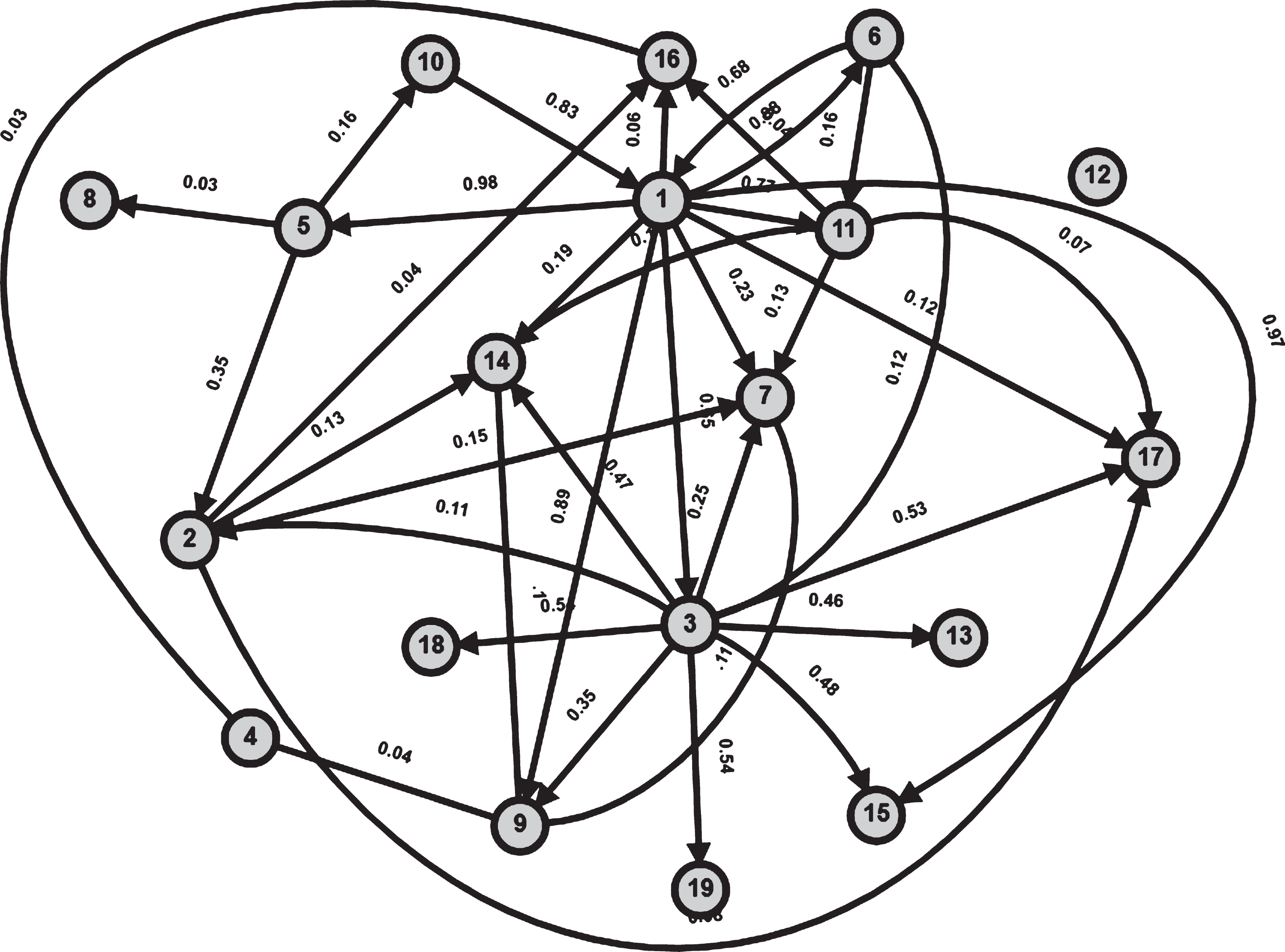
Table 5
Fuzzy mixed degree centrality of selected vertices
| Sr. No. | States (region) | Degree Centrality | Fuzzy Mixed Degree Centrality |
| 1 | Maharashtra | 10 | 1.79 |
| 2 | Tamil Nadu | 4 | 0.01 |
| 3 | Delhi | 10 | 0.58 |
| 4 | Telengana | 2 | 0.07 |
| 5 | Kerala | 3 | 0.22 |
| 6 | Rajasthan | 3 | 0.25 |
| 7 | Uttar Pradesh | 1 | –0.48 |
| 8 | Andhra Pradesh | 0 | –0.21 |
| 9 | Madhya Pradesh | 3 | –0.21 |
| 10 | Karnataka | 1 | 0.09 |
| 11 | Gujarat | 4 | –0.19 |
| 12 | Haryana | 0 | 0 |
| 13 | Jammu and Kashmir | 0 | –0.07 |
| 14 | West Bengal | 1 | –0.46 |
| 15 | Punjab | 0 | –0.1 |
| 16 | Odisha | 1 | –0.11 |
| 17 | Bihar | 0 | –0.35 |
| 18 | Uttarakhand | 0 | –0.03 |
| 19 | Assam | 0 | –0.04 |
7.1Algorithm
Calculation of fuzzy mixed degree centrality is summarized below.
Step 1: Construct a fuzzy mixed graph where both directed edges and undirected edges present in the network. For the mentioned case, the node membership values are assumed proportional to the number of affected people in the region. For this case, the membership values are the normalized value of the number of affected people. The membership values for the links are assumed as per the availability of data of mutual relation between the countries. The default case of the link membership values is the minimum of end vertex membership values.
Step 2: Adjacency numbers are calculated for each edge. Then fuzzy mixed degree centrality of any vertex is the sum of all the adjacency numbers of all adjacent edges (directed and undirected). Alternatively, the fuzzy mixed degree centrality is calculated by the following formula.
Notations have their usual meanings.
7.2Result and comparative analysis
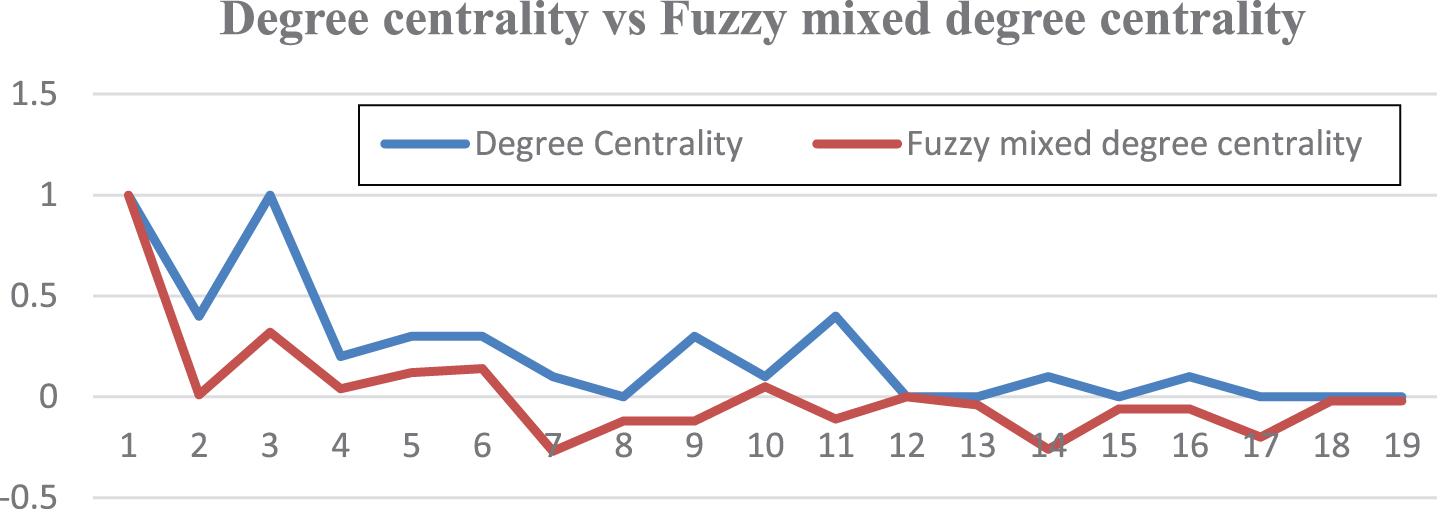
In Fig. 7, it is seen that the fuzzy mixed degree may be negative. The values are normalized in this case. Thus the values range between –1 to +1. Higher the values indicate higher the chances to spread COVID19 to others. Similarly, lower fuzzy mixed degree centrality indicates fewer chances to spread the COVID19 to other states. Along with this, degree centrality is shown. For node 1, both the centrality indicates the same. For node 3, the degree centrality is high, but the fuzzy mixed degree centrality is low. This is because the crisp data do not represent the amount of connectedness.
Fig. 7
Comparision of degree centrality and fuzzy mixed degree centrality (on the normalized data).
8Conclusions
This study captured the notion of ‘measure of directedness’ for the first time in the literature. This is the main advantage of this study from previous. How fast the information can be transferred is deduced from this measure of directedness. Several basic properties have been developed. These theories are the backbone of a new branch of fuzzy graph theory, namely as fuzzy mixed graph theory.
Thus this study will be very helpful for future research to introduce the most of fuzzy mixed graph theory topics, i.e. interval-valued fuzzy mixed graphs, generalized fuzzy mixed graphs, fuzzy mixed planar graphs etc. and applicable in many real problems in science and engineering.
References
[1] | Lambin N.V. and Tanaev V.S. , On a circuit-free orientation of mixed graphs, Dokladi Akademii Navuk BSSR 14: ((1970) ), 780–781. |
[2] | Sotskov Y.N. and Tanaev V.S. , A chromatic polynomial of a mixed graph, Vestsi Akademii Navuk BSSR Seryya Fizika-Matematychnykh Navuk 6: ((1976) ), 20–23. |
[3] | Liu J. and Li X. , Hermitian-adjacency matrices and Hermitian energies of mixed graphs, Linear Algebra Appl 466: ((2015) ), 182–207. |
[4] | Adiga C. , Rakshith B.R. and So W. , On the mixed adjacency matrix of a mixed graph, Linear Algebra and its Applications 495: ((2016) ), 223–241. |
[5] | Mohammed A.M. , Mixed Graph Representation and Mixed Graph Isomorphism, Journal of Science 30: (1) ((2017) ), 303–310. |
[6] | Yang C. and Lee Y. , Interactants and activities on Facebook, Instagram, and Twitter: Associations between social media use and social adjustment to college, Applied Developmental Science 24: (1) ((2020) ), 62–78. |
[7] | Samanta S. , Muhiudin G. , Alanazi A.M. and Das K. , A mathematical approach on representations of competitions: Competition cluster hypergraphs, Mathematical Problems in Engineering (2020), https://doi.org/10.1155/2020/2517415. |
[8] | Zadeh L.A. , Fuzzy sets, Information Control 8: ((1965) ), 338–353. |
[9] | Zadeh L.A. , Similarity relations and fuzzy orderings, Information Sciences 3: (2) ((1971) ), 177–200. |
[10] | Kauffman A. , Introduction a laTheorie des Sous-emsembles Flous, Paris: Masson et Cie Editeurs, (1973). |
[11] | Rosenfeld A. , Fuzzy graphs, Fuzzy Sets and their Applications (L.A. Zadeh, K.S. Fu, M. Shimura, Eds.), Academic Press, New York, ((1975) ), 77–95. |
[12] | Mordeson J.N. and Peng C.S. , Operations on fuzzy graphs, Information Sciences 79: ((1994) ), 159–170. |
[13] | Mordeson J.N. and Nair P.S. , Successor and source of (fuzzy) finite state machines and (fuzzy) directed graphs, Information Sciences 95: (1-2) ((1996) ), 113–124. |
[14] | Bhutani K.R. , On automorphism of fuzzy graphs, Pattern Recognition Letter 9: ((1989) ), 159–162. |
[15] | Akram M. and Dudek W.A. , Interval valued fuzzy graphs, Computers and Mathematics with Applications 61: ((2011) ), 289–299. |
[16] | Akram M. , Bipolar fuzzy graphs, Information Sciences (2011). doi:10.1016/j.ins.2011.07.037 |
[17] | Poulik S. and Ghorai G. , Detour g-interior and g-boundary nodes in bipolar fuzzy graph with applications, Hacettepe Journal of Mathematics and Statistics 49: (1) ((2020) ), 106–119. |
[18] | Poulik S. and Ghorai G. , Certain indices of graphs under bipolar fuzzy environment with applications, Soft Computing 24: (7) ((2020) ), 5119–5131. |
[19] | Sarwar M. and Akram M. , Bipolar fuzzy circuits with applications, Journal of Intrelligent and Fuzzy Systems 34: (1) ((2018) ), 547–558. |
[20] | Samanta S. and Pal M. , Fuzzy planar graphs, IEEE Transaction on Fuzzy Systems (2015). Doi: 528.10.1109/TFUZZ.2014.2387875 |
[21] | Samanta S. and Pal M. , Fuzzy k-competition graphs and p-competition fuzzy graphs, Fuzzy Information and Engineering 5: ((2013) ), 191–204. |
[22] | Samanta S. , Sarkar B. , Shin D. and Pal M. , Completeness and regularity of generalized fuzzy graphs, Springer Plus 5: ((2016) ). |
[23] | Samanta S. and Sarkar B. , Representation of competitions by generalized fuzzy graphs, International Journal of Computational Intelligence System 11: ((2018) ), 1005–1015. |
[24] | Sitara M. , Akram M. and Bhatti M.Y. , Fuzzy graph structures with applications, Mathematics 7: (1) ((2019) ), 63. |
[25] | Akram M. , Sitara M. and Saied A.M. , Residue product of fuzzy graph structures, Journal of Multiple-Valued Logic and Soft Computing 34: ((2020) ), 365–399. |
[26] | Akram M. and Sitara M. , Certain fuzzy graph structures, Journal of Applied Mathematics and Computing 61: ((2019) ), 25–56. |
[27] | Sarwar M. and Akram M. , Certain algorithms for modelling uncertain data using fuzzy tensor product Bezier surfaces, Mathematics 6: (3) ((2018) ), 42. |
[28] | Sarwar M. , Akram M. and Alshehri N.O. , A new method to decision-making with fuzzy competition hypergraphs, Symmetry 10: (9) ((2018) ), 404. |
[29] | M. Akram, M. Sarwar, and R.A. Borzooei, A novel decision making approach based on hypergraphs in intuitionistic fuzzy environment, Journal of Intelligent and Fuzzy Systems 35(2) (2018), 1905–1922. |
[30] | M. Sarwar, Decision-making approaches based on color spectrum and D-TOPSIS method under rough environment, Computational and Applied Mathematics (2020), DOI: 10.1007/s40314-020-01284-7. |
[31] | M. Sarwar, M. Akram and U. Ali, Double dominating energy of m-polar fuzzy graphs, Journal of Intelligent and Fuzzy Systems 38(2) (2020), 1997–2008. |
[32] | Akram M. , Sarwar M. and Dudek W.A. , Graphs for the analysis of bipolar fuzzy information, Studies in Fuzziness and Soft Computing, 2020, Springer, DOI10.1007/978-981-15-8756-6. |
[33] | Naseem U. , Musial K. , Eklund P. and Prasad M. , Biomedical Named-Entity Recognition by Hierarchically Fusing BioBERT Representations and Deep Contextual-Level Word-Embedding, International Joint Conference on Neural Networks (2000), 1–8. |
[34] | Naseem U. , Razzak I. , Eklund P. and Musial K. , Towards Improved Deep Contextual Embedding for the identification of Irony and Sarcasm, International Joint Conference on Neural Networks (2020), 1–7. |
[35] | Naseem U. , Razzak I. , Musial K. and Imran M. , Transformer based deep intelligent contextual embedding for twitter sentiment analysis, Future Generation Computer Systems 113: ((2020) ), 58–69. |
[36] | Khan S.K. , Farasat M. , Naseem U. and Ali F. , Performance Evaluation of Next-Generation Wireless (5G) UAV Relay, Wireless Personal Communications (2020), 1–16. |
[37] | Naseem U. , Khan S.K. , Razzak I. and Hameed I.A. , Hybrid words representation for airlines sentiment analysis, Australasian Joint Conference on Artificial Intelligence (2019), 381–392. |
[38] | Khan S.K. , Farasat M. , Naseem U. and Ali F. , Link-level Performance Modelling for Next-Generation UAV Relay with Millimetre-Wave Simultaneously in Access and Backhaul, Indian Journal of Science and Technology 12: (39) ((2019) ), 1–9. |
[39] | S.K. Khan, A. Al-Hourani, and K.G. Chavez, Performance evaluation of amplify-and-forward UAV relay in millimeter-wave, in 2020 27th International Conference on Telecommunications (ICT), 2020, pp. 1–5. |
[40] | S.K. Khan, Performance evaluation of next generation wireless UAV relay with millimeter-wave in access and backhaul, Master Thesis, School of Engineering, RMIT University, Melbourne, Australia, 2019. |
[41] | Das K. , Samanta S. and Pal M. , Study on centrality measures in social networks: A survey, Social Network Analysis and Mining 8: (13) ((2018) ), 1–11. |


