
Road detection in image by fusion laser points based on fuzzy SVM for a small ground mobile robot
Abstract
Road detection is still full of challenge for a small ground mobile robot with limited load capacity and computing resources which works in complex outdoor environment. This paper proposes a road detection method based on fuzzy support vector machine with on-line updating and retraining strategy. The algorithm extracts multi feature in image and trains a fuzzy support vector machine road classifier off-line by using few training samples. Then it detects road in laser points using a fuzzy clustering method based on maximum entropy principle. After calibrating the camera and laser range finder, and project laser points into the image, the algorithm chooses road samples with high confidence automatically according to range data and designs a rule to retraining the FSVM on-line when needed to improve its environmental adaptability. Experiments in outdoor campus environment indicate that the proposed algorithm is effective.
1Introduction
Reliable road detection is crucial to the success of many road scene understanding applications, such as unmanned ground mobile robot, autonomous driving, and driver assistance [3]. Furthermore, it can serve as a preprocessing stage for higher level reasoning and understanding of road scenes. Despite recent progress such as lots of high performance sensors have been used in this area, we are still far from having ideal solutions. Road detection remains a challenging computer vision problem due to the large variability of images acquired at different times of the day, with changing illumination, weather, different environments, and variable road conditions.
The common ground mobile robot or autonomous driving system is built on a vehicle type platform [10, 16, 17, 36]. Sensors can get relatively good field of vision on this kind of platform, which means both roadside can be seen in urban environment, so the algorithm can detect road curbs, road markings, and estimate road shape, etc. In this paper, we focus on another kind of robot platform, i.e. the small ground mobile robot as shown in Fig. 1. This is a kind of very flexible platform which makes it is suitable to complete lots of tasks, and it usually moves in structured or semi-structured road environment as its pass through ability is not strong. Compared with vehicle type platform, the small robot has to face following obvious shortcomings:
– it gets very poor visual field and can only see a very local area in front of it, which makes it is more practical to detect road surface than detect road curb for it.
– it is impossible for it to carry lots of high performance sensors as the load capacity and computing resources are very restricted in this kind of platform.
Under this circumstance, the small robot almost cannot see road curbs, so finding where does road locates is crucial for it in order to ensure its safety when moving on the road. It usually carries fewer vision sensors, typically including a low coast camera and a small laser range finder. According to this kind of sensor configuration, we present a practical road detection algorithm based on fuzzy theory in this paper. It extracts color, texture and gradient in image and train a road classifier off-line based on fuzzy SVM model at first, and then the algorithm uses a fuzzy clustering method to find road points in laser range finder data and maps road points into image after extrinsic calibrating of the camera and laser range finder. The algorithm selects road samples with high confidence (higher fuzzy membership) to replace low confidence samples in training set and retrain the FSVM classifier on-line when necessary.
The main contribution of the proposed algorithm is that we use high confidence laser detection result to guide reliable road samples chosen in image automatically and to retrain the FSVM on-line when needed to make the algorithm get high adaptability. So it is an off-line and on-line learning based algorithm, and for the on-line learning part, the algorithm can select and update reliable training samples by itself. This algorithm is mainly depending on on-line learning, which means we can use few samples to do the off-line learning. Actually, we only select samples in the first frame to do the off-line training in our experiment and this can be very clear to improve the training efficiency. We introduce fuzzy theory into the algorithm in order to improve its capability of anti-noise.
The organization of this paper is as follows: in Section 2, we summarize some related robot systems and road detection methods; Section 3 shows how to extract multi image feature to train a road classifier based on FSVM; the sample updating and classifier retraining rules is introduced in Section 4; our experiments and results are presented in Section 5; we finish the paper in Section 6 with a brief analysis of the proposed method and introducing our future work.
2Related works
Road detection for unmanned ground mobile robot has been researched in the past two decades. The earlier systems only use camera to detect road in gray or colored image, such as NAVLAB [12], VaMP [33], ARGO GOLD [1], etc., then lots of other sensors like radar or lidar have been used to deal with this problem with the development of sensor technology. Table 1 shows some typical systems that detecting road based on sensor fusion.
As far as we know, there is no universal road detection algorithm until now. Researchers usually develop their own road detection system to meet the needs of a specific application, so there are lots of road detection methods. More than one classification criteria can be used to categorize these methods. For one hand, according to sensors being used, road detection method can be categorized into camera-based [1, 4, 6, 7, 12, 14, 15, 21–23, 25, 27, 31, 33, 37– 39, 43, 46], Lidar-based [2, 9, 20, 28, 35, 47, 45], and fusion-based [11, 19, 26, 32, 40– 42]. From the beginning, the camera was used for road detection [1, 12, 21, 33], and has been extended to nowadays [6, 7, 14, 15, 22, 23, 25, 27, 31, 36– 39, 43, 46]. One can extracts road feature in image to train a classifier, but the detection results may be unstable in variable illumination, textureless, or cluttered scenes. With the development of laser measurement technology, researchers find it is easier to detect road in range data than in image and Lidar-based methods can achieve reliable and accurate results in their valid range. But range sensor usually takes low resolution and small visual field compare to camera. References [11, 19, 26, 32, 40– 42] fuse different kind of sensors to improve adaptability and robustness of the detection algorithms. Depth camera like Kinect is also used for indoor robot to detect object [40, 42] in recent years, but this kind of sensor is still not suitable for outdoor working.
For another hand, road detection methods can also be categorized into feature-based [15, 18, 19, 42], model-based [25, 44, 46] and region-based [11, 19]. Feature-based method extract road features such as color, texture, boundary, etc. to detect road, and it usually get high accuracy. But it requires the road has distinct feature identification and is sensitive to outliers. Model-based method is based on the assumption of the road model and matches the road template and image to find road. This method gets high robustness when the road model is good, but the shape of road is ever-changing in real world which makes it is very hard to build a universal road model. Region-based methods try to segment the image with road and non road area by training a classifier using multi-feature. For semi-structured or unstructured road in complex outdoor environment, region-based method usually has strong adaptability. In this paper, we focus on how to detect road by using a low cost camera and a small range finder based on image segmentation.
Road detection methods based on image feature are more easily affected by changing environmental factors such as illumination, so nowadays researchers either add prior knowledge such as road shape, or fuse camera with other kind of sensors such as lidar or IR camera, etc. At the same time, existing algorithms which use laser data are usually based on dense point cloud, especially since some high definition Lidar systems have been developed recent years. Dense point cloud contains abundant geometric information which can be used to extract more road feature or build road model, but it is also need great consumption of computing resources.
Comparing our small mobile system to vehicle platform based robot, we get poor visual field, weak performance sensors, and low computational power, so we believe that a method colligates sensor fusion, machine learning and region-based is a good way to solve our problem.
3Off-line training of FSVM
Detecting road from image can be considered as an image segmentation problem. We segment image into road area and non road area according to road color, road texture and road boundary. Generally speaking, road has different color from other area in semi-structured environment like campus or urban. The color of road usually bias blue, and gets greater brightness than non road area. Because of influenced by plants and soil, the color of non road area usually bias red and green. Texture is an expression of the intrinsic properties of the surface of the object. Texture generally exists in nature, such as fingerprints, water, wood etc., and the road texture is showed as the change of pixel gray or color. Road boundary is also an important feature as it limits the road area.
Based on the above analysis, we use color, texture and boundary as road feature in this paper and employ a FSVM model to train a classifier off-line with three main steps which are feature extraction, fuzzy SVM training and refinement. The detail of each step is expressed as follows:
3.1Image feature extraction
We extract color, texture and gradient as image feature to train a classifier. The algorithm splits an image into patches with size of 16×16 pixels at first, and then extracts each patch’s feature:
– Color
R, G and B color components are highly correlated in RGB model, so we cannot distinguish two colors based on their RGB color distance. In contrast with RGB, HSI has three independent components as shown in Fig. 2. It separates intensity out of hue and saturation, so H and S components are less influenced by the change of illumination. Based on this, we use HSI color model in this paper and calculate the average HSI color value of pixels in one patch as that patch’s color.
– Texture
We compute four kinds of Gray-level co-occurrence matrix (GLCM) as texture of road:
Angular second moment: ASM reflects the uniformity of the gray level distribution of the image. When the distribution of gray level is uniform, the elements are concentrated in the main diagonal of the GLCM, and the ASM value is large, which means the texture is uniformly distributed.
(1)
Contrast: Contrast reflects the clarity of image texture. The distance from the diagonal of GLCM is large when the texture with strong contrast.
(2)
Correlation: Correlation reflects the correlation of regional gray value. The distribution of the elements is more uniform and equal in GLCM with higher correlation.
(3)
Entropy: Entropy reflects quantity of information of the image. The GLCM and entropy is zero without texture. If one image contains rich texture information, each patch’s entropy is approximately equal which means the entropy is large. If the differences among patches are large, then the entropy is small.
(4)
We compress the gray level of the image into 16. The algorithm computes texture of four directions{0°, 45°, 90°, 135°} to eliminate the effect of direction of texture and take the average value of four direction as the texture feature.
– Gradient
We compute the gradient of each pixel according to its four neighbor pixels in a patch and take the average gradient of pixels in a patch as the patch’s gradient g.
The feature vector is expressed as Equation (5) after feature extracting.
(5)
3.2Training of FSVM
The algorithm employs a FSVM [8] to train the road classifier. FSVM can solve data set with noise better than traditional SVM. Our robot carries a low cost camera with low resolution and image quality, so FSVM is suitable for processing such images.
Each sample has a fuzzy membership in FSVM which indicates how much the sample belongs to a certain class. Value of membership decides the contribution to the decision function of one training sample. By introducing membership, the FSVM can decrease the effect of samples with noise to the trained classifier. Suppose the training samples are expressed as:
(6)
(7)
(8)
(9)
(10)
(11)
x c represents the central of a class (road or non-road), r is radius, δ indicates a small positive constant to make sure a (s i ) >0.
The algorithm selects road and non road samples manually in image as showing in Fig. 3(a) and train the FSVM. We want to emphasize here that we use few samples to do the off-line training. More precisely, we select training samples only in the first image frame in our experiment. This obviously can greatly improve the efficiency of off-line learning, but also bring higher error rate when on-line use. So we design a rule to update training samples and retrain the classifier on-line which will be explained in Section 4. The whole algorithm is mainly depending on on-line training to get better environmental adaptability.
3.3Refinement of road detection result
We use relatively small samples to train the FSVM in order to get high efficiency, and we find there are lots of wrong classified patches after initial classification (see Fig. 3(b)). So the algorithm uses following rules to refine the initial result:
– take a 8×8 template to do morphological filtering to the result image to eliminate small and isolated patches in segmented binary image (see Fig. 3(c));
– road is located in the 60% of the lower part of an image and patches belong to road should be connected, so we only take the biggest area which located in the lower part of the image as road (see Fig. 3(c));
– as we use patches instead of pixels to do computation, the road boundary in binary image is jagged. The algorithm takes median filtering to smooth the boundary (see Fig. 3(d)).
We can see the result of refinement step is good by contrasting (d) and (b) of Fig. 3.
4Update training samples on-line automatically by fusion laser points
As laser range finder gets high ranging accuracy, so we use road information detected in laser points to help us choosing high confidence road samples in image to improve the on-line performance of the algorithm. We detect road in laser points and register the range finder and camera to project laser points into the image at first, and then, reliable road samples are chosen according to pixels projected by laser points which are dart on road. The FSVM will be retrained using these road samples if needed.
4.1Road detection in laser points
Laser points are collected by a UTM-30LX laser range finder. The range finder takes an inclined angle when installing in order to “look on” the road. We employ a fuzzy clustering algorithm based on Maximum Entropy Principle (MEP) [44] to cluster laser points in a data frame and find points which are located on road.
It is assumed the threshold of prediction error is δ, the next predicted laser point’s position is
(12)
The point will be considered to be the start of another cluster if e i > δ. The parameter δ should be determined according to the distance between range finder and the target. We use Equation (2) to compute δ.
(13)
Parameter a in Equation (13) is a scale factor to counteract noise. Parameter θ is half of angular resolution of azimuth of UTM-30LX. (x t , y t ) is the coordinate of a point p i .
Suppose every frame of range data gets N points and the system model can be characterized by M cluster centers
There will be a prediction error at each time when predict the position of the next point, and the accumulated error problem is on the table if we ignore this error. In our algorithm, each vector in input vector
(14)
(15)
For data point measured at time t, the probability of it belongs to the cluster centers can be viewed as its fuzzy membership μ i , where μ i ∈ [0, 1] and i = 1, 2, . . . , M. The summation of all μ i ’s is equal to one. The clustering process can be formulated as an optimization problem and the corresponding cost function to be minimized is defined as:
(16)
The distribution of μ i is unknown in our problem. According to the information theory, the MEP is the most unbiased prescription to choose the values of the membership, μ i , for which Shannon entropy, i.e., the expression
(17)
(18)
The final solved probabilities are of the Gibbs distribution [30, 29], i.e.
(19)
Take Equation (20) into Equation (16), and versus λ differentiate, and then take the experiential parameter [29] we get:
(20)
Weighting reasoning mechanism is used to compute the output vector as our system present a linear trend. The following formula will account for that trend well.
(21)
(22)
Hereto, we have introduced the clustering step. It does not require training which enables it to work on-line completely.
The ideal road model is shown in Fig. 4, but usually we cannot see the both side of the road because of occlusion. So it is unreliable to detect left and right curb in one laser frame data to find the road. Fortunately, the road in campus and urban is usually flat, so laser points dart on road satisfies linear distribution. We do linear fitting of each cluster of points and take clusters with small linear fitting mean square error as the candidate road cluster. There are lots of linear distributed point clusters are not belong to road obviously as any sample points from regular surface are linear distributed. We have to design some filters to find real road in range data.
We known the angle of yaw, roll and pitch of the robot by using a gyro and we transform points to the robot coordinates O R , The road surface around the robot should be horizontal in O R so we search horizontal linear distributed clusters of points after project them into ground plane. Suppose the included angle between the horizontal and a linear distributed cluster r i is β and the average height of points in r i is h r i , the height of the robot located is h R . The length of r i is L and the least width that the robot can be passed through is W. Then the first three road filters are expressed in Equation (23). Δβ is the threshold of the error of horizontal and h is the highest height of road surface. Δh is the threshold of the height differences between the robot current located area and the front road area.
(23)
(24)
(25)
Equation (23) is used to analyze the single data frame of range finder. Points in one frame are sparse, so we use the temporal and spatial correlation in the process of robot motion to increase the confidence of road detection. The height of the road should be consistent in a local area, and here will be obstacle exist if situation shown in Fig. 5 appeared. We use Equation (24) to limit the change of the road height at adjacent moment.
At last, clusters of points r i satisfy Equation (25) will be chosen as road. Figure 6 shows the road detection result in laser points. Road detected by range data usually get higher confidence than that detected in image so we use this information to help find reliable road samples in image automatically.
4.2Registration of the ranger finder and camera
The calibration of the camera and laser range finder is shown in Fig. 7(a) and we use the method proposed in [34] to solve this extrinsic calibration problem. Laser points can be mapped onto the image after calibration as shown in Figs. 7(b) and 7(c).
4.3Updating training samples on-line
We use only 200 training samples in order to improve training efficiency which will inevitably leads to the classification error become higher and higher along with the robot’s movement and the change of environment. So we design the rule to update the training samples on-line to improve the adaptability of the proposed algorithm.
The algorithm takes the patches in image under the mapped road line after projecting road laser points onto the image (shown in Fig. 7) as road samples with high confidence. This is reasonable because the field of vision of camera mounted on our robot is very low. Figure 8 shows an ideal situation without obstacles on road. The laser point dart on road projected onto image will become multi-line with obstacle and the algorithm only take patches under road lines as the road samples under this condition. The algorithm uses the upper left and upper right area as the high confidence non-road samples.
According to the on-line estimated classification error computed the algorithm decides when to update samples and retraining the FSVM. It takes the coarse segmentation image subtraction the corresponding refined one to get error classified patches S road and S non - road and who will be chosen as updating samples C road and C non - road if they satisfy following constraints: (1) S road and S non - road are not locate on around the boundary between road and non-road area in image as the boundary may not clearly enough to be choose as high confidence samples (gray area in Fig. 2(e)); (2) The area of S road and S non - road should be big enough. These tow constraints can be expressed as:
(26)
(27)
So far, we have introduced out road detection method. We summarized the proposed algorithm as the flow chart shown in Fig. 9.
5Experiments
We use the robot platform shown in Fig. 1 to collect experimental data in real outdoor campus environment. This robot is a very small ground mobile platform with size of 0.36 m (L)×0.35 m (W)×0.45 m (H), and equips a small DAHENG Mercury camera, a HOKUYO UTM-30LX laser range finder, a IG-500 N GPS aided AHRS and odometer.
Fig. 10 shows some experiment result: Original pictures of the scene with extracted road boundary are shown in Figure 10(a). Result of road detection by SVM and the proposed method based on FSVM are shown in Figs. 10(b) and 10(c) respectively. Figure 10(d) shows the final result. We can see that Fig. 10(c) got better result than Fig. 10(b), which means the proposed method has stronger environment adaptability. Updating and retraining FSVM can deal with factors of environmental changing.
We test the algorithm by using continuous frames while the robot moving in campus. Figures 11(a) and 11(b) shows original image and result of road detection in 8 continuous frames. There exist an intersection, shadow and changing illumination in these 8 frames during the robot moving. Road detection result shows the proposed algorithm has the ability to deal with these changing environment factors.
Figures 11(c) and 11(d) are error rate of detection results of 100 frames by using FSVM and SVM respectively. The lateral axis indicates number of frames and vertical axis indicates detection error rate of one frame. Suppose N is the total number of patches in one image, and N err is the difference number of patches between FSVN or SVM classification result and manual labeled ground truth, then the error rate is defined as r err = N err /N. We can see the average classification error rate of FSVM is 6.3% , which is better than 8.5% gotten by SVM. We give full consideration to the samples for each category of membership degree when use FSVM, so the error rate is low at the first frame in (c) compared to (d). And the error rate is relatively stable in continuous detection of 100 frames. Thus the proposed algorithm is not only improves the accuracy of classification, but also can better adapting to environmental changes.
The effect of refinement and the comparison between without and with on-line training is tested. Form Fig. 12(b) we can see that the sky is easily classified as the road without refinement, and the results are improved a lot after refinement as shown in Fig. 12(c). Road detection results are further improved when on-line learning is used by comparing Figs. 12(d) and (c).
Previous experimental results show the algorithm has good environmental adaptability to deal with road scenes. In urban environment, obstacles are one of the factors that affect road detection result, so we test the proposed algorithm in campus when there are different obstacles on road. Figure 13 shows typical detection results, and we can see all obstacles that on road are detected. We know that color and texture of obstacles in urban environment usually different from the road, so it is not very hard for the proposed algorithm to recognize obstacles theoretically, and experiments in real environments also validate this according Fig. 13.
6Conclusion
Road detection is still full of challenge, especially for a small ground mobile robot with limited load capacity and computing resource who works in complex outdoor environment. In this paper we present a road detection method based on fuzzy theory. It extracts multi image feature and trains a FSVM classifier with few training samples off-line to get higher training efficiency. Then an on-line training sample updating and retraining strategy is used to make the algorithm has strong adaptability to adapt dynamic outdoor environment. As we use low performance sensors, we introduce fuzzy theory in our algorithm to improve its anti-noise capability. Experiments in the real campus environment validate the method.
Our future research will focus on tilting the laser range finder to get a range image and use this kind of data to navigate the outdoor mobile robot. We have built a tilting system and registered multi-frame laser data in static state already, but it is hard to get high-accuracy range image when the robot moves on rugged ground because of the big random shaking. We will try our best to deal with this problem and design a small and high-performance outdoor environmental detection and understanding system for intelligent ground mobile robot.
Acknowledgments
This work was supported by the Natural Science Foundation of Jiangsu Province of China under Grant No. BK2012399, the doctoral program of higher education of specialized research fund of China under Grant No. 20123219120028, the Key Laboratory of Intelligent Perception and Systems for High-Dimensional Information (Nanjing University of Science and Technology), Ministry of Education under Grant No. 30920140122006 and the Fundamental Research Funds for the Central Universities under Grant No. 30915011321.
References
1 | Broggi A, Pavia U, Bertozzi M, Fasciol A (1999) ARGO and the MilleMiglia in automatic tour Intelligent Systems and their Applications 14: 55 64 |
2 | Hervieu A, Soheilian B (2013) Road side detection and reconstruction using LIDAR sensor In Proceedings of the IEEE on the Intelligent Vehicles Symposium, Gold Coast 1247 1252 |
3 | Geiger A, Lenz P, Urtasun R (2012) Are we ready for autonomous driving? The kitti vision benchmark suite RI, USA CVPR, Providence |
4 | Seibert A, Hahnel M, Tewes A, Rojas R (2013) Camera based detection and classification of soft shoulders, curbs and guardrails IEEE Intelligent Vehicles Symposium, Gold Coast 853 858 |
5 | Kim BS, Xu SL, Savarese S (2013) Accurate localization of 3D objects from RGB-D data using segmentation hypotheses, IEEE Conference on Computer Vision and Pattern Recognition 3182 3189 Oregon, USA |
6 | Wang B, Fremont V (2013) Fast road detection from color images IEEE Intelligent Vehicles Symposium (IV) 1209 1214 Gold Coast City, Australia |
7 | Wang B, Fremont V, Rodriguez SA (2014) Color-based road detection and its evaluation on the KITTI road benchmark,IEEE Intelligent Vehicles Symposium Proceedings 31 36 Dearborn, Michigan, USA |
8 | Lin CF, Wang SD (2002) Fussy support vector machine IEEE Trans. on Neural Networks 13: 464 471 |
9 | Habermann D, Carcia C (2010) Obstacle detection and tracking using laser 2D Latin American Robotics Symposium and Intelligent Robotic Meeting (LARS), Sao Bernardo do Campo 120 125 Brazil |
10 | Hong D, Kimmel S, Boehling R (2008) Development of a semi-autonomous vehicle by the visually-impaired IEEE International Conference on Multisensot fusion and Integration for Intelligent Systems 539 544 Seoul |
11 | Maier D, Bennewitz M, Stachniss C (2011) Self-supervised obstacle detection for humanoid navigation using monocular vision and sparse laser data, IEEE International Conference on Robotics and Automation 1263 1269 Beijing, China |
12 | F. Dellaert, D. Pomerlau and C. Thorpe, Model-based car tracking integrated with a road-follower, IEEE International Conference on Robotics and Automation, Leuven, 1998, pp. 1889–1894, On Intelligent Vehicles Symposium, Tokyo, 1996, pp. 391–396. |
13 | Arbeiter G, Fuchs S, Hampp J, Bormann R (2014) Efficient segmentation and surface classification of range images IEEE International Conference on Robotics and Automation 5502 5509 Hong Kong, China |
14 | Vitor GB, Victorino AC, Ferreira JV (2014) A histogram-based joint boosting classification for determining urban road, IEEE International Conference on Intelligent Transportation Systems (ITSC) 2245 2246 Qingdao, China |
15 | Vitor GB, Lima DA, Victorino AC, Ferreira JV (2013) A 2D/3D vision based approach applied to road detection in urban environments IEEE Intelligent Vehicles Symposium (IV) 952 957 Gold Coast City, Australia |
16 | Chris U (2009) The urban challenge, International Conference on Information Fusion 1 10 Seattle, Washington, USA |
17 | Stanek G, Langer D, Muller-Bessler B, Huhnke B (2010) Junior 3: A test platform for advanced driver assistance systems IEEE Conference on Intelligent Vehicles Symposium 143 149 San Diego |
18 | Zhang G, Zheng NN, Cui C, Yan YZ (2009) An efficient road detection method in noisy urban environment IEEE Intelligent Vehicles Symposium 556 561 Xi’an, China |
19 | Zhang HH, Wang JL, Fang T, Quan L (2014) Joint segmentation of images and scanned point cloud in large-scale street scenes with low-annotation cost IEEE Transactions on Image Processing 23: 4763 4772 |
20 | Guan HY, Li J, Yu YT, Chapman M, Wang C (2015) Automated road information extraction from mobile laser scanning data IEEE Transactions on Intelligent Transportation Systems 16: 194 205 |
21 | Ulrich I, Nourbakhsh I (2000) Appearance-based obstacle detection with monocular color vision 866 871 Austin, Texas, USA AAAI |
22 | Alvarez JM, Lopez AM, Gevers T, Lumbreras F (2014) Combining priors, appearance, and context for road detection IEEE Transactions on Intelligent Transportation Systems 15: 1168 1178 |
23 | Alvarez JM, Salzmann M, Barnes N (2014) Data-driven road detection, IEEE Winter Conference on Applications of Computer Vision (WACV), Steamboat Springs 1134 1141 CO, USA |
24 | Alvarez JM, Gevers T, Lopez AM (2009) Vision-based road detection using road models, IEEE International Conference on Image Processing 2073 2076 Cairo, Egypt |
25 | Alvarez JM, Gevers T, Diego F, Lopez AM (2013) Road geometry classification by adaptive shape models IEEE Transactions on Intelligent Transportation Systems 14: 459 468 |
26 | Tan J, Li J, An XJ, He HG (2014) Robust curb detection with fusion of 3D-lidar and camera data Sensors 14: 9046 9073 |
27 | Lu K, Li J, An XJ, He HG (2014) A hierarchical approach for road detection IEEE International Conference on Robotics and Automation (ICRA) 517 522 Hong Kong, China |
28 | Yeonsik K, Chiwon R, Seung-Beum S, Bongsob S (2012) A lidar-based decision-making method for road boundary detection using multiple Kalman filters IEEE Trans Ind Electron 59: 4360 4368 |
29 | Rose K (1998) Deterministic annealing for clustering, compression, classification, regressions and related optimization problems Proceedings of the IEEE 86: 2210 2239 |
30 | Rose K, Gurewitz E, Fox GC (1990) Statistical mechanics and phase transitions in clustering Phys Rev Lett 65: 945 948 |
31 | Beyeler M, Mirus F, Verl A (2014) Vision-based robust road lane detection in urban environments IEEE International Conference on Robotics and Automation (ICRA) 4920 4925 Hong Kong, China |
32 | Enzweiler M, Greiner P, Knoppel C, Franke U (2013) Towards multi-cue urban curb recognition In Proceedings of the IEEE Intelligent Vehicles Symposium 902 907 Gold Coast City, Australia |
33 | Maurer M, Dickmanns ED (1997) A system architecture for autonomous visual road vehicle guidance IEEE Conference on Intelligent Transportation System 578 583 Boston |
34 | Zhang QL, Pless R (2004) Extrinsic calibration of a camera and laser range finder (improves camera calibration), IEEE International Conference on Intelligent Robots and Systems 2301 2306 Sendai, Japan |
35 | Matthaei R, Lichte B, Maurer M (2013) Robust grid-based road detection for ADAS and autonomous vehicles in urban environments, International Conference on Information Fusion (FUSION) 938 944 Istanbul, Turkey |
36 | Tedrake R, Fallon M, Karumanchi S (2014) IEEE International Conference on Robotics and Automation A summary of team MIT’s approach to the virtual robotics challenge 2087 Hong Kong |
37 | Zhou SY, Gong JW, Xiong GM, Chen HY (2010) Road detection using support vector machine based on-line learning and evaluation IEEE Intelligent Vehicles Symposium (IV) 21: 256 261 |
38 | Zhou SY, Iagnemma K (2010) Self-supervised learning method for unstructured road detection using fuzzy support vector machines, IEEE/RSJ International Conference on Intelligent Robots and Systems 1183 1189 Taipei, Taiwan |
39 | Kuhnl T, Fritsch J (2014) Visio-spatial road boundary detection for unmarked urban and rural roads, IEEE Intelligent Vehicles Symposium Proceedings 1251 1256 Dearborn, Michigan, USA |
40 | Huang WQ, Gong XJ, Liu JL (2013) Integrating visual and range data for road detection, IEEE International Conference on Image Processing (ICIP) 4136 4140 Melbourne, Australia |
41 | Huang WQ, Gong XJ, Xiang ZY (2014) Road scene segmentation via fusing camera and lidar data IEEE International Conference on Robotics anf Automation 1008 1013 Hong Kong, China |
42 | Hu X, Rodriguez FSA, Gepperth A (2014) A multi-modal system for road detection and segmentation, IEEE Intelligent Vehicles Symposium Proceedings 1365 1370 Dearborn, Michigan, USA |
43 | Liu X, Shang KK, Liu J, Zhou CY (2014) Unstructured road detection based on fuzzy clustering arithmetic, International Conference on Fuzzy Systems and Knowledge Discovery (FSKD) 114 118 Xiamen, China |
44 | Yuan X, Zhao CX (2010) Traversable area extraction using LIDAR sensor Acta Armamentarii 31: 1702 1707 |
45 | Zhong XY, Peng XF, Zhou JH (2011) Detection of moving obstacles for mobile robot using laser sensor, The 30th Chinese Control Conference 4002 4006 Yantai, China |
46 | He Z, Wu T, Xiao ZP, He HG (2013) Robust road detection from a single image using road shape prior, IEEE International Conference on Image Processing (ICIP) 2757 2761 Melbourne, Australia |
47 | Liu Z, Wang J, Liu D (2013) A new curb detection method for unmanned ground vehicles using 2D sequential laser data Sensors 13: 1102 1120 |
Figures and Tables
Fig.1
A small ground mobile robot platform with size of 0.36 m (L)×0.35 m (W)×0.45 m (H).
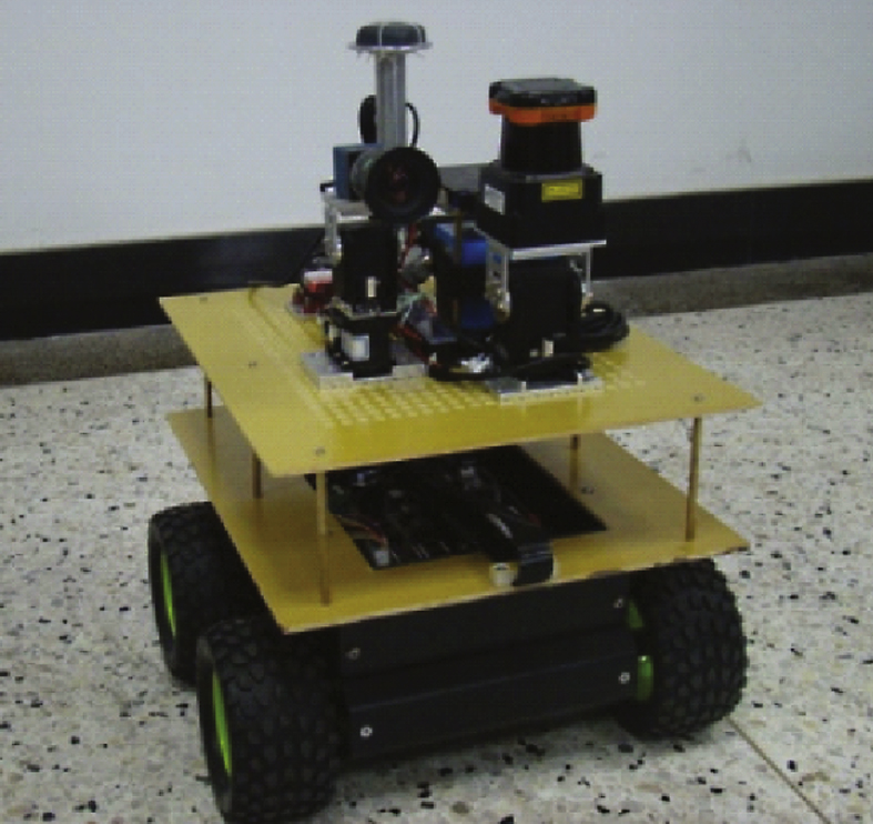
Fig.2
RGB and HSI color, (a) RGB image, (b) H component, (c) S component, (d) I component.
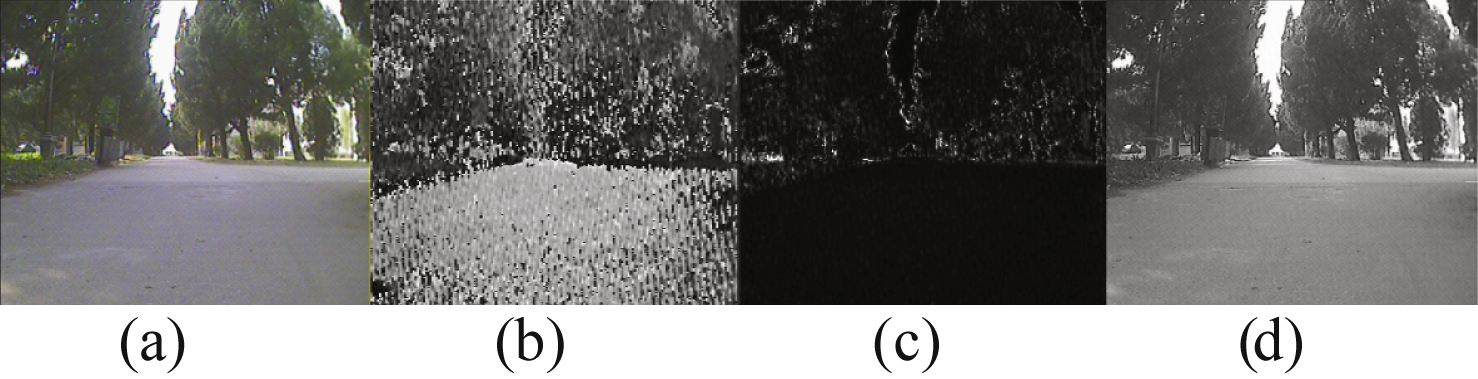
Fig.3
Road detection result in image: (a) training sample selection, (b) road detection after initial classification, (c) road detection after refine step 1and 2, (d) result after smoothing (c), (e) a demonstration of S boundary mentioned in Section 4.3.
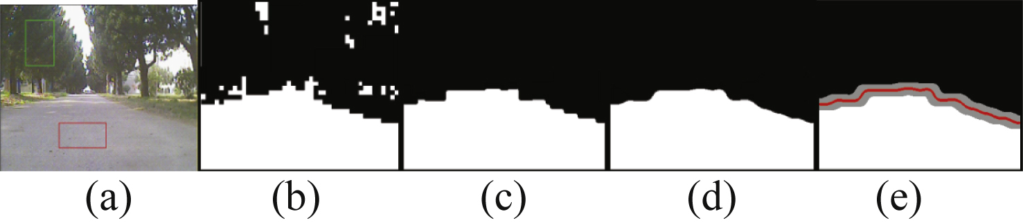
Fig.4
Ideal road model.
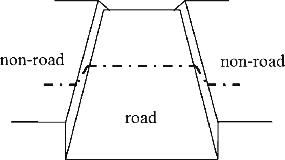
Fig.5
Change of road height between time t and t + 1.
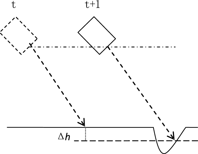
Fig.6
Road detection in laser points, (a) original scenes, (b) points clustering with red points are start or end point of a cluster, (c) results of road detection shown in red line.
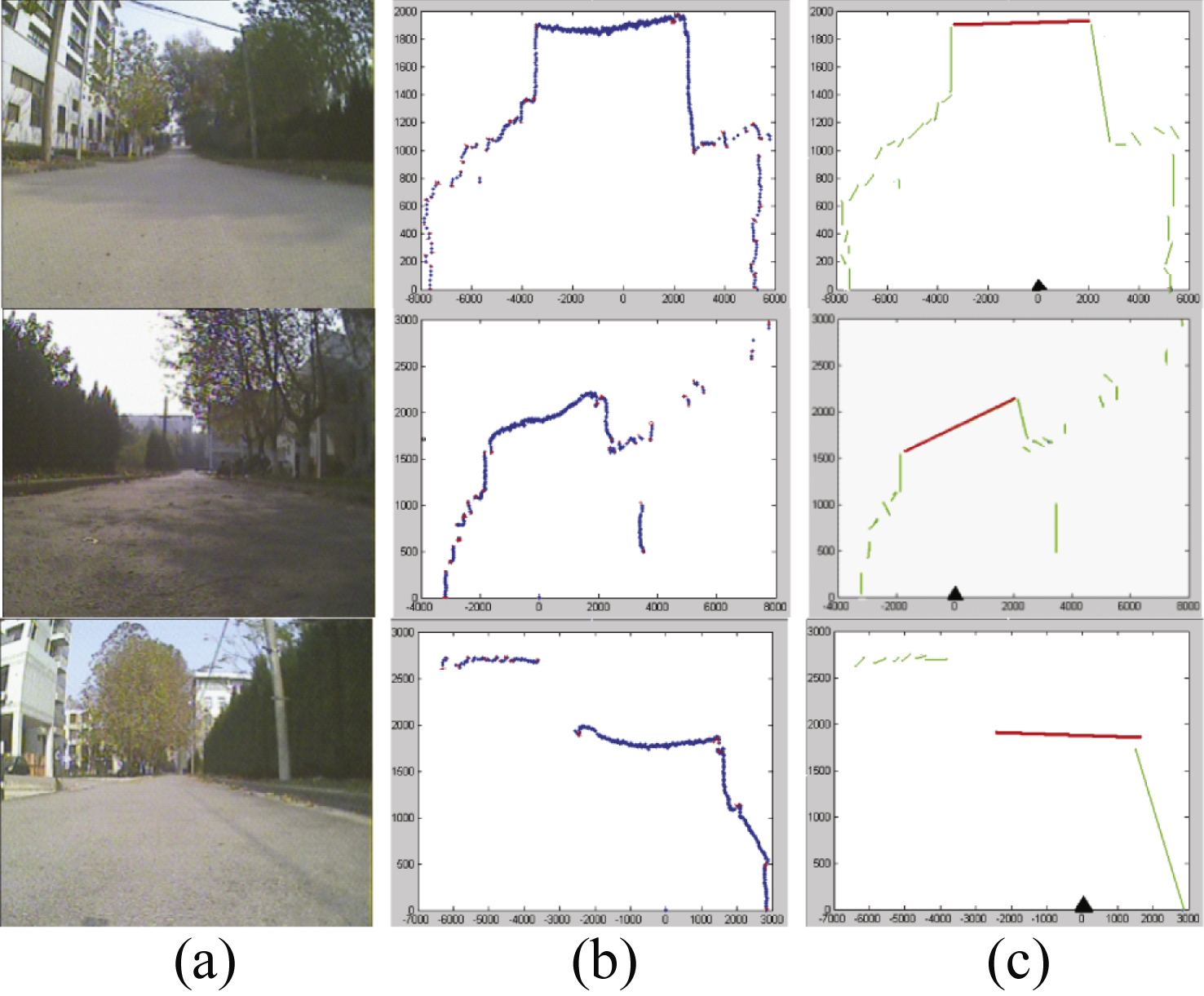
Fig.7
Registration of a camera and laser range finder Laser points. (a) the coordinate of two sensor, (b) and (c) laser points mapped into image after registration (green pixels).
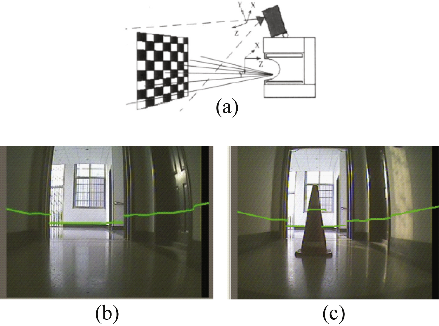
Fig.8
High confidence road area after mapping laser points into image. The red line is the road detected in laser point projected into image and white area under red line is road samples with high confidence level. The blue line is the outline of the road detected by FSVM.
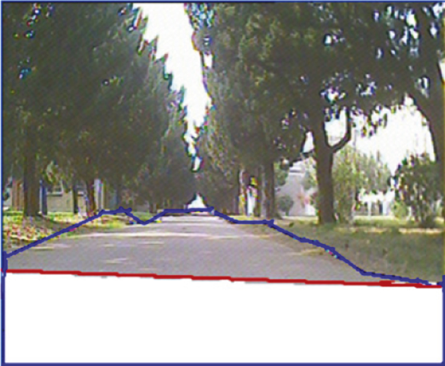
Fig.9
Flow chart of the proposed algorithm.
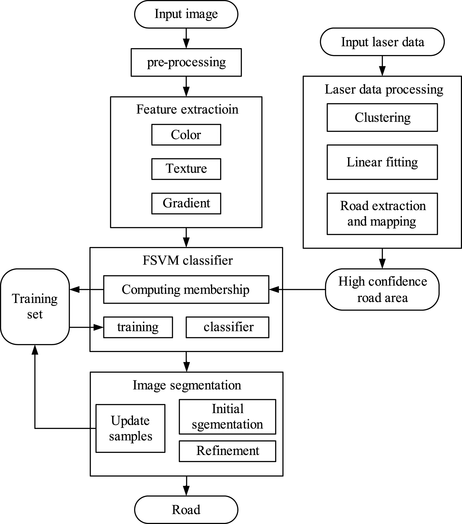
Fig.10
Results of road detection, (a) original scenes and road boundary, (b) results of SVM, (c) results of FSVM, (d) results after refinement based on (c), i.e. result of the proposed algorithm.
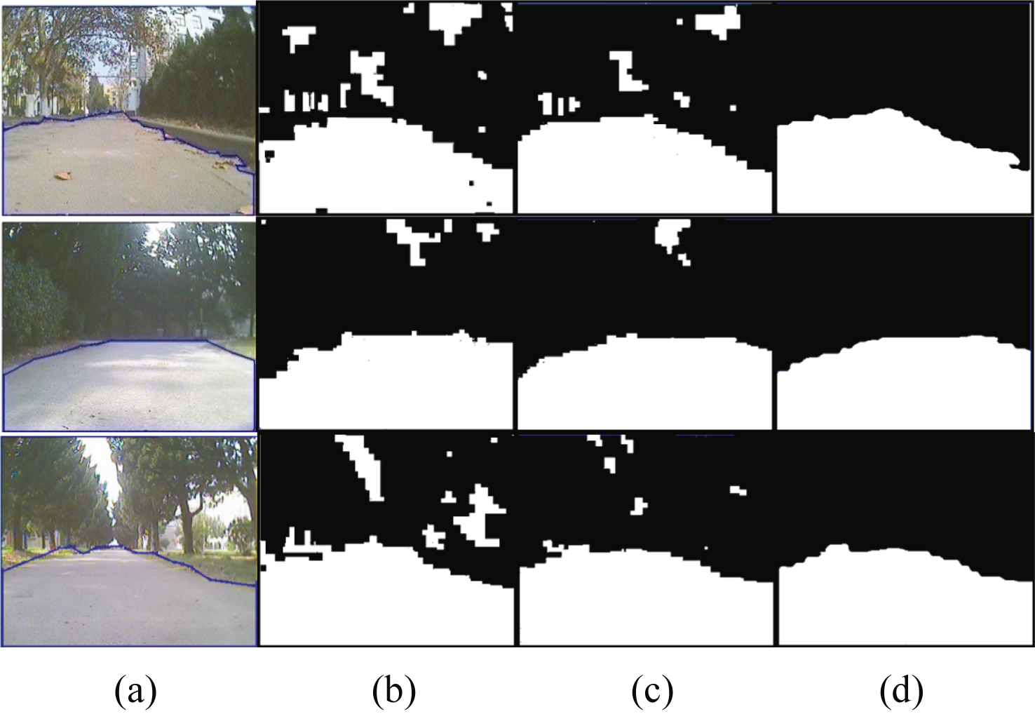
Fig.11
Results of continuous frames, (a) original scenes, (b) results of road detection, (c) error rate of FSVM, (d) error rate of SVM.
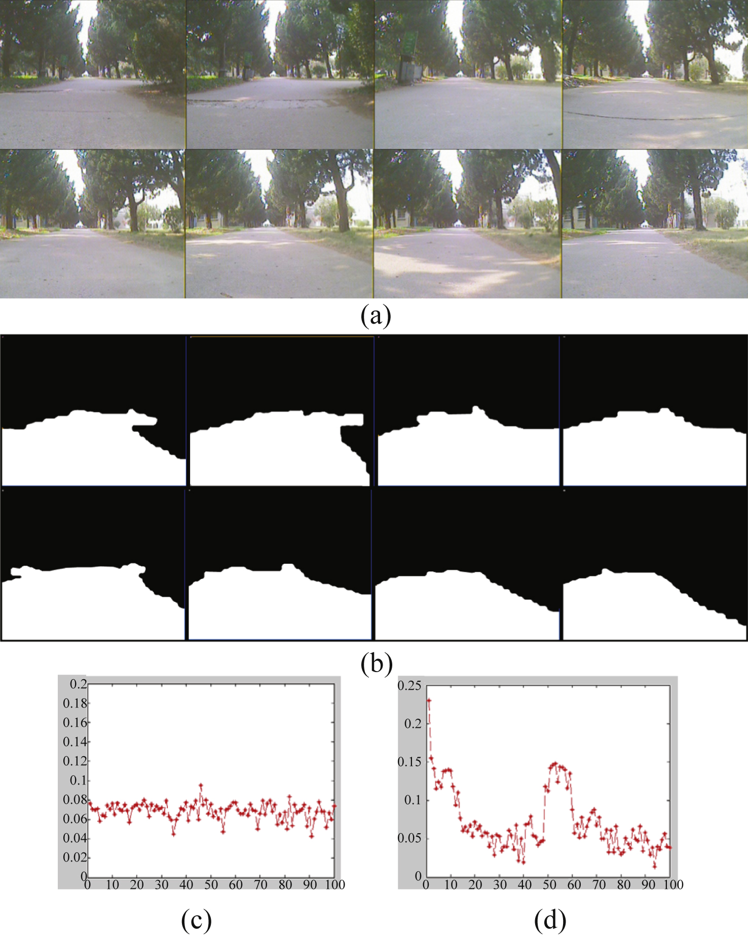
Fig.12
Comparison of results between without and with on-line training. From top to down: frame no. 21, 31, 41, 49, 61 and 89. (a) original scenes, (b) results of without on-line training and without refinement, (c) results of without on-line training after refinement, (d) results of with on-line training after refinement.
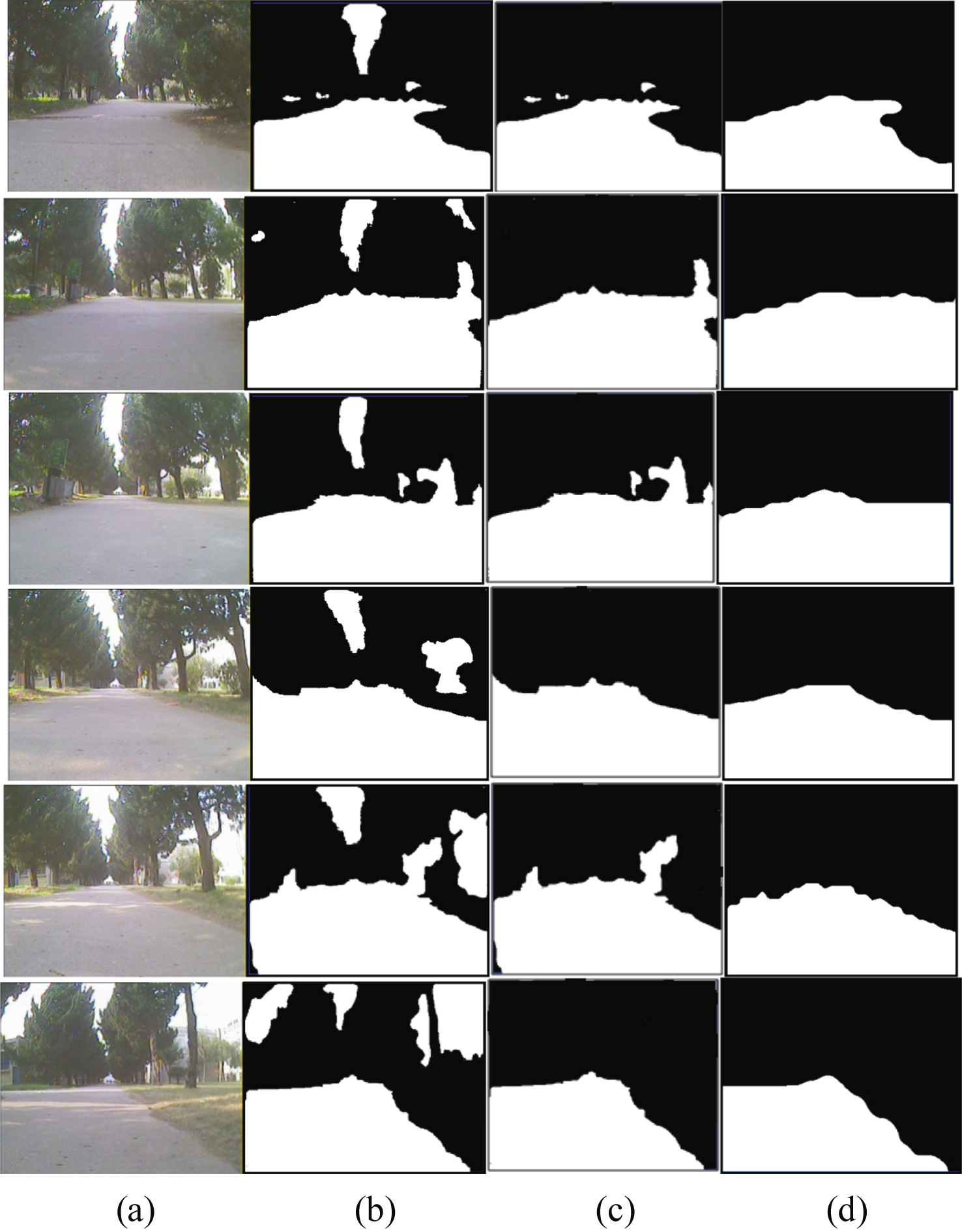
Fig.13
Result of road detection with obstacles on the road, (a) original scenes, (b) result of road detection.
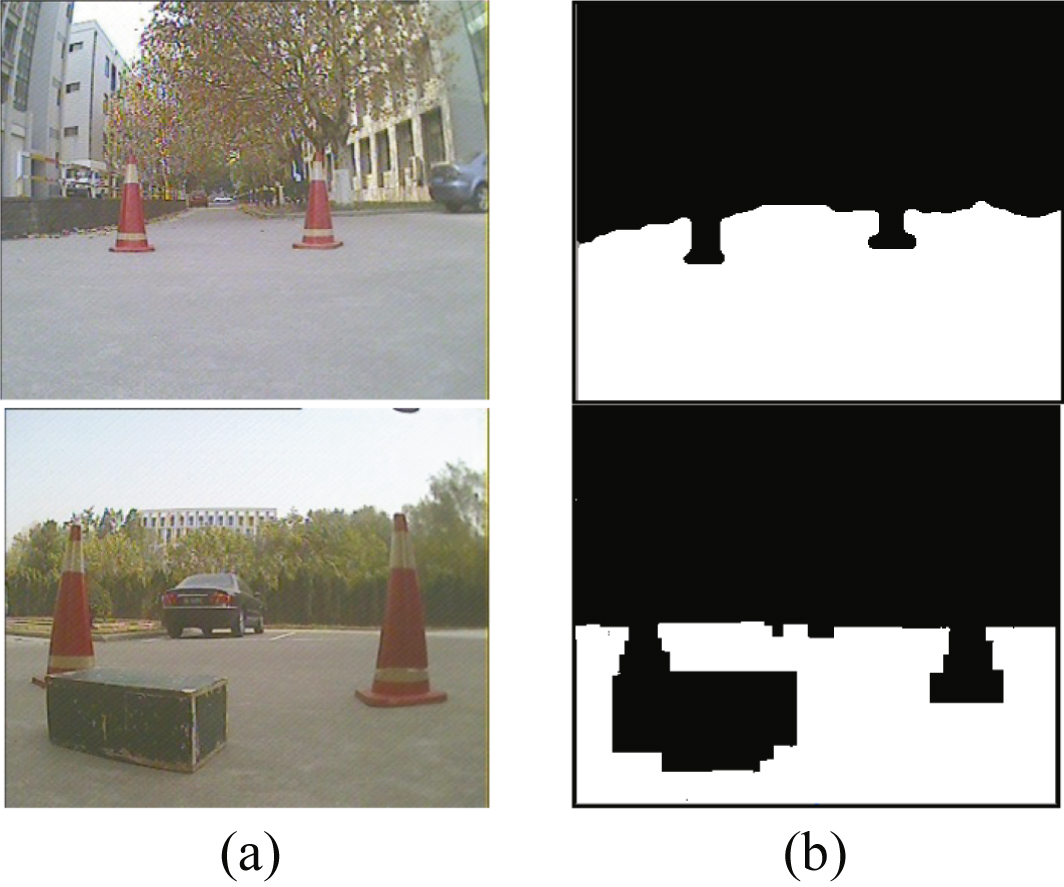
Table 1
Some typical unmanned ground vehicle systems
| System name | Year | Sensors | Adaptive environment |
| Odin [10] | 2007 | Colored camera, lidar | Outdoor nature scene |
| BOSS [16] | 2008 | Laser range finder, HDL 64E Lidar, binocular camera system | Urban |
| Junior 3 [17] | 2010 | Laser range finder,Riegl laser, HDL 64E Lidar, Bosch Radae, colored camera | Urban |
| VRC [36] | 2013 | Laser range finder, binocular camera system | Complex environment |


