
Intelligent guidance method based on differential geometric guidance command and fuzzy self-adaptive guidance law
Abstract
Differential geometric guidance command (DGGC) is widely acknowledged as a better method of endoatmospheric interception than three-dimensional (3D) pure proportional navigation (PPN). DGGC can be regarded as an intelligent method due to its sophisticated sense of Lyapunov. However, traditional DGGC cannot guarantee line of sight (LOS) finite time convergence (FTC) to zero against maneuvering targets, particularly in regard to a stable, robust trajectory, which effectively lowers the overall intelligence of the method. This study proposes employment of the fuzzy self-adaptive guidance law to estimate target acceleration and enhance guidance intelligence, which in turn enhances the intelligence of the traditional DGGC method, making it more adaptive and applicable to practical interception scenarios. Finally, the effectiveness of this newly-proposed guidance method is demonstrated by numerical simulation.
1Introduction
Missile guidance and control systems are extremely complex due to their multi-variable, non-linear nature and dependence on time variation, both of which are easily affected by environment. In recent years, missile guidance systems have largely investigated improvements in maneuverability by improving speed, acceleration, etc. However, the traditional PPN guidance law is unable to meet the increasing difficulty of interception requirements, particularly for targets that exhibit great maneuverability. Therefore, the development of a new guidance law has become a priority for military technology as time convergence and intelligence capabilities become increasing more important for anti-missile systems. While the fuzzy guidance law provides stabilization, robustness and intelligence, new adaptations are sought to strengthen terminal guidance systems [6, 18].
Proportional navigation (PN) has been widely used due to the non-maneuverability of targets in early engineering practices of the missile guidance community [14]. However, PN performance is greatly reduced against highly maneuverable targets. Much recent research has been devoted to the development of new guidance laws which aim to improve the intelligence of anti-missile systems, enabling them to handle increasingly agile targets based on modern control theories such as adaptive and H-∞ control.
The differential geometric guidance command (DGGC) is a novel guidance law, the purpose of which is to improve endoatmospheric interception of maneuvering targets. Chiou and Kuo [2, 21] initially studied the three-dimensional motion of missile and target in the arc-length system with the aid of classical differential geometry theory, and proposed DGGC in the arc-length system. C.Y. Li, et al. [3–5] translated the DGGC of the arc-length system into the time domain, and studied scenarios of DGGC interception of a tactical ballistic missile, as well as the initial capture condition of the case. K.B. Li, et al. [10–13] analyzed DGGC according to the relative kinematic equations established in the line of sight (LOS) rotation reference system, and proposed a new, simplified DGGC formation. The primary contribution of DGGC is the derivation of a new direction of command acceleration, which better controls the LOS rate compared to traditional 3D PPN. This property provides DGGC the opportunity to improve performance by combining with other guidance strategies. Ye, et al. [9] presented a modified DGGC combined with sliding mode control theory; however, this modification guarantees only the asymptotic convergence of the LOS, and requires the upper bound of the target acceleration in order to construct the guidance command. Ariff, et al. proposed a differential geometric guidance law by using the involute of the target trajectory. White, et al. [1, 15] presented another differential geometric guidance law which was thought to improve traditional PN.
For modern guidance laws designed for the interception of maneuverable targets, the finite time convergence of the LOS rate is essential. Therefore, much recent research has been devoted to investigation of this property. Haimo [19] initially proposed the finite time control law in 1986. Gurfil, et al. [16] discussed the issue of finite time stability of guidance systems. Wu, et al. [17] reported a finite time guidance law designed to intercept fixed targets based on the nonlinear three-dimensional relative kinematics of the missile and target. Zhou, et al. [7] proposed a finite time convergence guidance law specifically designed for the interception of maneuverable targets that was able to guarantee LOS rate convergence in finite time, but required knowledge of the upper bound of the target acceleration. Wang, et al. [20] proposed a partially-integrated sliding mode guidance law; however, the law was quite complex and required the use of higher order variables in the guidance command that proved difficult to measure, and had to be estimated by a sliding mode observer.
The primary cause of missed missile targets is target acceleration. Recently, a Lyapunov function based on a switching fuzzy controller has attracted much attention in the field of control systems, and has become a popular research focus [8, 22]. It has also become popular to use the fuzzy self-adaptive guidance law (FSG) to estimate target acceleration during the guidance process. Because the fuzzy control method does not require the establishment of a precise mathematical model, an estimate of the interference quantity of target acceleration and other measurements are initially obtained. Next, fuzzy control technology is applied to determine the switching coefficient, so as to weaken the chattering and robustness ofthe system.
In this paper, DGGC with FTC and FSG (DGGC-FE) is proposed to overcome the disadvantages of Zhou’s approach and improve the endoatmospheric interception of maneuverable targets. Simulation results indicate that the use of the differential geometric guidance command and the fuzzy self-adaptive guidance law enables the proposed method to enhance guidance intelligence.
This paper is organized as follows. Section 2 introduces the theory of variable universe fuzzy control. Section 3 describes the differential geometry theory and the basic components of DGGC; the finite time stabilization of nonlinear systems is briefly articulated, and a new DGGC with FTC (DGGC-F) is described. Section 4 estimates the target acceleration according to FSG, and DGGC-FE is proposed. In Section 5, the effectiveness of DGGC-FE is validated via numerical simulation. Section 6 presents conclusions based on the obtained data and simulation results.
2Variable universe fuzzy control theory
2.1Definitions of basic elements of the fuzzy control theory
In order to facilitate the mathematical description, one may consider the fuzzy set as a set of peaks.
2.2Interpolation mechanism of fuzzy control
Fuzzy control output can be assigned to the controlled object only after the solution is determined to be fuzzy. Calculation of the exact output value is a process of interpolation. The mathematical expression of the output function is expressed as follows:
(1)
where
(2)
The formula first requires an input as a fixed parameter. The other parameter is interpolated, and the parameters are then inputted together. The formula can also be regarded as a data interpolation set.
2.3Variable universe fuzzy control theory
Fuzzy control is used to achieve high-precision control, which requires an increase in the number of rules; fuzzy control is more successful when the error is large. Failure of fuzzy control is often due the inability to insert additional rules in the vicinity of zero. Therefore, the primary obstacle to the application of fuzzy control in missile guidance is a dearth of rules near a zero point. Thus, the use of a variable universe is a method by which to increase the number of rules in the vicinity of zero, and is realized by a scaling factor.
Definition 1. The function α : X → [0, 1] , X| → α (x) represents a scaling factor of the domain X, if it satisfies the following conditions:
– (∀ x ∈ X) (α (x) = α (- x));
– α (0) =0;
– α is strictly monotonic when α ∈ [0, E];
– (∀ x ∈ X) (|x| ≤ α (x) E);
– α (± |E) =1, β (± U) =1.
The scaling factor function adjusts the size of the variable universe according to the established error. Thus, α (x) =1 - λ exp(- kx 2) , λ ∈ (0, 1) , k > 0 represents an input signal scaling factor, and β (u) = K|e/E| τ3|ec/EC| τ4 represents an output signal scaling factor.
3Basic control theory of missile-target engagement and the guidance command with finite time convergence
The flight trajectories of an endoatmospheric missile and target can be approximately regarded as continuous smooth space curves. As shown in Fig. 1, t , n , and b represent the tangential, normal, and binormal unit vectors of a space curve, respectively.
The Frenet-Serret formula [2] is essential to describe the motions of space curves, and is expressed as follows:
(3)
where κ represents the curvature, τ is the torsion, and ds represents the derivative with respect to the trajectory of the space curve:
(4)
The kinematic equation describing a rotating line of sight (LOS) is expressed as follows:
(5)
where e r is the unit vector along LOS; e ω is the unit vector along the LOS angular velocity; e θ = e ω × e r is the normal unit vector of LOS; e r , e θ , and e ω form the bases of the rotating LOS coordinate system; e r and e θ constitute the plane of instantaneous rotation of LOS (IRPL); and ω s is the rate of instantaneous LOS. IRPL may rotate around e r in three-dimensional space, and Ω s represents the IRPL rateof rotation.
The relative dynamic equation set is expressed as follows:
(6)
where r is the relative distance; a represents acceleration; subscripts t and m represent the quantities belonging to the target and missile, respectively; and subscripts r, θ, and ω represent projections along e r , e θ , and e ω , respectively.
K.B. Li [10–12] proposed a simple DGGC expression in the time domain:
(7)
where a mθ represents the desired commanded acceleration of the guidance law vertical to LOS; and n m is the designated direction of the commanded acceleration, which is identical to the normal direction of the missile trajectory.
As described by Equation (6), the first two equations determine the relative motion in the instantaneous rotation plane of LOS (IRPL) between the missile and target, while the third equation determines the rotation of IRPL. Since the rotation of IRPL does not affect the final interception, the primary challenge to guidance lies in the countermeasure between the missile and target in the IRPL. According to the characteristics of relative motion and from the perspective of system control theory, a mθ can be selected as the control variable, and ω s can be selected as the state variable. In order to achieve parallel relative motions of the missile and target approach, an effective control variable a mθ must be obtained to restrain ω s or decrease it to a value of 0.
Substituting Equation (7) into Equation (6), obtains the following:
(8)
A solution of n m is described as follows [12].
According to the definition of Equation (7), suppose the following expression:
(9)
where γ < 1 is a constant. Simultaneously, n m must meet the following requirements:
(10)
where t m is the direction of the missile velocity, which is identical to the tangential direction of the missile trajectory. According to the the simultaneous solutions to Equations (9) and (10), the following is obtained:
(11)
Substituting Equations (9) and (11) into Equation (7), the following expression is obtained:
(12)
This successfully obtains a three-dimensional expression of DGGC.
However, a mθ remains unknown according to Equation (12); therefore a DGGC cannot be used as a direct command. Some scholars posit the determination of a mθ according to PN concepts, which cannot guarantee the finite time convergence of the LOS rate. In addition, the use of PN is ineffective for the interception of highly-maneuverable targets. This paper proposes a new determination of a mθ to improve the interception of maneuverable targets according to the new theory, described below.
Traditional robust control methods are based primarily on Lyapunov theorems of asymptotic or exponential stability. The theoretical results indicate only that the state of the system will converge to zero or its small neighborhood as time approaches infinity. Finite time control is able to guide the system states to zero in finite time, which provides stronger robustness and results in better performance of the control system.
3.1Nonlinear control systems
This section first introduces the basic tenets of finite time stability theory for nonlinear systems [7].
Definition 2: Consider a system in the following form:
(13)
where f : U 0 × R → R n is continuous on U 0 × R, and U 0 is an open neighborhood of origin x = 0. The state of the system will converge to its local equilibrium x = 0 in finite time if, for any given initial time t 0 and initial state x (t 0) = x 0 ∈ U, there exists a settling time T ≥ 0, which is dependent on x 0 so that every solution of the system x (t) = φ (t, t 0, x 0)∈ U/{ 0 }, satisfies the following requirements:
(14)
Moreover, if the local equilibrium of the system x = 0 is Lyapunov stable with finite time convergence in a neighborhood of the origin U ⊂ U 0, then the system equilibrium is determined to be stable in finite time. If U = R n , then the origin is a global finite time stable equilibrium.
Lemma 1. Consider the nonlinear system described by Equation (13). Suppose that a C
1 (continuously differentiable) function V (x, t) is defined in a neighborhood
3.2Guidance command
Zhou [7] discussed the relative motion of the missile-target system in three-dimensional space. The design of the guidance law was conducted in the horizontal and vertical planes of LOS, because the three relative kinematic equations were not decoupled, thus increasing the complexity and computational cost of the guidance law. The differential geometry guidance model is used here to simplify the guidance law by decoupling the relative motion between the missile and the target in IRPL from the IRPL rotation.
The second expression of Equation (8) could be rewritten as follows:
(15)
where a
mθ
is the control variable, and a
tθ
represents the uncertainty and disturbance. Suppose the initial time of terminal guidance t
0 = 0, and the initial states are represented by r (0),
(16)
Next, the theory introduced in Section 3.1 will be used to design the control variable described by Equation (15) in order to obtain a finite time convergence guidance command. The following theorem represents an extension of Theorem 1 [4], in three-dimensional space.
Theorem 1: Consider the guidance system (15). If there exists a control a mθ such that the system state satisfies the following:
(17)
where β = const . >0, -1 < η = const . <1, and |x (0) | ⪡ 1, then ω s converges to zero in finite time. Furthermore, the convergence rate increases as the value of β increases or the value of η decreases.
Proof: Choose a continuously differentiable positive-definite function as follows:
(18)
According to Equations (16) and (17), taking a derivative of V 1 with respect to time obtains the following:
(19)
According to Lemma 1, ω s converges to zero in finite time t r1, and the settling time is given by thefollowing:
(20)
According to Equation (20), the rate of convergence increases with the value of β. Moreover, in practice, the absolute value of the initial angular rate of LOS |ω s (0) | must be significantly smaller than 1 rad/s. Thus, the rate of convergence increases with the value of η.
Substituting Equation (15) into Equation (17) obtains the following:
(21)
Thus, the following guidance law is obtained:
(22)
where β = const . >0, -1 < η = const . <1, and |x (0) | ⪡ 1, which converges ω s to zero in finite time. Furthermore, the rate of convergence increases as the value of β increases or the value of η decreases.
According to Equation (22), there exists a singularity at ω s = 0 if -1 < η < 1. Hence, 0 ≤ η < 1 serves as a reasonable range of η.
Equation (22) involves a signum function, which indicates that the control variable may switch during the guidance process. In a practical system, switching cannot occur completely instantaneously, and the switch delay introduces the chattering effect. To remove chattering, the signum function may be smoothed by replacing it with a saturation function sat δ (x), expressed as follows:
(23)
Then, the guidance law can be rewritten as follows:
(24)
Substituting Equation (24) into Equation (12), the differential geometric guidance command with finite time convergence (DGGC-F) is obtained as follows:
(25)
4Guidance command with finite time convergence and fuzzy self-adaptive guidance law
Although Equation (27) can guarantee the finite time convergence of the system state, the target acceleration a tθ is not easy to obtain. In the following section, FSG is utilized to estimate a tθ , which completes the guidance law.
According to Equation (15), let ω s = x 1 and expand the term with a tθ as a single order state:
(26)
Let
(27)
Based on state filtering theory, Equation (27) corresponds to the ESO as follows:
(28)
where z 1 and z 2 are observed values of x 1 and x 2, respectively. Replacing x 2 with its observed value z 2 and substituting it into Equation (26) obtains the following:
(29)
In addition, the variables a 1, β 01, β 02 and δ in Equation (28) represent the ESO parameters. The function fal (·) is defined as follows:
(30)
Substituting Equation (29) into Equation (25), we now obtain the expression of DGGC-F as follows:
(31)
where N = const . >2, β = const . >0, -1 < η = const . <1.
Next, a fuzzy process for a DGGC E is added to obtain a DGGC F E . As shown in Fig. 2, the subordinate function of the error, error change and the output of the linguistic variables are adopted in the same form.
The fuzzy controller selects the error E and the error change EC as the input variable, and the basic variable universe is selected as e, ec ∈ [- 1, 1]. The output variable universe is selected as u ∈ [- 1, 1], and the fuzzy variable universe corresponding to the basic variable universe is expressed as:
From the perspective of the variable universe, the fuzzy controller of the variable universe does not require expert knowledge, and thus utilizes the control rules depicted in Table 1.
The specific form of the scaling factor of error, error and output are expressed as follows:
(32)
(33)
(34)
where τ1, τ2, τ3, τ4 ∈ (0, 1) is constant.
According to Equation (33) all variables and parameters can be easily obtained in practical interception scenarios for the guidance command of DGGC-FE, allowing its practical application. In addition, according to the above deduction and analysis of DGGC-FE, the nonlinear dynamics of the three-dimensional interception situation have also been fully taken into account, which represents major progress from the method originally proposed by Zhou.
5Simulation and results
In this section, numerical simulation is conducted to analyze interception scenarios of an endoatmospheric maneuvering target. The performances of DGGC-F and DGGC-FE are analyzed and validated. PPN is used as a benchmark guidance law, expressed as follows:
(35)
where ω s = ω s e ω is the LOS angular velocity, and V m represents the velocity of the missile. The navigation constant is selected as 4, and the sampling period is T = 0.01s. The dynamic lag of the missile is not considered.
The initial states of the missile and target in the Launch Inertial Coordinate System are shown in Table 2.
The parameter values of FSG are selected as follows: a 1 = 0.5, β 01 = 10, β 02 = 20, δ = 0.01. Moreover, γ = 0.7 is selected for both of DGGC-F and DGGC-FE.
The initial Frenet Frame of the target is represented by:
t
t0 = [- 0.5985 ; 0 ; 0.8012],
n
t0 = [0 ; 1 ; 0], and
b
t0 = [0.8012 ; 0 ; -05985]. The curvature of the target is selected as
The simulation results are depicted in the following figures.
Figure 5 depicts the three-dimensional trajectories of the missile and target. Results indicate that the trajectory of the missile guided by PPN produces a relatively smooth curve, while the trajectories of missiles guided by DGGC-F and DGGC-FE demonstrate greater variability.
Figure 6 depicts the commanded acceleration curves of the three guidance laws. Results indicate that the commanded acceleration of PPN is smallest at the beginning of the guidance process, but that it increases dramatically during the terminal phase. The initial commanded acceleration of DGGC-F is the largest, which chatters dramatically between 4 s and 8 s. There is some small chattering observed in the commanded acceleration of DGGC-FE at the beginning of the guidance process induced by the initial estimation error of the FSG, but the curve becomes increasingly smooth and is the smallest by the conclusion of the engagement. Results indicate that the distribution of the commanded acceleration of DGGC-FE is much more even and stable than those provided by the other two guidance laws.
Figure 7 depicts an estimation of the target acceleration vertical to LOS. Results indicate that the FSG estimation of the target maneuvering acceleration demonstrates relatively high precision and converges rapidly, although there are some small variations at the beginning of the guidance process and when the target maneuver acceleration changes dramatically.
Figure 8 depicts the 3-D LOS rate curves of the three guidance laws. Results indicate that PPN is not capable of keeping the LOS rate under control as the LOS rate diverges in the latter half of the engagement; the LOS rate of DGGC-F converges to zero very rapidly. DGGC-FE results in a gradual decrease in the LOS rate, which approaches zero by the end of the engagement.
Figures 9 and 10 depict the LOS elevation and azimuth rate curves of the three guidance laws. Results indicate that their change tendencies are consistent with those of the 3-D LOS rate curves of the three guidance laws.
Figure 11 depicts the γ curves of the three guidance laws. Results indicate that γ remains constant when DGGC-F and DGGC-FE are applied, thus prohibiting the singularity of Equation (7).
Figure 12 depicts the zero effort miss (ZEM) curves of the three guidance laws. The ZEM of PPN is larger than those of DGGC-F and DGGC-FE during the majority guidance process. The ZEM of DGGC-F converges to zero very rapidly, while the ZEM of DGGC-FE gradually converges to the neighborhood of zero.
According to the above simulation results, the choice of proper guidance parameters can successfully achieve the finite time convergence of DGGC-FE, while the target acceleration can be precisely estimated with the use of FSG. Thus, DGGC-FE can be easily applied to practical interception scenarios.
6Conclusions
According to simulation results and analysis, the following conclusions can be drawn:
– DGGC is effective in endoatmospheric interception scenarios, and can be combined with other guidance approaches to improve the interception performance of airborne missiles.
– The finite time control theory can be combined with DGGC to improve control of the LOS rate. However, the target acceleration or its upper bound must be known initially, which limits its application to guidance command.
– FSG is able to effectively estimate the target acceleration vertical to LOS when employed in the guidance command, and the proposed DGGC-FE is robust and easy to implement in practical interception scenarios in which the finite time convergence of the LOS rate can be guaranteed.
It must be noted that this paper only discusses the deterministic problem; future research may explore the statistical repercussions. Additionally the influences of measurement errors, missile dynamic lags, and other factors on DGGC-FE guidance performance may also require further study and analysis.
References
1 | White BA, Zbikowski R, Tsourdos A (2007) Direct intercept guidance using differential geometric Concepts IEEE Transactions on Aerospace and Electronic Systems 43: 899 919 |
2 | Kuo CY, Chiou YC (2000) Geometric analysis of missile guidance command Control Theory and Applications 147: 205 211 |
3 | Kuo CY, Didik S, Chiou YC (2001) Geometric analysis of flight control command for tactical missile guidance IEEE Transactions on Control Systems Technology 9: 234 243 |
4 | Li CY, Jing WX, Wang H, Qi ZG (2006) Iterative solution to differential geometric guidance problem Aircraft Engineering and Aerospace Technology 78: 415 425 |
5 | Li CY, Jing WX, Wang H, Qi ZG (2010) Gain-varying guidance algorithm using differential geometric guidance command IEEE Transactions on Aerospace and Electronic Systems 46: 725 736 |
6 | Lin CL, Lin YP, Chen KM (2009) On the design of fuzzified trajectory shaping guidance law ISA Transactions 48: 148 155 |
7 | Zhou D, Sun S, Kok LT (2009) Guidance laws with finite time convergence Journal of Guidance, Control and Dynamics 32: 1838 1846 |
8 | Li H, Jing X, Karimi HR (2014) Output-feedback based H∞ control for active suspension system swith control delay IEEE Trans Ind Electron 1: 436 446 |
9 | Ye JK, Lei HM, Xue DF, Li J, Shao L (2012) Nonlinear differential geometric guidance for maneuvering target Journal of Systems Engineering and Electronics 23: 752 760 |
10 | Li KB, Chen L, Bai XZ (2011) Differential geometric modeling of guidance problem for interceptors Science China Technological Sciences 54: 2283 2295 |
11 | Li KB, Chen L, Tang GJ (2013) Improved differential geometric guidance commands for endoatmospheric interception of high-speed targets Science China Technological Sciences 56: 518 528 |
12 | Li KB, Chen L, Tang GJ (2015) Algebraic solution of differential geometric guidance command and time delay control Science China Technological Sciences 58: 565 573 |
13 | Li KB, Shin HS, Antonios T, Chen L (2014) Performance analysis of a three-dimensional geometric guidance law using Lyapunov-Like approach 22nd Mediterranean Conference of Control and Automation (MED) 1141 1146 Palermo, Italy |
14 | Shneydor NA (1998) Missile Guidance and Pursuit-Kinematics, Dynamics and Control 101 103 Horwood Publishing Chichester |
15 | Ariff O, Zbikowski R, Tsourdos A, White BA (2005) Differential geometric guidance based on the involute of the target’s trajectory Journal of Guidance, Control and Dynamics 28: 990 996 |
16 | Gurfil P, Jodorkovsky M, Guelman M (1998) Finite time stability approach to proportional navigation systems analysis Journal of Guidance, Control and Dynamics 21: 853 861 |
17 | Wu RN, Ji HB, Zhang BL (2009) A 3-D nonlinear guidance law for missile based on finite time control Electronics Optics & Control (in Chinese) 16: 22 24 |
18 | Mishra SK, Sarma IG, Swang KN (1993) Performance evaluation of two fuzzy logic based homing guidance schemes Journal of Guidance, Control and Dynamics 17: 6 1389 1391 |
19 | Haimo VT (1986) Finite time controllers SIAM J Control and Optimization 24: 760 770 |
20 | Wang XH, Wang JZ (2014) Partial integrated guidance and control for missiles with three-dimensional impact angle constraints Journal of Guidance, Control, and Dynamic 37: 644 656 |
21 | Chioub YC, Kuo CY (1998) Geometric approach to three-dimensional missile guidance problems Journal of Guidance, Control, and Dynamics 21: 335 341 |
22 | Chen Y, Ohtake H, Tanaka K, Wang W, Wang HO (2012) Relaxed stabilization criterion for T-S fuzzy systems by minimum-type piecewise-Lyapunov-function-based switching fuzzy controller IEEE Trans Fuzzy Syst 6: 1166 1173 |
Figures and Tables
Fig.1
Space curve and Frenet frame.
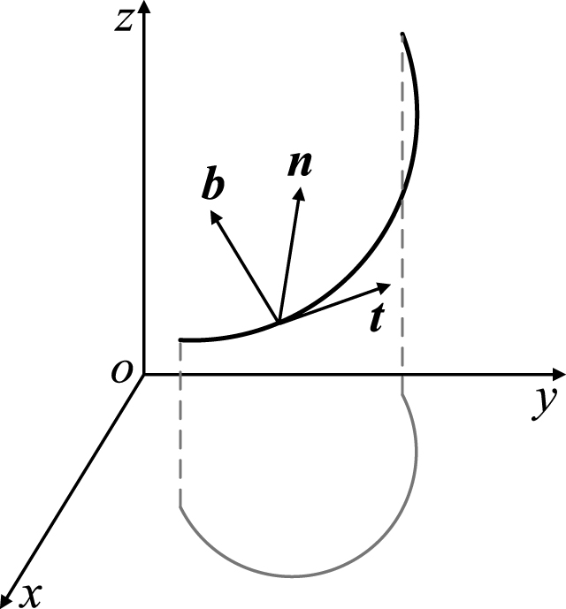
Fig.2
Membership function of variable.
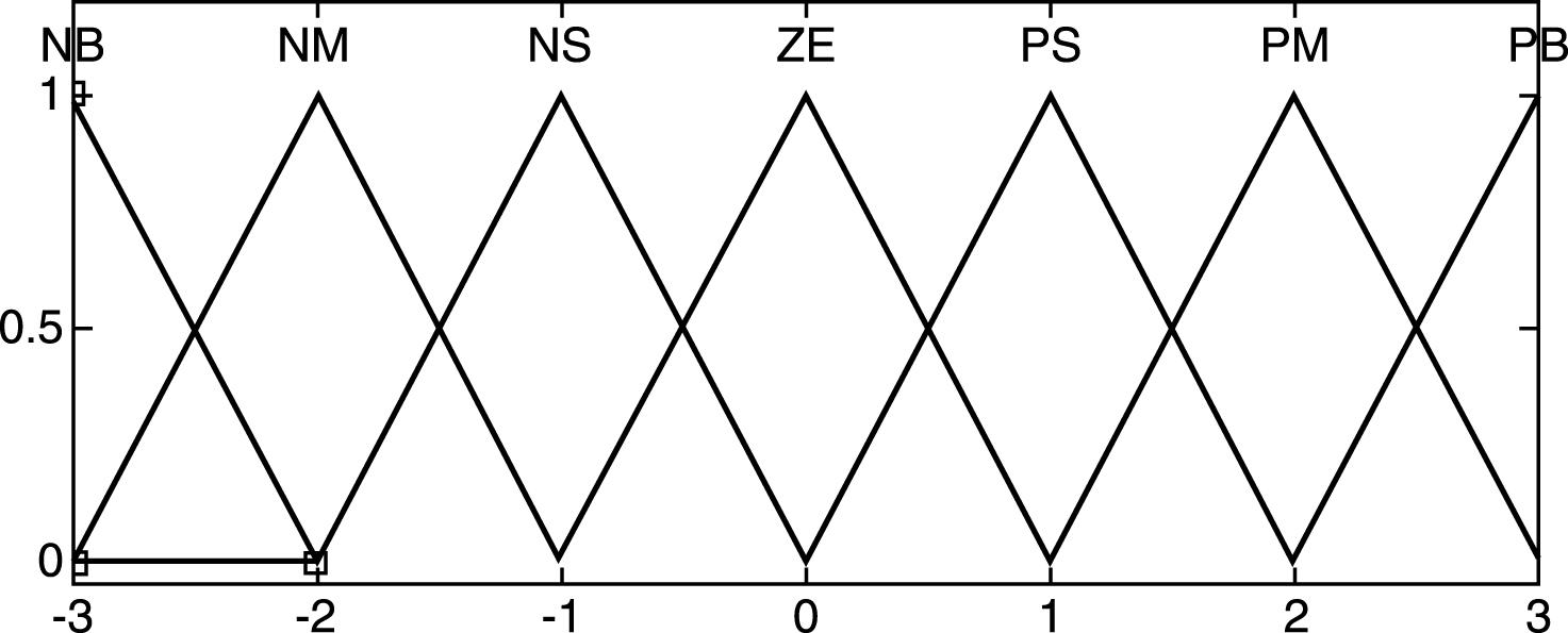
Fig.3
Target acceleration in ys direction.
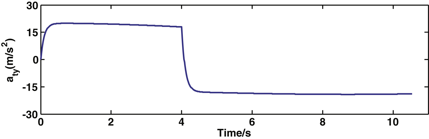
Fig.4
Target acceleration in zs direction.
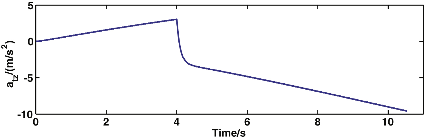
Fig.5
3D trajectories.
Fig.6
Missile acceleration.
Fig.7
Estimation curve of target maneuvering acceleration.
Fig.8
3-D LOS rate curves.
Fig.9
LOS rate in ys direction.
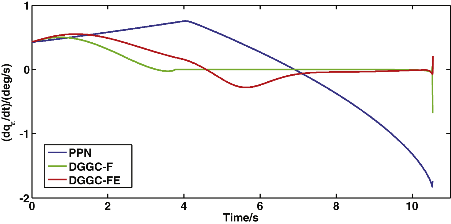
Fig.10
LOS rate in zs direction.
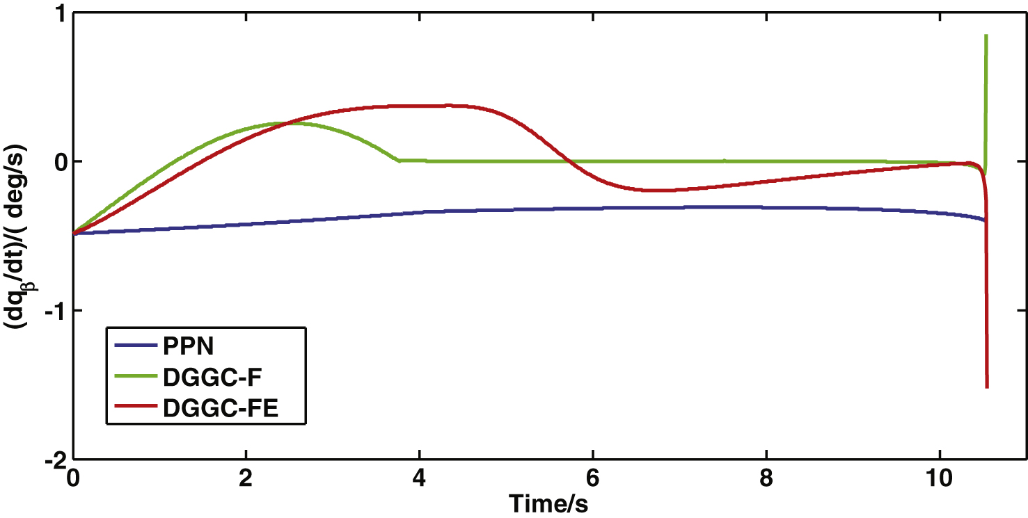
Fig.11
γ curves.
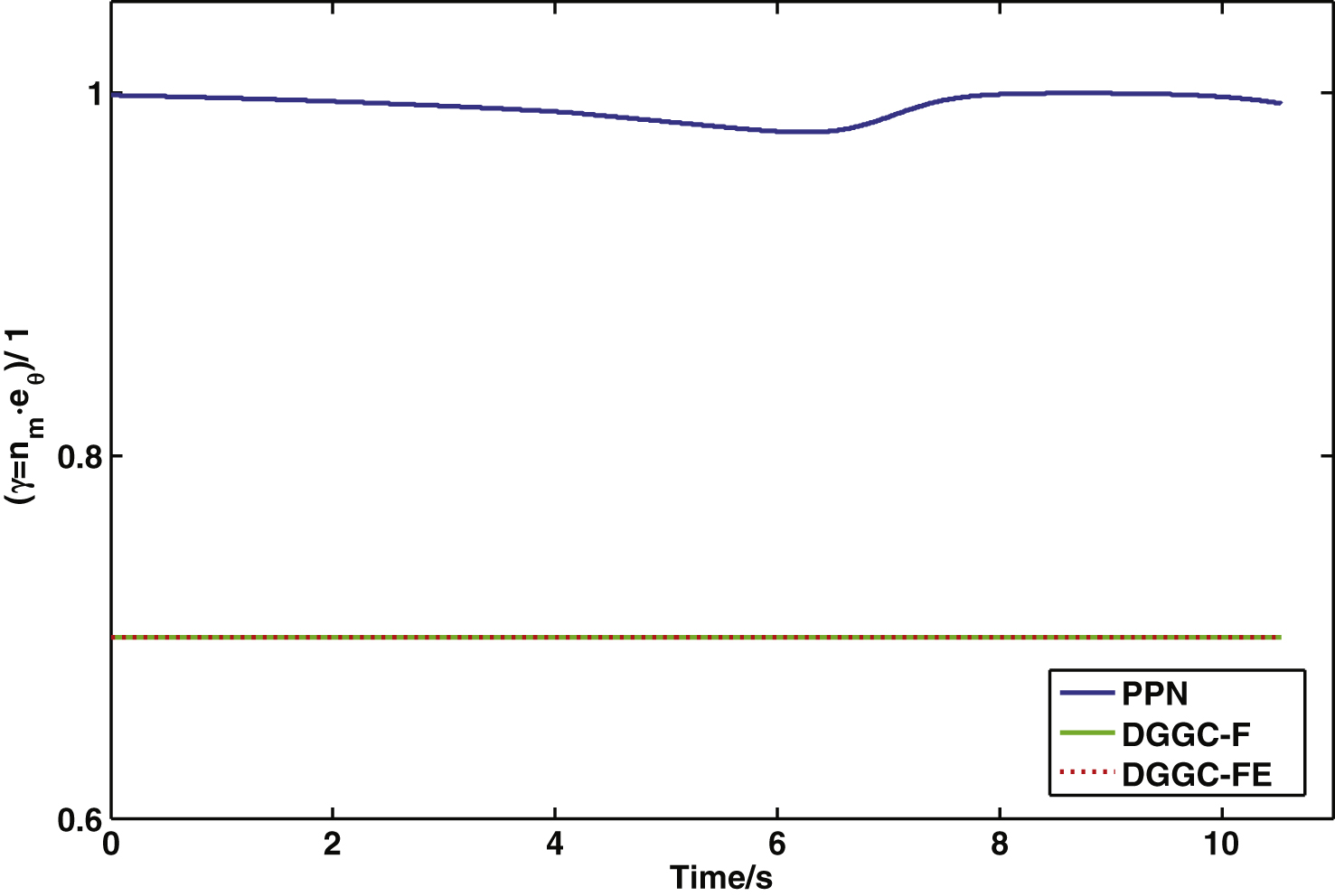
Fig.12
Zero effort miss curves.
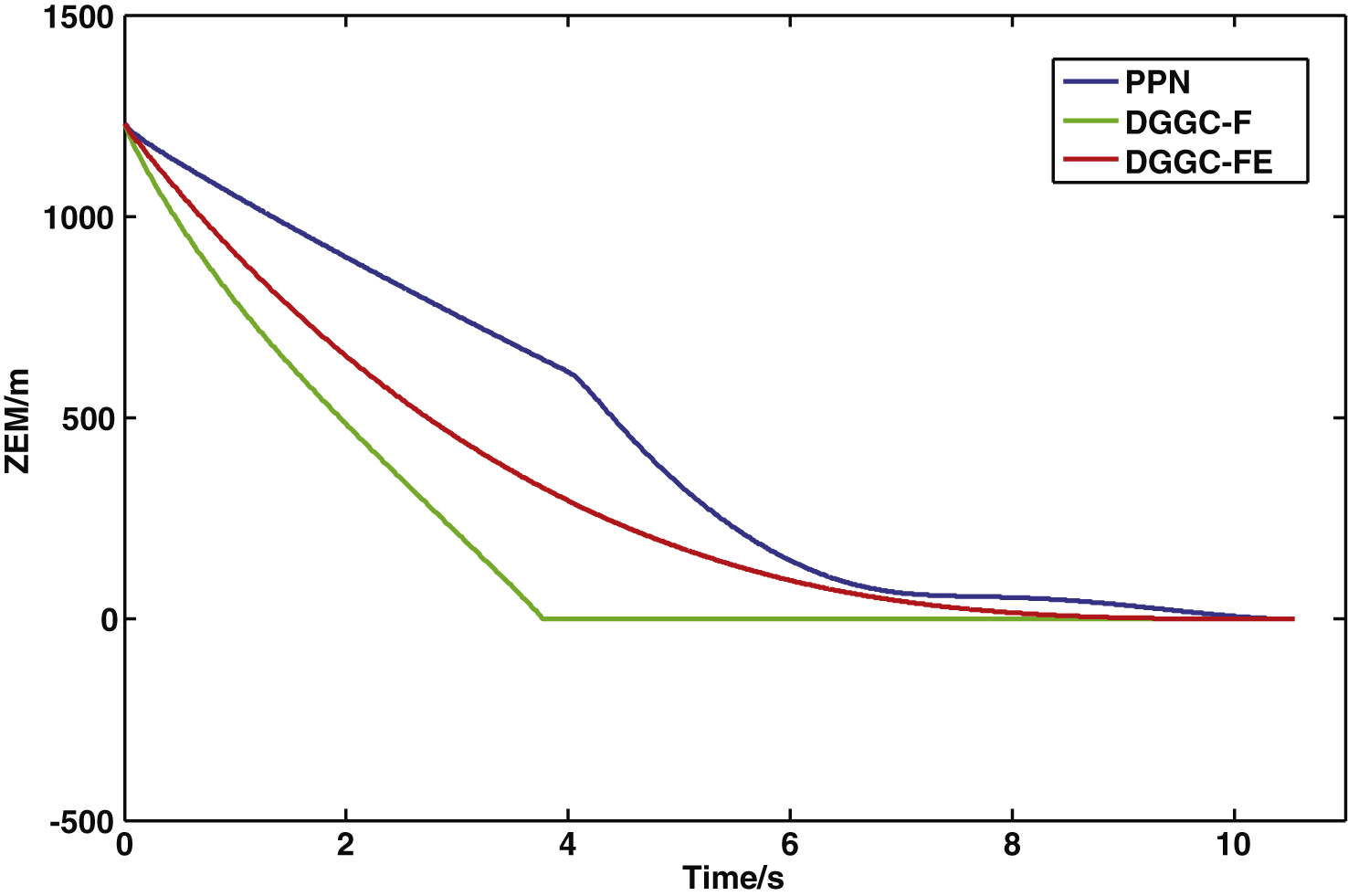
Table 1
Membership functions of linguistic variables
| EC | E | ||||||
| NB | NM | NS | ZE | PS | PM | PB | |
| NB | PB | PB | PM | PM | PS | PS | ZE |
| NM | PB | PM | PM | PS | PS | ZE | NS |
| NS | PM | PM | PS | PS | ZE | NS | NS |
| ZE | PM | PS | PS | ZE | NS | NS | NM |
| PS | PS | PS | ZE | NS | NS | NM | NM |
| PM | PS | ZE | NS | NS | NM | NM | NB |
| PB | ZE | NS | NS | NM | NM | NB | NB |
Table 2
Initial states of missile and target
| Missile | X | Y | Z |
| Position (m) | 0 | 0 | 0 |
| Velocity (m/s) | 629.7667 | 216.0948 | 216.0948 |
| Target | X | Y | Z |
| Position (m) | 10000 | 3000 | 3000 |
| Velocity (m/s) | –400 | 0 | 0 |


