
Interval type-2 fuzzy servo controller for state feedback of nonlinear systems
Abstract
Many researches use T-S fuzzy models to accurately represent nonlinear dynamic systems. However, T-S fuzzy makes the implementation of fuzzy controller more complex as system order and nonlinearities increase. Thus, the present work is aimed to overcome these limitations by using an Interval Type-2 Fuzzy Rule-Based System in which the membership functions and the number of rules can be freely chosen simplifying the implementation of the technique. To this end, it is established a direct state feedback control with reference tracking to generate the nonlinear control action using parallel distributed compensation techniques with no need to include T-S fuzzy models to describe the dynamic system. The proposed strategy is applied to a synchronous generator and also to a magnetic levitation system. From the results, it was verified that IT2FRBSs are able to stabilize the systems analyzed at different equilibrium points with higher performance and less settling times, given the uncertainties in the linearized model. In fact, the IT2FRBS proved to be a proper way to accomplish this task, because fuzzy logic control itself does not depend on an accurate model.
1Introduction
Among the most well-known techniques of Artificial Intelligence is the Fuzzy Logic, introduced in the mid-1960s by L. A. Zadeh [15], whose formulation constituted the starting point for the construction of a structure similar to that used in standard sets, but more general, having greater usability [17] thanks to the concept of a class of elements that admits intermediate degrees of pertinence in a certain set.
For this reason, fuzzy logic allows not only a quantitative but also qualitative analysis of several dynamical systems found in the real world. These systems contain nonlinearities, and were previously considered complex and insufficiently defined to be susceptible to an accurate analysis [19]. For these systems, when the control signals extend beyond the linear operating zones, the system no longer presents approximately linear dynamics [21], and the theory of linear systems was limited only to some special categories.
Furthermore, the state space formulation, when compared to others modeling strategies, is a more powerful alternative model that allows additional advantages, such as: (a) adequate format for the systematization of the solution through computers; (b) state variables constitute a powerful unified structure, suitable for the study of linear and nonlinear systems; (c) allow the development of more robust and efficient methods for digital simulation.
These particularities were determinant to suggest that the fuzzy logic in association with state feedback techniques would be a promising thematic to the study of complex plant control with nonlinear dynamics.
Regarding the uncertainties in the industrial sphere, a solution to define the appropriate adjustment of parameters in relation to a consensus among experts is the use of a formulation, to which the implications of the Takagi-Sugeno method and a fuzzy rule base is used for defining explicit local models [11, 19] known as Takagi-Sugeno fuzzy model (T-Smodels) [23].
Many works have demonstrated that the stability of any dynamic T-S fuzzy system can be determined by verifying an equation of Lyapunov or a set of Linear Matrix Inequalities (LMIs) [1, 26], and others, such as [1, 25, 27, 29] use fuzzy controller based on Parallel Distribution Compensation (PDC) techniques to a proposed T-S model, in which the control problem was transformed into a LMI control design problem.
A disadvantage in using LMI in T-S fuzzy models is that, since if the number of fuzzy IF-THEN rules is large, a common matrix P > 0 maybe does not exists in all the subsystems [1]. So, works sought to suppress the need for the use of LMIs. For example, in [10] the fuzzy control is transformed into a time-varying system by using Riccati Differential Equation.
In the case of nonlinear systems, the control problem for tracking trajectories is occasionally considered relatively difficult in respect to stability problems, since it is expected that the states of the nonlinear system should follow those of the stable model [2, 6].
On the other hand, regarding the nature of uncertainty, in the case of fuzzy systems, any and all kinds of uncertainties is interpreted as being transferred to their membership functions [12]. However, in Fuzzy Rule-Based Systems (FRBSs), the knowledge that is used to construct the rules is also uncertain, and occurs in three ways: (a) the words used in the antecedents and consequences of the rules can have different meanings for different people; (b) the imputation of consequences for a particular rule may be different for different groups of experts; (c) there is accessibility only to a set of noisy data.
It was only later found these deficiencies in traditional fuzzy logic [12] and, in 1975, the concept of type-2 fuzzy was presented by Zadeh as an extension of conventional fuzzy logic (henceforth called type-1 fuzzy logic) [15].
By introducing an additional dimension representing the degrees of membership functions, fuzzy systems could then be formulated as a problem in which membership degrees are themselves fuzzy sets [4].
By eliminating the disadvantages in terms of the modeling of dynamic uncertainties, it was made it possible to develop controllers that use Type-2 fuzzy logic for control, which could be applied to more complex control problems, such as the reference tracking of nonlinear systems for example [8, 13, 28].
In these works, T-S models represent exactly the nonlinear dynamics of the model. However, the use of T-S models increases the implementation complexity of the fuzzy controller by the significant increase of the rule base as system order and nonlinearities increase [10, 24]. To this, researches was conducted to perform the control process, where the type-2 fuzzy model and the type-2 fuzzy controllers do not share the same membership functions [5, 7].
However, in spite of providing greater design flexibility, when the rule bases of the TS model and the controllers are dissociated, the rule base of the model incorporates the rule base of the controller, so that there is an overall increase in the number of rules. Since as the complexity of the model and controller increases, the operation becomes much more difficult, and as consequence, the design procedure of its type-2 fuzzy logic controller tends to be more complicated [21].
Thus, it is suggested a systematic design methodology to design a Fuzzy-Rule-Based System (FRBS) to state feedback with reference tracking of systems with soft nonlinearities in which: (a) does not require T-S fuzzy model representation, requiring only a base of linguistic rules to establish a state feedback control for a class of nonlinear systems found in the real world, (b) the fuzzy controller is able to track a varying reference signal such that drive the system states to the reference (y (t) = r as t→ ∞), (c) allowing the use of techniques previously established in the literature to obtain controllers’ gains, (d) allow easy conversion of Type-1 to an Interval Type-2 FRBS (IT2FRBS).
In the present work, the acronym T1 are used to mention Type-1 fuzzy logic and T2 for Type-2 fuzzy logic. Similarly, IT2 for Interval type-2 fuzzy, and MFs sometimes used to designate Membership Functions.
For validation purposes, the proposed strategy will be applied to two case studies, a magnetic levitation system [9] and a synchronous generator [18, 22].
This paper is organized as follow: Section 2 presents some concepts about a state feedback system with reference tracking. Section 3 introduces the methodological aspects for the development of the proposed IT2FRBS. In section 4 there are some simulation results for which the proposed methodology is adapted to the case studies. In Section 5, the results are analyzed, and finally, some conclusions are presented in section 6.
2State feedback system with reference tracking
Given a fully controllable state system to design a servo controller that guarantees regime error equal to zero, it is necessary to incorporate integrators into the plant before calculating controller gains to integrate the error into the system outputs for which zero-regime error is specified [14].
To avoid the possibility of cancellation of the inserted integrator, it is assumed that the plant does not have zeroes at the origin [3, 14]. Thus, given the linear time-invariant system, the dynamics of the plant with the insertion of the integrators are:
(1)
The controller’s gain matrix is then calculated for the plant with the built-in integrators, so that an asymptotically stable system is designed so that x (∞), v (∞) and u (∞) tend to be constant values, and obtained under a permanent regime y (∞) = r.
Based on these observations, the suggested technique consists, instead of searching for a single point of linearization for the system, of the definition of different balance regions, and thus, the operating space is subdivided into distinct linearization points to obtain local subsystems for the desired balance situations.
The feedback gain matrices can be obtained for each operating point previously established by the designer, using one of the numerous techniques already known in the literature, that is, for each local subsystem whose plant has built-in integrators.
3Proposed fuzzy-rule-based systems (FRBSs)
The T1 Fuzzy-Rule-Based System (T1FRBS) was basically composed of three stages: an input processor, a processing stage composed of a fuzzy rule base and an inference method, and an output stage where the control signal is calculated.
The design methodology for T1FBRS will be explained in more details, since for the construction of the Interval T2FRBS (IT2FRBS), the stages of processing and output obtained are replicated by using the methodology presented for constructing a T1FRBS, and a type-reduction block is added to convert the T2 into T1 fuzzy sets.
3.1Input processor
The input processor is defined by the input variables of the fuzzy controller, where fuzzy variables φ (t) are chosen to be used. Subsequently, the sets of terms of the fuzzy variables are sent to the input processor of the FRBS, and the response at the exit of this stage depends on the MFs corresponding to the terms inserted in the input with the fuzzy input variables.
In this work, the set of dynamic variables φ (t) are suggested as fuzzy variables, so that:
(2)
(3)
In this stage, from the observation of specific criteria, it is possible to optimize the fuzzy system, for which one must consider the supposed knowledge about the circumstances that delimit the system to be controlled to be suitable for practical applications.
Also, a decrease in the number of fuzzy variables decreases the rule base. In this sense, by means of the appropriate choice of a set of state variables, it is possible to choose the output equal to one of the state variables [14]. Based on these aspects, the state variables, which alone do not correspond to the output of interest y (t), are established by definition 1, according to their universes of discourse, such that their MFs corresponds to a constant.
Definition 1. Being U a non-empty set. A subset X ⊂ U is characterized by a membership function μX (x) : U → 1, in which μX (x) is interpreted as being equal to 1 for every value of x belonging to X.
Thus, a set X can be defined by its indicator function, such that given a set X in the universe of discourse U, μX (x) is described by Equation (4).
(4)
In cases where the fuzzy variables are sent to the input system in the form of simple numerical values, intended to obtain the same results in the form of output, the term fuzzy has no explicit distinction, and its MF is represented as a function of constant pertinence.
The fuzzy variables defined in the input processor as constant functions are: state variables x (t) which do not constitute outlets of interest of the system, as well as the vector v (t) from the inserted integrators.
On the other hand, the fuzzy y (t) and
Observation 1. In some cases, for example in the case of MIMO systems that have a high degree of coupling between the outputs, it is also possible to use constant MFs for y (t) and/or
Definition 2. Being U a non-empty set. A subset X ⊂ U is characterized by the membership function μX (x) : U → [0, 1], such that μX (x) is interpreted as the degree to which x belongs to X.
3.2Inference stage and Rule base
The rule base is made up of sentences of the type IF… THEN…, interconnected by connectors of the type AND. Each rule is mathematically translated based on the chosen inference method, and in this work it is used a t-norm to model the AND connective, generating an output for each rule based on definition 3.
Definition 3. Being X1 and X2 fuzzy subsets of U1 and U2, respectively. The membership function of the intersection of X1 and X2 is defined by Equation (5).
(5)
In other words, in the inference stage the relation between the fuzzy sets expressed in their respective universes of discourse is made. Eventually, more than two universes may be related, such that:
Being U1, U2, …, Un universes of the discourse of each fuzzy variable. A fuzzy relation R in U1 × U2 × … × Un is stipulated by the combination:
(6)
Suppose that U1, U2, …, Un are distinct universes of discourse, such that each universe of discourse has a limited number p1, p2, …, pn of MF in U1, U2, …, Un, respectively. μR1 is the grade of membership from the relationship R1 over U1, U2, …, Un, μR2 the grade of membership from relation R2 over U1, U2, …, Un, and being μRw a ω-th grade of membership from relation Rw over U1, U2, …, Un, the composition of these grades of pertinence leads to the construction of a vector of pertinence
(7)
Notably,
Definition 4. Being X a fuzzy subset of U, the support of X, denoted by supp(X), is the subset of U whose elements have non-zero grades of membership in X:
(8)
In order to facilitate the assignment of local controllers, the Equation (3) was used in association with the limits established by the MF of the fuzzy variables corresponding to yp (t) and
Since these variables have their universes of discourses subdivided into MFs, a matrix was created by taking the combination between the lower and upper limits of these MF and the respective reference values that define each situation.
So, for each rule, a critical point matrix called mL is assembled, such that, to the j-th rule:
(9)
Then, a med (mLj) value is defined for mLj, in order to determine the most likely measure of reference to emerge upon activation of this rule, and thus assign the controller that is probably more suitable for a given situation. The value med (mLj) corresponds to the arithmetic mean of the elements of the matrix mLj.
3.3Output processor
The output processor is responsible for calculating the fuzzy control signal uF (t). In this stage, first, it is computed a vector
Thus, it is defined relations such that, Z1 is the control contribution to rule 1 over U1, U2, …, Un, Z2 the control contribution to rule 2 over U1, U2, …, Un, and Zw is the control contribution to the w -th rule over U1, U2, …, Un.
The idea is to assign a compensator K (α) calculated for each of the α balance situations defined in the modeling phase of the system.
In addition to the stability requirements, during the calculation of each compensator K (α), the dynamic behavior desired for the systems at each operating point must also be taken into account, in order to improve transient response and steady state, still in the design phase, so that:
(10)
Each control contribution Z consists of the linear combination of the fuzzy inputs at time, such that for the j-th rule:
(11)
The superscript j indicates the index corresponding to the j-th portion of control contribution calculated for the j-th rule. Therefore, it was defined that: K (α) j indicates the compensator computed for the α-th equilibrium region assigned to the j-th fuzzy rule, as well as Zj(t) is the calculated control contribution for the j-th rule. Zj (t) is initially defined with the help of the matrix mLj proposed in subsection 3.2, which the K (α) j compensator can subsequently be manually adjusted to obtain a more suitable performance for a given situation.
Thus, Zj(t) is given by the linear combination of the fuzzy variables φ (t) according to Equation (12):
(12)
After finalizing the vector
The method used to calculate uF (t) consists of the Takagi-Sugeno fuzzy association between
(13)
Thus, the amount of global fuzzy control signal to be supplied at time t is given by summing the product of each linear control contribution by its respective grades of membership and dividing the result by the sum of all membership.
3.4Interval type-2 fuzzy-rule-based system
In case of the IT2FRBS, the difference is linked to the nature of the MF and not to the rules. Such uncertainties may be related not only to the grades of membership for a particular fuzzy variable φ (t) given its respective fuzzy set, but also in situations where there is uncertainty about the format of the MF or uncertainty in some of its parameters.
To that end, the MF of T2 fuzzy sets include a Footprint Of Uncertainty (FOU) represented by a third dimension capable of providing additional degrees of freedom that make it possible to directly model and deal with the uncertainties of the designer about the meanings of fuzzy associations to be used.
After their definition, the T2 fuzzy sets are moved to the type reduction block, which provides the conversion of the output T2 fuzzy sets, from the Takagi-Sugeno fuzzy association of the local control contributions in
To reduce the computational complexity, it was used interval type-2 fuzzy logic, such that, the type-reducer combines all the output T2 sets by finding their union.
The resulted signal, which follows type-reduction, is based on using the average of outputs
(14)
4Simulation results
For validation purposes, simulations were used to test the proposed methodology, and the results are compared to those obtained using standard state feedback control.
The proposed methodology was applied in two case studies. In the first case study the control of the position of a steel ball in an electromagnetic suspension system [9] is made, and for the second case study the control of the magnetic flux and the load angle in a connected synchronous machine feeding into an infinite busbar [18, 21].
4.1Case study 1: Magnetic levitation system (MAGLEV)
The MAGLEV plant, whose schematic represents in Fig. 1, basically consists of an electromagnet located at the upper part of the apparatus.
Fig.1
Schematic of the MAGLEV plant.
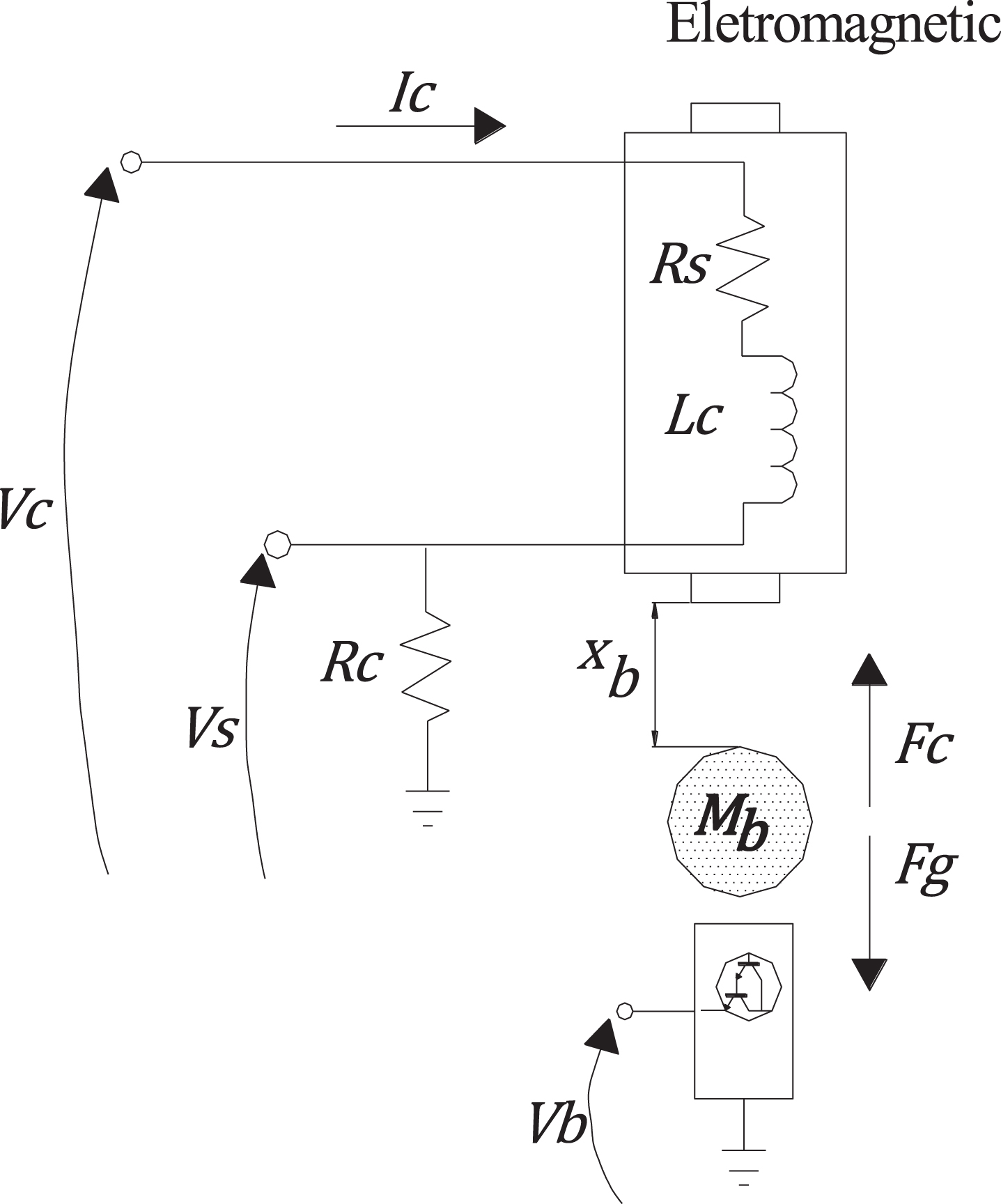
The challenge is to levitate a solid steel ball in the air from the pedestal using an electromagnet, in which only the x-axis is controlled. The control system should maintain the ball stabilized in mid-air and track the ball position to a desired trajectory.
Two variables are directly measured on the MAGLEV rig: The coil current ic (t) and the ball distance xb (t) from the electromagnet face [9].
The coil current can then be computed using Kirchhoff’s voltage law given by Equation (15).
(15)
Fc is the attractive force generated by the electromagnet acting on the steel ball and Fg is the force due to gravity acting on the ball, so that the total external force experienced by the ball using the electromagnet is:
(16)
Using Newton’s second law of motion to the ball gives the nonlinear Equation (17).
(17)
4.1.2Linear space state model
Static equilibrium at a nominal operating point (xb0, ico) is characterized by being suspended in the air at a constant position xb0 due to a constant electromagnetic force generated by ico. The Equation (17) should be linearized around a quiescent operating point (xb0, ico), when it becomes:
(18)
As the objective is to control the position of the ball, the system output of interest is y (t) = xb (t).
The static equilibrium current ico is a function of the system’s desired equilibrium position xb0 and its electromagnet force constant Km.
Different values of ico are evalueteds using different equilibrium positions xb0 and specifications of the MAGLEV [9]. Solving for the equilibrium current:
(19)
Applying the parameters defined in [9] and the intended operating points results in the operating points currents ico to equilibrium positions xb0 in Table 1.
Table 1
Quiescent points (xb0, ic0) used
| Quiescent points (xb0, ic0) | |
| xb0(m) | ic0(A) |
| 0.002 | 0.286 |
| 0.003 | 0.429 |
| 0.004 | 0.572 |
| 0.005 | 0.715 |
| 0.006 | 0.858 |
| 0.007 | 1,001 |
| 0.008 | 1,143 |
| 0.009 | 1,286 |
| 0.010 | 1,429 |
| 0.011 | 1,572 |
| 0.012 | 1,715 |
With the values in Table 1, a local model for each balance situation (xb0, ico) is calculated, and for each local model, a local state feedback controller K (a) is designed using some method disponibilized in literature.
4.2The proposed FRBS adapted to the case study 1
4.2.1Fuzzy input variables
Considering that for the MAGLEV the output y (t) corresponds to one of the state variables (xb (t)), the set of fuzzy variables necessary to control the position of the sphere can be reduced to the set
(20)
and
(21)
Having the fuzzy variables
4.2.2Membership functions
The assignment of the controllers according to the fuzzy rule base essentially requires the values of
Table 2
T1 Membership Functions (T1 MF) from the T1 fuzzy set used to characterize xb (t) e
| xb (t) |
| ||
| T1 Fuzzy set | T1 MF | T1 Fuzzy set | T1 MF |
| xb from 0 to 3 | x2 | Negative maximum error | Nmax |
| xb from 2 to 4 | x3 | Negative Big error | NB |
| xb from 3 to 5 | x4 | Negative Average error | NA |
| xb from 4 to 6 | x5 | Negative Small error | NS |
| xb from 5 to 7 | x6 | Negative minimum error | Nmin |
| xb from 6 to 8 | x7 | Zero error | Z |
| xb from 7 to 9 | x8 | Positive minimum error | Pmin |
| xb from 8 to 10 | x9 | Positive Small error | PS |
| xb from 9 to 11 | x10 | Positive Average error | PA |
| xb from 10 to 12 | x11 | Positive Big error | PB |
| xb from 11 to 14 | x12 | Positive maximum error | Pmax |
4.2.3Rule base
Once the MFs are defined, it is possible to construct the rule base of the FRBS, such that if the output y (t) is xb (t) whose possible values are between zero (without levitation) and 0.014 meters (highest possible height to be reached by the ball). Likewise,
Thus, according to Equation (21), where rxb (t) is known by means of the values of xb (t) and
IF position is “xb” and IF error is “
From the estimate of the desired reference, it is made the assignment is of the most appropriate controller to the quiescent point (α)(xb0, ic0) at time t.
Eleven local controllers K(α) were defined and both variables xb (t) and
As result of each rule, one of the 11 controllers is designed for each of the 11 quiescent points (α)(xb0, ic0).
As the starting point, the assignment of the local controllers do with the help of the measurement med(mLj) from the matrix mLj, presented in subsection 3.2, and from this, fine adjustments are made.
4.2.4Type-2 fuzzy controller
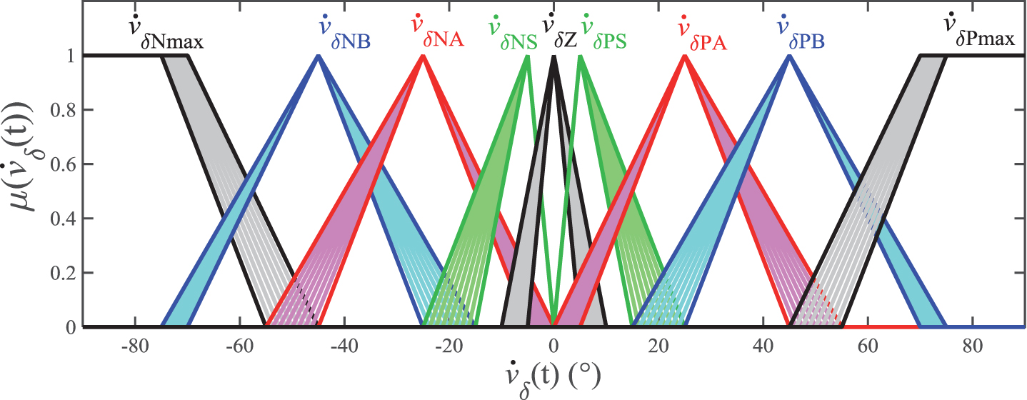
The MFs of the T2 fuzzy sets included a FOU consisting of upper and lower MFs responsible for providing the additional grades of freedom, since the set φ (t) of the input fuzzy variables remains the same.
For the case study 1, the MFs of xb (t) were modified to incorporate an FOU of approximately 0.5 mm in width (Fig. 2). In the case of the MFs that characterize
Fig.2
T2 MFs used to characterize xb (t).
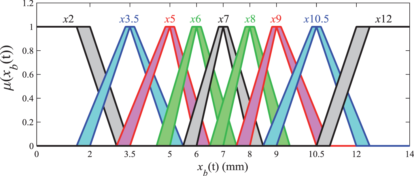
Fig.3
T2 MFs used to characterize
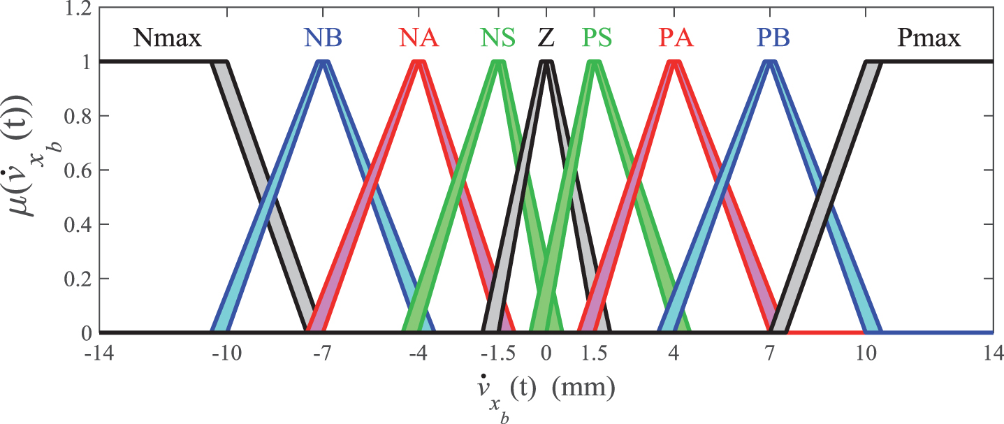
Also, the number of MFs was reduced from 11 to 9 MFs as can be seen in Table 3.
Table 3
T2 MFs from the T2 fuzzy set used to characterize xb (t) e
| xb (t) |
| ||
| T2 Fuzzy set | T2 MF | T2 Fuzzy set | T2 MF |
| xb from 0 to 3.5 | x2 | Negative maximum error | Nmax |
| xb from 2 to 5 | x3.5 | Negative Big error | NB |
| xb from 3.5 to 6 | x5 | Negative Average error | NA |
| xb from 5 to 7 | x6 | Negative Small error | NS |
| xb from 6 to 8 | x7 | Zero error | Z |
| xb from 7 to 9 | x8 | Positive Small error | PS |
| xb from 8 to 10.5 | x9 | Positive Average error | PA |
| xb from 9 to 12 | x10.5 | Positive Big error | PB |
| xb from 10.5 to 14 | x12 | Positive maximum error | Pmax |
4.3Case Study 2: Synchronous machine
In the case study 2, the proposed IT2FRBS is applied to the field flux control, as well as the rotor angle of a synchronous machine feeding into an infinite busbar [18, 21].
4.3.1Nonlinear model
The synchronous machine is represented by a nonlinear model based on the equations of Park [21]:
(22)
For definition:
(23)
The symbology for the variables considered in the model and parameters used, as well as their respective meanings, is presented in the Table 4 [21].
Table 4
List of principals symbols used in case study 2
| Principals symbols | |
| Symbol | Meaning |
| δ | Rotor angle or load angle |
| ω | Rotor speed |
| ψf | Concatenated flux field |
| Efd | Field voltage |
| Tm | Shaft torque input |
| Pg | Governor output |
| V, Vt | Infinite-busbar, generator terminal voltage |
| rf, xf | Field resistance, field reactance |
|
| d-axis armature, d-axis transient reactances |
| xq, xaf, xt | d-axis armature, q-axis mutual, |
| transmission line reactances | |
| H, d | Inertia, damping constants |
| ke | Exciter gain |
| ug, ue | Governor, valve-actuating exciter signals |
| Tt, Tg, Te | Governor, turbine, exciter time constants |
4.3.2Linear space state model
The perturbation in the frequency ω and for the field flux ψf, given in the system of Equation 22, have nonlinear behaviors. Thus, by making the linear approximation around a point of equilibrium (δ0, ψf0), it becomes:
(24)
(25)
The occurrence of some power impact can cause δ (to increase, which can lead to loss of synchronism and, consequently, to instability in the power system [18, 20]. In this sense, δ has a very important role for the stability of the power system. The load angle increases as more electric loads are fed by the generator, and the maximum value for δ is π/2 radians. Above this value, the generator loses synchronism and the stability will be compromised.
So, equilibrium at a nominal operating point (δ0, ψf0) is characterized by being essential for the synchronous machine, and the objective is to keep these variables within a certain margin of safety. For this, different values of ψf0 are evaluated using different values of δ0, with the help of Equation 26 which establishes the voltage Vt at the terminal of the machine [21].
(26)
By applying the parameters defined in Table 5 and the intended operating points results for Vt (t) =1 p.u., the operating points (δ0, ψf0) were obtained and shown in Table 6.
Table 5
Simulation parameters values used in case study 2
| Simulation parameters | |||
| Parameter | Value | Parameter | Value |
| ke | 25 | xt | 0.3 p.u. |
| xd | 1.75 p.u. | xaf | 1.562 p.u. |
|
| 0.2846 p.u. | Tt | 0.3 s |
| H | 3.82 s | Tg | 0.08 s |
| d | 0.006 s | Te | 0.04 s |
| rf | 0.0012 p.u. | V | 1 p.u. |
| xf | 1.665 p.u. | ω0 | 2πfrad/s |
| xq | 1.68 p.u. | f | 60 Hz |
Table 6
Quiescent points (δ0, ψf0) used
| Quiescent points (δ0, ψf0) | |||
| δ0 (°) | ψf0 (p.u) | δ0 (°) | ψf0 (p.u) |
| 0,001 | 1.06731 | 50 | 0.92990 |
| 05 | 1.06547 | 55 | 0.91479 |
| 10 | 1.06000 | 60 | 0.90469 |
| 15 | 1.05105 | 65 | 0.90195 |
| 20 | 1.03889 | 70 | 0.90938 |
| 25 | 1.02390 | 75 | 0.93007 |
| 30 | 1.00657 | 80 | 0.96726 |
| 35 | 0.98758 | 85 | 1.02377 |
| 40 | 0.96773 | 90 | 1.10144 |
| 45 | 0.94808 | ||
With the values in Table 6, a local model for each balance situation is calculated, and for each local model, there is a local state feedback controller K (α).
4.4The proposed FRBS adapted to the case study 2
4.4.1Fuzzy input variables
Considering y1 (t) = δ (t) and y2 (t) = ψf (t)(both state variables), the fuzzy variables suggested to control system is reduced to
(27)
(28)
(29)
4.4.2T2 Membership functions
Having the fuzzy variables
However, in the case of the synchronous machine, there is a high degree of coupling among the output variables, so that when it is intended to control the load angle δ (t), a significant variation is observed in the field flux ψf (t). Likewise, δ (t) it varies as it tries to control ψf (t).
Thus, the frequency-voltage control problem in synchronous machines in interconnected power systems is considered complex, and the frequency, directly influenced by the δ (t), is closely related to the power balance in the entire power grid. Under normal operating conditions the generators operate in synchronism, which represents stable operation, and together they generate the power that is being consumed at all times by all loads.
Considering that the synchronism occurs when δ is constant, because in this situation, the machine enters in steady-state response, the MFs is constructed in such a way that it prevails by the adjustment especially of δ (t). In this case, five MFs were chosen to model the discourse universe of y1 (t) = δ (t), and seven MFs for
Fig.4
T2 MFs used to characterize δ (t).
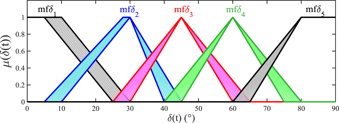
Fig.5
T2 MFs used to characterize
It was found that the control adjustment for small values of δ (t) was more complicated than for averages values of this variable, which suggested that possibly the limits used to delimit the MF responsible for associating δ (t) at small load values should be even smaller. Values above raise0.7exπ / - lower0.7ex4radians presented qualitatively similar responses as δ (t) was increased.
So, the MFs of δ (t) and
The number of MFs remained the same in IT2FRBS because the rule base already contained a sufficient number of rules.
4.4.3Rule base
Possible values to y1 (t) are between zero (without interconnected loads) and raise0.7exπ / - lower0.7ex2radians (maximum load fed by the generator without compromising synchronism). Likewise,
From the estimate of the desired reference rδ (t), the assignment is of the most appropriate controller is made to the quiescent point (α) (δ0, ψ0) at time t, where eighteen local controllers K (α) were defined and both variables δ (t) and
Table 7
T2 MFs from the T2 fuzzy set used to characterize δ (t) e
| δ (t) |
| ||
| T2 Fuzzy Set | T2 MF | T2 Fuzzy Set | T2 MF |
| δ from 0° to 15° | mf δ1 | Negative Big error |
|
| δ from 2° to 25° | mf δ2 | Negative Average error |
|
| δ from 10° to 45° | mf δ3 | Negative Small error |
|
| δ from 25° to 70° | mf δ4 | Zero error |
|
| δ from 45° to 90° | mf δ5 | Positive Small error |
|
| Positive Average error |
| ||
| Positive Big error |
| ||
Thus, a rule base is composed of a total of 45 rules in each output processor block, and the assignment of the local controllers did, initially, with the help of the matrix mLj composed of the association of the limits established by the MFs of δ (t) and
5Analyses and results
The T1FRBS and IT2FRBS were used to control in both case studies and the results compared to those obtained by using standard state feedback.
To compare the performance of T1FRBS, the nonlinear system using standard state feedback was simulated with different K (α) controllers which, unlike the fuzzy controller, maintained their gains static over time, and the control systems were subjected to the same time-varying reference signal r (t) for each case study.
5.1Case study 1
The objective of the control is to make y (t) = xb (t) to follow a continuously changing reference value, in other words, it is desired to maintain the levitating ball in different desired balance positions by means of current adjustments ic (t).
5.1.1T1FRBS versus standard state feedback
In simulations for the case study 1, the r (t) consisted of a set of steps whose amplitudes varied from 0 m to 0.014 m.
The performance obtained by means of the T1FRBS in relation to the standard state feedback control (to static parameters) can be observed in Fig. 6.
Fig.6
Performance of T1FRBS in relation to standard state feedback controller for the case study 1.
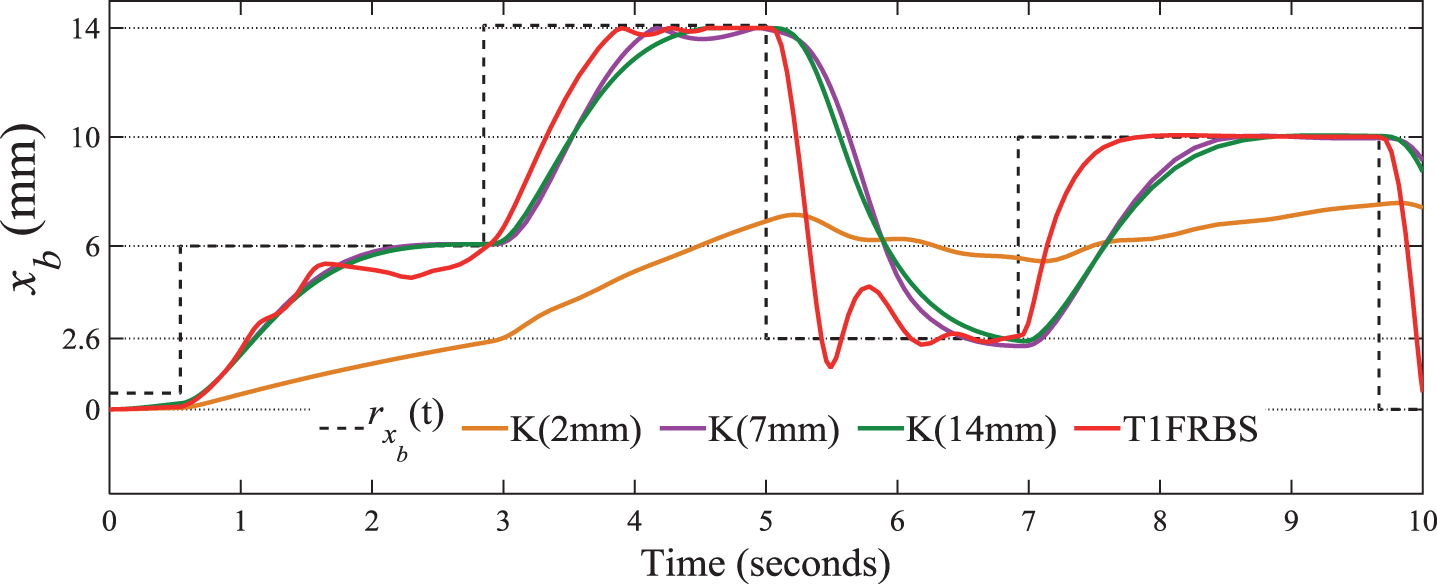
The curves relative to the performances of the controllers with standard state feedback were obtained using controllers calculated to act at different quiescent points corresponding to reference values of 2 mm, 7 mm and 14 mm, respectively.
From the analysis of the curves in Fig. 6, it is observed that the T1FRBS presents superior performance in relation to the control of state feedback to static parameters, since the change in rxb (t) causes a change in the operating point of the dynamic system.
The signal rxb (t) is directly associated with the error
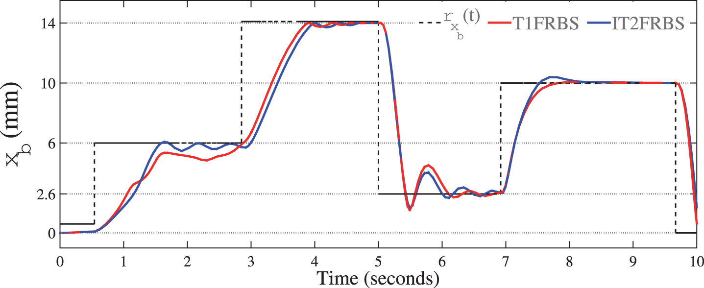
5.1.2IT2FRBS versus T1FRBS
For the composition of the T1FRBS adapted to the case study 1, the universes of the discourse of xb (t) and
Thus, it is convenient to associate some logic capable of handling the uncertainties associated with fuzzy sets, enabling the manipulation of imprecise terms throughout its length. For this, a high amount of MFs is required in order to obtain greater accuracy in the structuring of the fuzzy subsets used.
By inserting T2 fuzzy logic, it was possible to reduce the number of MFs, thus reducing the rule base by about 33%.
Despite the significant reduction of the rules base, it was observed that the performance of the system was similar and, at times, higher than that provided by T1FRBS (Fig. 7).
Fig.7
Performance of T1FRBS in relation to IT2FRBS for the case study 1.
Such superiority is due to the large capacity of T2 fuzzy logic of capturing a combination of values in a set of relevant associations, so that uncertainty can be treated with greater precision in this case, and a single real number is insufficient to provide more information about the uncertainties present. In addition, in order to quantify and satisfactorily model the existing imprecision, measure is needed. In this context, the IT2FRBS conveniently provides this dispersion measure.
5.1.3IT2FRBS using T-S models
For the construction of the T-S model, a very usual method was used [24].
The performance of the control systems for position control in the MAGLEV using the proposed IT2FRBS, in relation to the performance obtained by using the T-S fuzzy model, can be verified in Fig. 8.
Fig.8
Performance of IT2FRBS in relation to T1FRBS using T-S model for the case study 1.
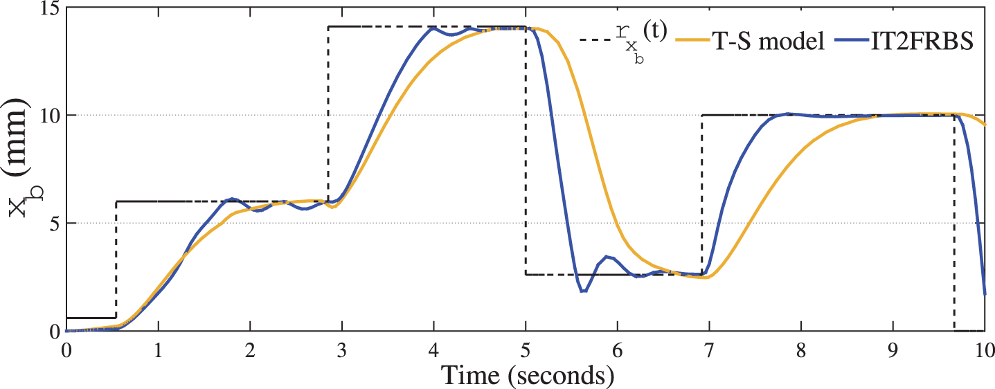
It is verified that the performance using T-S model allowed for a smoother control, while the IT2FRBS, despite showing overshoot in almost all variations of rxb (t), had a faster transient response. Moreover, for the T-S model, all nonlinearities presented are denoted by local models corresponding to the maximum and minimum values of each nonlinear term in the equations of the system. Thus, the number of local models for each operating region is directly related to the number of nonlinear terms present.
Since Equation (17), which governs the behavior of MAGLEV, has two nonlinear terms, four local fuzzy models are required to represent the nonlinear system in such specific operating region, and it is necessary to calculate a new compensator for each fuzzy subsystem. Thus, for the elaboration of the T-S model, by using the number of delimited regions equal to the number of operating points established in the elaboration of FRBSs, the rule base was increased to a total of 1331 rules. This increase in the rule base is explained by the fact that the nonlinear term corresponding to ic (t), which in the methodology proposed in this work could be described by a constant MF, in the T-S modeling is described by a set of triangular and trapezoidal MFs, limited by the regions of operations.
5.2Case study 2
In a Power System, the controller is designed to: (a) In the occurrence of random power-impacts, the added power must be supplied by the synchronous generators, (b) to maintain a scheduled power exchange over the tie-line in the interconnected system.
In this sense, δ has a very important role, because some power-impact, such as abrupt changes in the interconnected load, can make it vary considerably, which can cause loss of synchronism and, consequently, instability in the power system.
Thus, the control objective in this case study is to make the outputs
5.2.1T1FRBS versus standard state feedback
In simulations for the case study 2, the rδ (t) consists of a set of steps whose amplitudes vary from 0 up to
The performance obtained by means of the T1FRBS in relation to the standard state feedback control is observed in Fig. 9.
Fig.9
Performance of T1FRBS to the control of δ (t),in relation to standard state feedback controller for the case study 2.
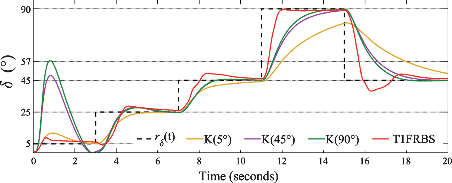
For the simulations with standard state feedback controllers, three controllers (K(5°), K (45°) and K(90°)) were used to operate in three distinct equilibrium regions (δ0, ψf0), in Table 6, where δ0 correspond to 5°, 45° and 90°, respectively.
In Fig. 9, it is verified that the performance obtained using all three standard state feedback controllers allowed for a smoother control of the load angle for higher values of δ, whereas for small values of δ, the controllers with fixed parameters present high overshoot.
Thus, by using only fixed gain control, there would be problems related to the lack of performance using controllers designed for situations of low values of interconnected load, which would complicate the control problem in situations of high load because, in this situation, the high non-linearity present in the system was more difficult to control. In addition, an excessively smooth control system can cause very slow responses to load disturbances.
On the other hand, for situations of low load demand, there would be problems of peaks in the load angle with the use of controllers with a “tight” tuning, designed for situations of high load, which would lead to a fast control action, but with a drastic variation in the frequency amplitude of the power system. In this case, the control action is very fast, and constantly varies by the difference between δ (t) and rδ (t), in order to make the control system more vulnerable to instabilities.
The T1FRBS, despite showing small overshoot in almost all variations of rδ (t), but with a faster transient response, even in situations of low load angle the response presents a smaller overshoot than the one corresponding to the fixed gain controller calculated for this region. The field flux behavior, seen in Fig. 10, shows that the proposed fuzzy system can follow the reference rψf (t), but presents overshoots during the transient period. The effect of this oscillation during the transient period is reflected in the terminal voltage Vt (t), given by Equation 26, of the synchronous generator and can be seenin Fig. 11.
Fig.10
Performance of T1FRBS, to the control of ψf (t), in relation to standard state feedback controller for the case study 2.
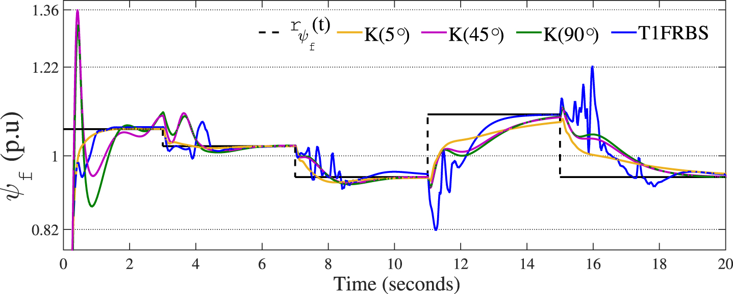
Fig.11
Terminal voltage Vt (using T1FRBS in relation to use standard state feedback controller for the case study 2.
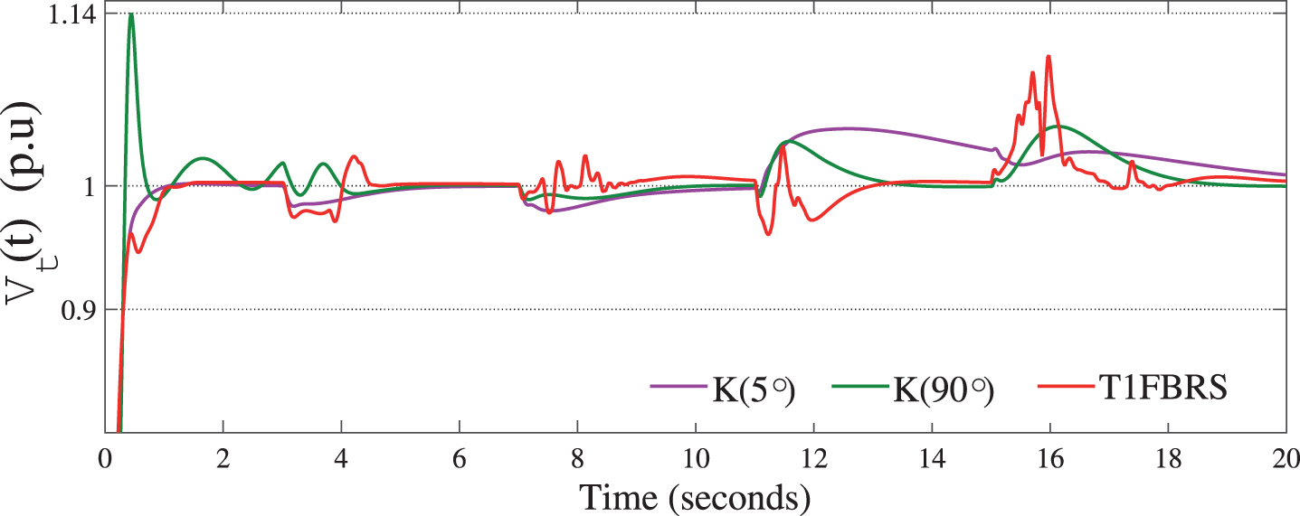
In relation to use standard state feedback controller, whether tight or smooth tuning, the T1FRBS presented satisfactory performance, characterized by faster transient, besides keeping the oscillations within a mean lower limit than that obtained with the use of controllers with fixed parameters.
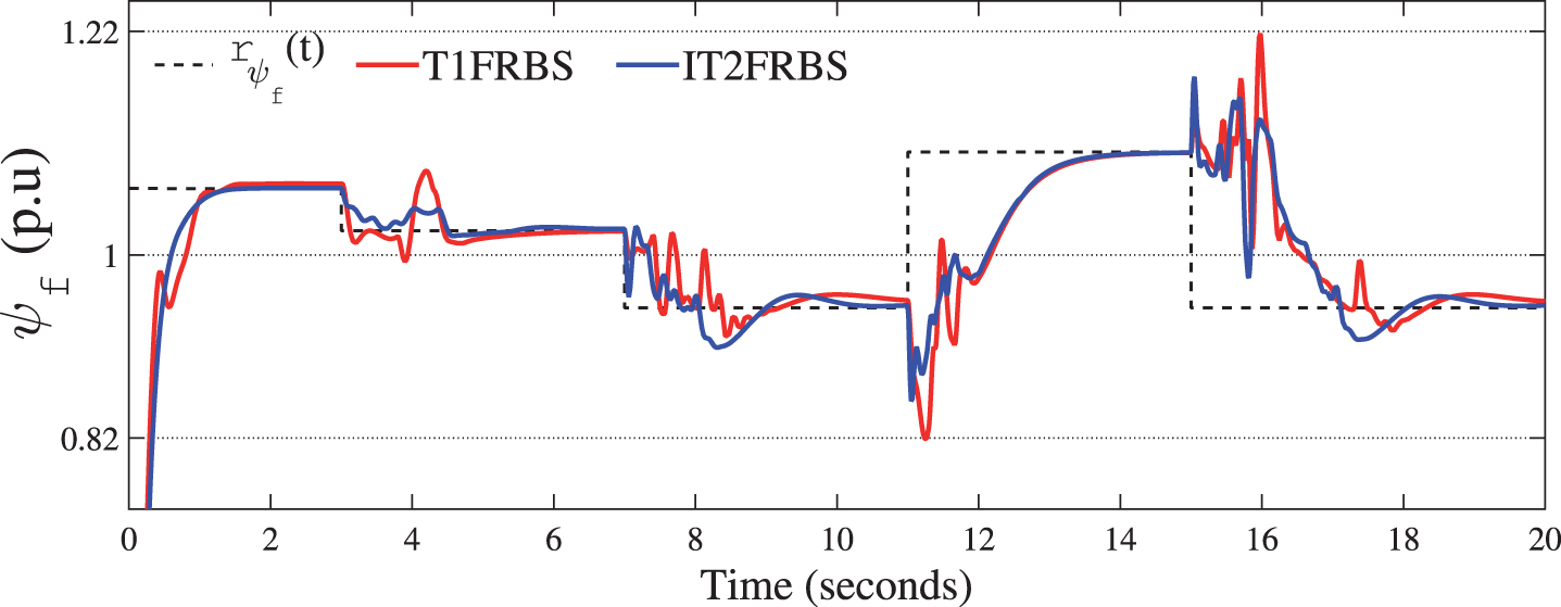
5.2.2IT2FRBS versus T1FRBS
The proposed IT2FRBS was tested for case study 2, and the performance obtained was compared to the good performance obtained by T1FRBS.
For the construction of IT2FRBS, only FOUs were added to the MFs as quoted in subsection 3.4, in other words, only the inference blocks and output processor were duplicated to receive the new set of MFs, in addition to the inclusion of the type-reducer block.
The performances resulting from the use of the proposed IT2FRBS can be seen in Fig. 12 to the control of δ (t).
Fig.12
Performance of T1FRBS, to the control of δ (t), in relation to IT2FRBS for the case study 2.
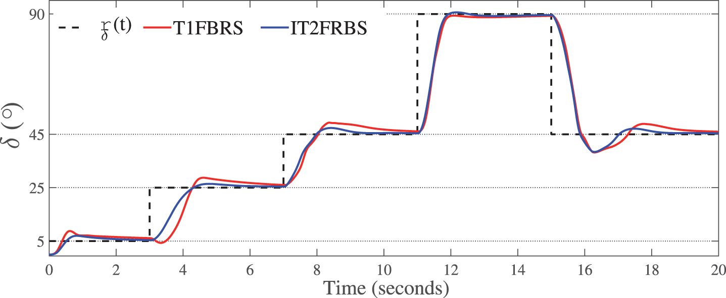
In the case study 2, the IT2FRBS provided a higher performance of the system than that provided by T1FRBS for all load situations tested and sudden loads transitions, both in relation to the transient response, characterized by faster responses and lower overshoots, as well as in relation to steady-state response, with the elimination of the steady-state error.
In addition, it provides control with the advantages of the smoother action than the T1FRBS when necessary, but also inhibits the excess of slowness to the rejection of disturbances in the interconnected load thanks to the insertion of FOUs that made it possible to handle the uncertainties associated with fuzzy sets that characterized δ (t), providing a better treatment of imprecision in its all universe of discourse.
Since there is a high degree of coupling between the variables
Fig.13
Performance of T1FRBS, to the control of ψf (t), in relation to IT2FRBS for the case study 2.
The control of the field flux implies the control of the terminal voltage. Consequently, the advantages provided by the performance of the IT2FRBS in substitution for the T1FRBS are also reflected in the trajectory of Vt (t), which can be verified in Fig. 14.
Fig.14
Terminal voltage Vt (t) using T1FRBS in relation to use IT2FRBS for the case study 2.
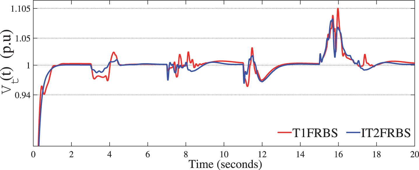
These higher performances of IT2FRBS are due to the fact that T1 fuzzy sets are able to effectively capture the system nonlinearities but not theuncertainties [5].
By choosing simple MFs such as turning the MFs to yψf (t) and
5.3About results
The superior performance achieved by the T1FRBSin relation to the standard state feedback control is due to the fact that a control system that presents linear dynamic behavior with static parameters sometimes becomes unable to provide enough flexibility to attend all the performance specifications, by means of the present variations.
It is also known that conventional control theories, established by rigorous analyzes, cannot satisfactorily deal with the complexity, nonlinearity, and imprecision of many real control systems. In contrast, the rule base of the FRBS allows the allocation of more suitable controllers to different load situations.
By the proposed method, it uses a linguistic rule-based to generate the nonlinear control action from the linear combination of a set φ (t) of pre-defined fuzzy variables, such that the problem of fuzzy control of reference tracking can be solved by making use of control techniques for linear systems. Thus, for each rule, it can use linear control design techniques, but the resulting overall fuzzy controller, which is a fuzzy blending of each individual linear controller, is nonlinear.
The PDC techniques, in association with fuzzy logic, allow the change from one local controller to another to occur gradually, not abruptly, as would happen without the implication of degrees of pertinence attributed to input fuzzy variables, so that depict the nonlinearities present. The MFs responsible for qualifying error allocate tightest local controllers K (α) when the error is large and K (α) controllers less tight while the error decreases.
The situation where the contribution Zj for the vector
In T2 fuzzy, the limit
Thus, some rules that were not activated in a given situation in the upper MFs started to be activated in the lower MFs, as well as in a reciprocal way. Moreover, even in situations where a rule j is activated in both cases, the contributions Zj relative to the consequence of the j-th rule of the vector
For this reason, T2 fuzzy logic allows a gradual transition from nonlinear control modes to upper and lower MFs, and consequently to uncertainty about the limits that best characterize a given situation.
In other words, IT2FRBS can be conveniently used in situations where there is uncertainty about the grades of membership, the uncertainty of the format of MFs and uncertainty in some of the parameters of MFs, such as the limits established for MFs. Thus, thanks to the remarkable ability to handle uncertainties in the control area, controllers that use T2 fuzzy logic have been gaining more and more space in recent years.
Case study 1 proposed IT2FRBS to a fuzzy state feedback control using T-S fuzzy models. Controllers obtained by T-S fuzzy models adapt to different situations within the region of operation for which they were defined. In this case, their global stability is guaranteed when looking to take a system from one point to another within a defined convex region. It does not happen when using local linear models obtained by linearization around an operating point so that the system is not guaranteed to be stable when it is moving through points within the specified region. However, even using T-S models, it is required to ensure stability that the IT2 fuzzy controller shares the same premise MFs and the same number of rules as those of the IT2 T-S fuzzy model [5].
When it uses T-S models, however, the number of local models increases with the nonlinearities. These limitations constrain not only the design flexibility of the controllers, but also increase the implementation complexity of the IT2 fuzzy controller by the significant increase of the rule base.
On the other hand, since T-S model is not necessarily implemented [7], a direct IT2FRBS allows the number of MFs used to be freely chosen and, as a consequence, there is more autonomy on the part of the control designer, which would be responsible for balancing between more accuracy of response and computational complexity.
6Conclusions
This work proposed systematic procedure to design a control strategy that uses an IT2FRBS for state feedback and reference tracking of nonlinear systems.
Two case studies were analyzed with the application of the proposed systematics. The performance of the proposed FRBS was analyzed using T1 in relation of T2 logic and it was found that IT2FRBS perform better in relation to T1FRBS for transient and steady-state responses, even with a smaller amount of MFs (in the case study 1), and consequently, fewer rules.
The proposed IT2FRBS was also compared with a T1FRBS using T-S models to the case study 1, where it was found that the IT2FRBS was able to not only stabilize the system, but also to do so with less settling time and using a much lower rule base.
The methodology proposed overcomes some of the limitations related to the project design for several complex systems by proposing an IT2FRBS since, by a direct control, only local linear controllers are used without the need to include T-S fuzzy models on the rule-base nor complicated adaptive schemes. In this case the MFs and the number of rules can be freely chosen, enhancing the applicability by providing increases the ease of implementation of the technique.
From the results, it was verified that T1FRBSs is able to stabilize the systems analyzed at different equilibrium points, but the performance of the IT2FRBS is much smoother and it needs less settling times, and given the quantity of uncertainties in the linearized model. In fact, the IT2FRBS proved to be a proper way to accomplish this task, because fuzzy logic control itself does not depend on an accurate model of the controlled object, and the IT2 MFs of the fuzzy control are able to handle parameter uncertainties arising from the linearization.
The achievement of the results made it possible to establish sufficient and necessary conditions for the implementation of the proposed strategy to solve the lack of a generic procedure to a systematic form of calculation definite during utilization of fuzzy sets, which provide the basis of the elaboration of efficient servo controllers, applicable to several situations, despite the presence of some kind of nonlinearities and source of uncertainties.
Future work should investigate the performance of this methodology by extending the results from the approximations of Generalized T2 fuzzy systems based on several IT2 fuzzy systems by the concept of α-planes representation.
Acknowledgment
The authors thank to the Post-Graduation Program in Electrical and Computer Engineering of the Federal University of Rio Grande do Norte - PPGEEC / UFRN - for the technical and administrative support, and to the Coordination of Improvement of Higher Education Personnel - Ministry of Education (Capes - MEC) for granting research scholarship to the corresponding author.
References
[1] | C. Feng and L. Chang , Robust Takagi-Sugeno fuzzy control for nonlinear singular time-delay hydraulic turbine governing system, International Symposium on Computational Intelligence and Design (ISCID) ((2018) ). |
[2] | C.-S. Tseng , B.-S. Chen and H.-J. Uang , Fuzzy tracking control design for nonlinear dynamic systems via T–S fuzzy model, IEEE Transactions on Fuzzy Systems 9: ((2001) ). |
[3] | C.-T. Chen , Linear System Theory and Design, 3th edition, Oxford University Press, New York, (1999) . |
[4] | D. Wu And and J.M. Mendel , Similarity measures for closed general type-2 fuzzy sets: Overview, Comparisons, and a Geometric Approach, IEEE Transactions On Fuzzy Systems 27: ((2019) ), 515–526. |
[5] | H.K. Lam , H. LI , C. Deters , H.A. Wuerdemann , E.L. Secco and K. Althoefer , Control design for interval type-2 fuzzy systems under imperfect premise matching, IEEE Trans on Industrial Electronics 61: ((2014) ), 956–968. |
[6] | H.K. Lam and L.D. Seneviratne , Tracking control of sampled-data fuzzy-model-based control systems, IET Control Theory and Applications 3: ((2009) ), 56–67. |
[7] | H. Li , X. Sun , L. Wu and H.K. Lam , State and output feedback control of interval type-2 fuzzy systems with mismatched membership functions, IEEE Transactions on Fuzzy Systems 23: ((2015) ), 1943–1957. |
[8] | H.-S. Chen and W.-S. yu , Interval Type-2 Fuzzy Model Based Indirect Adaptive Tracking Control Design for Nonlinear Systems With Dead-Zones, IEEE International Conference on Fuzzy Systems, (2010) , pp. 1–6. |
[9] | J. Apkarian , H. Lacheray and M. Lévis , Magnetic Levitation Experiment for MATLAB /Simulink Users: Instructor Workbook, Quanser Inc., (2012) . |
[10] | J. Cervantes , W. Yu and S. Salazar , On-line T-S fuzzy control using Riccati differential equation, Journal of Intelligent & Fuzzy Systems 33: ((2017) ), 3871–3881. |
[11] | J. Li , J. Wang and M. Chen , Modeling and control of Takagi-Sugeno fuzzy hyperbolic model for a class of nonlinear systems, Journal of Intelligent & Fuzzy Systems 33: ((2017) ), 3265–3273. |
[12] | J.M. Mendel , Type-2 fuzzy sets: Some questions and answers, IEEE Neural Network Society 1: (2003) ((2015) ), 10–13. |
[13] | K.B. Meziane and I. Boumhidi , An Interval Type-2 Fuzzy Logic PSS with the optimal H∞ tracking control for multi-machine power system, Intelligent Systems and Computer Vision, 1–8. |
[14] | K. Ogata , Engenharia de Controle Moderno, 5th edition, Pearson Prentice Hall, (2010) . |
[15] | L.A. Zadeh , Fuzzy sets, Information And Control l8: ((1965) ), 338–353. |
[16] | L.A. Zadeh , The concept of a linguistic variable and its application to approximate reasoning-I, Information Sciences 8: ((1975) ), 199–249. |
[17] | L.A. Zadeh , Interview with lotfi zadeh, creator of fuzzy logic, azerbaijan internetional, Interview with Betty Balir 50: ((1994) ), 46–47. |
[18] | M.V.A. Fernandes , A.D. Lima and A.D. Araújo , Variable Structure Model Reference Adaptive Controller Applied to a Synchronous Generator Control, Mediterranean Conference on Control and Automation Congress Centre, (2008) . |
[19] | N. Manamanni , B. Mansouri , A. Hamzaoui and J. Zaytoon , Relaxed conditions in tracking control design for a TS fuzzy model, Journal of Intelligent & Fuzzy Systems 18: ((2007) ), 185–210. |
[20] | P. Kundur , Power System Stability and Control, 1th edition, McGraw-Hill Professional Publishing, (1994) . |
[21] | S. Ding , X. Huang , X. Ban , H. Lu and H. Zhang , Type-2 fuzzy logic control for underactuated truss-like robotic finger with comparison of a type-1 case1, Journal of Intelligent & Fuzzy Systems 33: ((2017) ), 2047–2057. |
[22] | S.N. Singh , Nonlinear state-variable-feedback excitation- and governor-control design using decoupling theory, IEEE Proceedings 12: ((1980) ). |
[23] | T. Takagi and M. Sugeno , Fuzzy identification of systems and its applications to modeling and control, IEEE Transaction on Systems, Man and Cybernetics SMC 15: ((1985) ), 116–132. |
[24] | T. Taniguchi , K. Tanaka , H. Ohtake and H.O. Wang , Model construction, rule reduction, and robust compensation for generalized form of takagi–sugeno fuzzy systems, IEEE Transactions on Fuzzy Systems 9: ((2001) ), 525–538. |
[25] | Y.-G. Sun , J.-Q. Xu , C. Chen and G.-B. Lin , Fuzzy H∞ robust control for magnetic levitation system of maglev vehicles based on T-S fuzzy model: Design and experiments, Journal of Intelligent & Fuzzy System. DOI: 10.3233/JIFS-169868 |
[26] | Y.-T. Juang , C.-L. Yan and C.-P. Huang , Relaxed stability issues for T-S fuzzy system: Based on a fuzzy quadratic Lyapunov function, Journal of Intelligent & Fuzzy Systems 26: ((2014) ), 667–679. |
[27] | Z. Du , Y. Kao and J.H. Park , Interval type-2 fuzzy sampled-data control of time-delay systems, Information Sciences 487: ((2019) ), 193–207. |
[28] | Z. Du , Z. Yan and Z. Zhao , Interval type-2 fuzzy tracking control for nonlinear systems via sampled-data controller, Fuzzy Sets and Systems 356: ((2019) ), 92–112. |
[29] | Z. Zhang , H. Liang , C. Wu and C.K. Ahn , Adaptive event-triggered output feedback fuzzy control for nonlinear networked systems with packet dropouts and actuator failure, IEEE Transactions on Fuzzy Systems ((2019) ). |


